Bayesian versus frequentist upper limits

Abstract

While gravitational waves have not yet been measured directly, data analysis from detection experiments commonly includes an upper limit statement. Such upper limits may be derived via a frequentist or Bayesian approach; the theoretical implications are very different, and on the technical side, one notable difference is that one case requires maximization of the likelihood function over parameter space, while the other requires integration. Using a simple example (detection of a sinusoidal signal in white Gaussian noise), we investigate the differences in performance and interpretation, and the effect of the “trials factor”, or “look-elsewhere effect”.

1 Introduction

1.1 Upper limits

In general, an upper limit is a probabilistic statement bounding one of several unknown parameters determining the observed data at hand. While it would be hard to derive general properties applicable in any possible data analysis context, we will for the illustration purpose consider a simple case here: a sinusoidal signal in white Gaussian noise. This example exhibits many similarities with commonly encountered real-world problems, including the use of Fourier methods, nuisance parameters, trials factors, partly analytical and numerical analysis, etc., and we believe is general enough to yield valuable insights.

1.2 The frequentist case

The frequentist detection approach is based on some detection statistic $d$, which for given data is then used to derive a significance statement along the lines of “If the data were only noise (null hypothesis $H_{0}$), a detection statistic value $\geq d_{0}$ would have been observed with probability $p$.” ($\mathrm{P}(d\geq d_{0}\,|\,H_{0})=p$). The probability $p$ here is the p-value, and a low p-value is associated with a great significance. In the case of a non-detection, the statement then may be reversed to an upper limit statement “Had the signal amplitude been $\geq A^{\star}$, a larger detection statistic value ($\geq d_{0}$) would have been observed with at least 90% probability” ($\mathrm{P}(d\geq d_{0}\,|\,A\geq A^{\star})\geq 90\%$), where $A^{\star}$ is the 90% confidence upper limit (e.g. [1, 2]).

1.3 The Bayesian case

In the Bayesian framework, detection and parameter estimation are more separate problems; for detection purposes one would need to derive the marginal likelihood, or Bayes factor, which (in conjunction with the prior probabilities for the “signal” and “noise only” hypotheses $H_{1}$ and $H_{0}$) allows one to derive the probability for the presence of a signal. The detection statement would then be “(Given the observed data $y$,) the probability for the presence of a signal is $p$.” ($\mathrm{P}(H_{1}|y)=p$). The upper limit statement on the other hand is a matter of parameter estimation; given the joint posterior distribution of all unknowns in the model, one would need to marginalize to get the posterior distribution of the parameter of interest alone. The upper limit statement would then be “(Given the observed data and the presence of a signal,) the amplitude is $\leq A^{\star}$ with 90% probability.” ($\mathrm{P}(A\leq A^{\star}\,|\,y,H_{1})=90\%$) [3, 4].

2 The data model

We assume the data $y$ to be a time series given by a parameterized signal $s$ and additive noise $n$:

$$y(t_{i})\;=\;s(t_{i})+n(t_{i}),$$ (1)

where $i=1,\ldots,N$ and $t_{i}=i\Delta_{t}$. The (sinusoidal) signal is given by

$$s(t)\;=\;A\,\sin(2\pi ft+\phi),$$ (2)

where $A\geq 0$ is the amplitude, $0\leq\phi<2\pi$ is the phase, and $f\in\{\frac{j_{1}}{N\Delta_{t}},\ldots,\frac{j_{k}}{N\Delta_{t}}\}$ is the frequency, where $1\leq j_{1},\ldots,j_{k}\leq\frac{N}{2}-1$ defines the range of possible (Fourier) frequencies. The number $k$ of frequency bins may be varied and constitutes the so-called “trials factor” here. The noise $n$ is assumed to be white and Gaussian with variance $\sigma^{2}$.

3 Frequentist approach

If there were no unknown parameters in the signal model, then, following from the Neyman-Pearson lemma, the optimal detection statistic would be given by the likelihood ratio of the two hypotheses. In the case that the hypotheses include unknowns (composite hypotheses) as in our case, this is commonly treated using the generalized likelihood ratio framework, that is, by considering the ratio of maximized likelihoods, where maximization is done over the unknown parameters [5].

In our case, we have a 3-dimensional parameter space under the signal model. The conditional likelihood for a given frequency may be maximized analytically over phase and amplitude. The profile likelihood (maximized conditional likelihood for given frequency, as a function of frequency) is eventually proportional to the time series’ periodogram. The generalized likelihood ratio detection statistic then is given as the periodogram maximized over the frequency range of interest:

$$d^{2}\;:=\;\max_{j}\,{\textstyle\frac{2}{N\sigma^{2}}}\big{|}\tilde{y}_{j}\big{|}^{2}$$ (3)

where $\tilde{y}_{j}$ is the (complex valued) $j$th element of the discretely Fourier transformed time series $y$. The “$\frac{2}{N\sigma^{2}}\big{|}\tilde{y}_{j}\big{|}^{2}$” term (the periodogram) maximized over in (3) is in fact also the matched filter for a sinusoidal signal [6], and the maximum $d^{2}$ is commonly referred to as the “loudest event” [2].

The detection statistic’s distribution may be derived analytically under both hypotheses $H_{0}$ and $H_{1}$, as this is a particular case of an extreme value statistic [5]. Under the null hypothesis, $d^{2}$ is the maximum of $k$ independently $\chi_{2}^{2}$-distributed random variables; the cumulative distribution function (CDF) of $d^{2}$ is given by

$$F_{d^{2};H_{0}}(x)\;=\;\mathrm{P}(d^{2}\leq x\,|\,H_{0})\;=\;\bigl{(}F_{\chi_{2}^{2}}(x)\bigr{)}^{k}$$ (4)

where $F_{\chi_{2}^{2}}$ is the CDF of a $\chi_{2}^{2}$ distribution, and $k$ again is the number of independent frequency bins, or “trials”. This is essentially the “background distribution” of $d^{2}$. Under the signal hypothesis $H_{1}$, $d^{2}$ is the maximum of $(k\!-\!1)$ independently $\chi_{2}^{2}$-distributed random variables and one noncentral-$\chi_{2}^{2}(\lambda)$-distributed variable with noncentrality parameter $\lambda=\frac{N}{2\sigma^{2}}A^{2}$. The corresponding CDF under $H_{1}$ then is

$$F_{d^{2};H_{1}}(x)\;=\;\bigl{(}F_{\chi_{2}^{2}}(x)\bigr{)}^{(k-1)}\times F_{\chi_{2,\lambda}^{2}}(x)$$ (5)

where $F_{\chi_{2,\lambda}^{2}}$ is the CDF of a noncentral $\chi_{2}^{2}$ distribution with parameter $\lambda$.

For some observed detection statistic value $d^{2}_{0}$, the (detection) significance is determined by the p-value $\mathrm{P}(d^{2}\geq d^{2}_{0}\,|\,H_{0})=\int_{d^{2}_{0}}^{\infty}p(d^{2}|H_{0})\,\mathrm{d}d^{2}$. The 90% loudest-event upper limit is given by the smallest amplitude value $A^{\star}$ for which $\int_{d^{2}_{0}}^{\infty}p(d^{2}\,|\,A,H_{1})\,\mathrm{d}d^{2}\geq 90\%$, so that $\mathrm{P}(d^{2}\geq d^{2}_{0}\,|\,A\geq A^{\star},H_{1})\geq 90\%$.

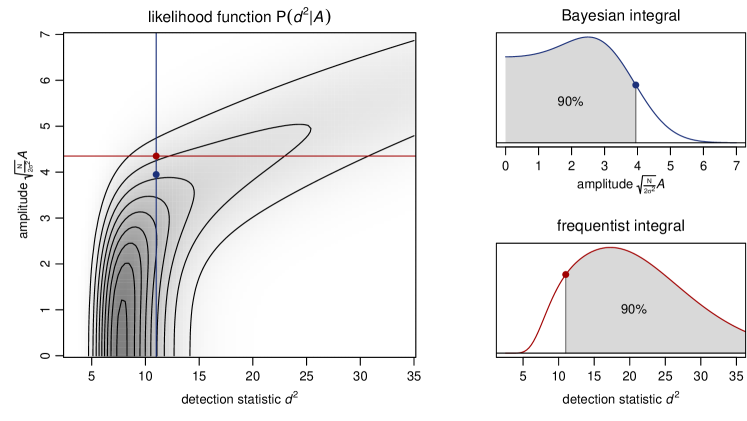
Figure 1: The integrals to be computed for a frequentist and a Bayesian 90% upper limit are very different. The Bayesian integral is computed along the vertical amplitude axis, conditioning on the observed detection statistic value $d^{2}=d^{2}_{0}$. The frequentist integral goes along the horizontal axis of possible realisations of $d^{2}$ for any given amplitude. (Example values here: $N=100$, $\Delta_{t}=1$, $\sigma^{2}=1$, $k=49$, $d^{2}_{0}=11$.)

4 Bayesian approach

We assume uniform prior distributions on phase, frequency, and amplitude. Given the (3-dimensional) likelihood function [7], one can then derive joint and marginal posterior distributions $\mathrm{P}(A,\phi,f\,|\,y)$ and $\mathrm{P}(A|y)$. However, Monte Carlo simulations show that — in this particular model — the amplitude’s marginal posterior distribution is virtually unaffected by whether one considers the complete data $y$, or only the “loudest event” $d^{2}$. The essential information about the signal amplitude is contained in that loudest event, and the marginal amplitude posterior is dominated by the conditional distribution of the loudest frequency bin. We find that the main difference between the two kinds of limits in this model is not due to maximization vs. integration of the posterior; in the following we will therefore consider only the simpler, directly comparable, and more illustrative case of a Bayesian loudest event limit based on $\mathrm{P}(A|d^{2})$ instead of $\mathrm{P}(A|y)$.

Our relevant observable now is the “loudest event” $d^{2}$. The likelihood function $\mathrm{P}(d^{2}|A)$ was defined through (5) in the previous section. The 90% upper limit on the amplitude is given by the amplitude $A^{\star}$ for which $\int_{0}^{A^{\star}}p(A\,|\,d^{2},H_{1})\,\mathrm{d}A=90\%$, so that $\mathrm{P}(A<A^{\star}\,|\,d^{2},H_{1})=90\%$.

5 Comparison

The likelihood function here is a function of two parameters: the observable $d^{2}$ and the amplitude parameter $A$. Since the amplitude prior is assumed uniform, the posterior distribution is simply proportional to the likelihood, which allows for a nice comparison of both approaches. fig:integration illustrates the integrations performed for both the frequentist and the Bayesian upper limits for some particular realisation $d^{2}=d^{2}_{0}$.

Since the data $y$ are reduced to a single observable $d^{2}$, there also is a one-to-one mapping from $d^{2}$ to the upper limit $A^{\star}$. fig:mapping shows both resulting upper limits as a function of the “loudest event” $d^{2}$.

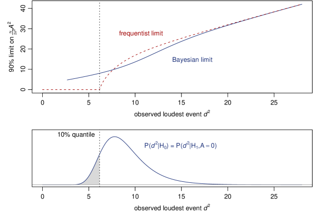
Figure 2: The mapping from observable $d^{2}$ to the upper limit on amplitude. The bottom panel shows the “background” distribution of $d^{2}$ under $H_{0}$. (Example values here: $N=100$, $\Delta_{t}=1$, $\sigma^{2}=1$, $k=49$.)

An important feature to note is that the frequentist limit will be zero for certain values of $d^{2}$. The point at (and below) which this happens is the lower 10% quantile of the “background” distribution of $d^{2}$ under $H_{0}$ (4) — at this point the probability of observing a larger $d^{2}$ value is (by definition) 90% for zero-amplitude signals already, which makes zero the 90% upper limit. Note that this implies that if $H_{0}$ in fact is true, 10% of all 90% upper limits will be zero. Note also that this is consistent with the intended 90% coverage of frequentist confidence bounds — if the upper limit is supposed to fall above and below the true amplitude value with 90% and 10% probabilities respectively, then 10% of the upper limits must be zero under $H_{0}$.

Having the distribution of the detection statistic (equations (4), (5)) and the mapping from $d^{2}$ to upper limit (fig:mapping) allows us to derive the distribution of upper limits for given parameters. [b] 3 illustrates the behaviour of the resulting upper limits for different values of amplitude $A$ and trials factor $k$. The left panel shows that for large amplitudes the two limits behave roughly the same, as one could already see from fig:mapping, while for low amplitudes the posterior upper limit will level off and will not rule out amplitude values below a certain noise level. The frequentist limit’s distribution on the other hand reaches all the way down to zero, and in particular the 90% limit’s 10% quantile follows a straight line of slope 1 and intercept 0 — the frequentist 90% limit is (by construction) essentially a statistic that has its 10% quantile at the true amplitude value.

The right panel of fig:limitdistns shows the differing behaviour of both limits as a function of the trials factor $k$ when the true amplitude is zero. The frequentist limit’s 10% quantile remains at zero (the true value), while the posterior limit is bounded away from zero but otherwise tends to yield tighter constraints on the amplitude, especially for large $k$.

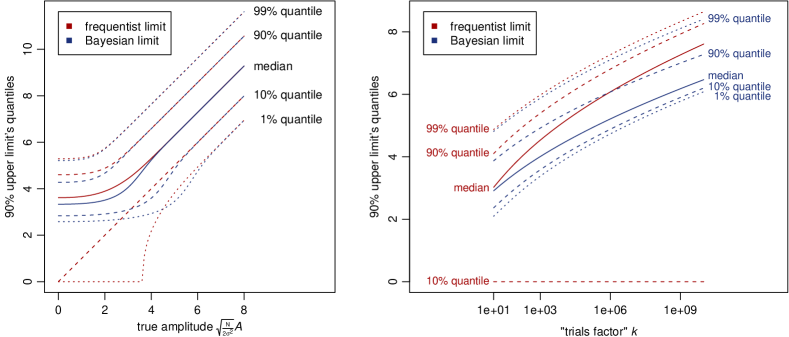
Figure 3: The distribution of upper limits as a function of amplitude (left panel) and trials factor (for zero amplitude; right panel). Note that the frequentist 90% limit is essentially a statistic that is designed to have its 10% quantile at the true amplitude value.

6 Conclusions

The most obvious technical difference between frequentist vs. Bayesian upper limits is in maximization vs. integration over parameter space. This, however, is not — at least in the example discussed here — the primary origin of discrepancies between the two. When founding both limits on maximization (i.e., the “loudest event”), the behaviour of the Bayesian limit is affected very little; so the crucial information about the signal amplitude is in fact contained in the loudest event. Both kinds of upper limits behave very similarly for “loud” signals, i.e., a large signal-to-noise ratio (SNR), but their differences become apparent in the interesting case of (near-) zero amplitude signals. While the Bayesian upper limit expresses what amplitude values may be ruled out with 90% certainty based on the data (and model assumptions), the frequentist upper confidence limit is defined solely through its “coverage” property. The frequentist 90% limit needs to end up above and below the true amplitude value with 90% and 10% probability respectively, which simply means that the frequentist limit may be any random variable that has its 10% quantile at the true amplitude. This in particular implies that for a true amplitude of $A=0$ the limit has a 10% chance of being zero as well, and it makes the frequentist limit very hard to actually interpret, not only if it actually happens to turn out as zero. When considering the effect of the trials factor (or look-elsewhere effect) in the low-SNR regime where both limits behave differently, the posterior-based limit will usually yield tighter constraints especially for large trials factors, but it will never be zero.

The Bayesian upper limit based on the amplitude’s posterior distribution will of course change with changing prior assumptions. For simplicity, we assumed an (improper) uniform amplitude prior here, but this should actually be a conservative choice in some sense, for a realistic prior in the continuous gravitational-wave context would in general be much more concentrated towards low amplitude values (something like the — also improper — prior with density $p(A)\propto\frac{1}{A^{4}}$).

Another question is how exactly one would do the actual computations for a Bayesian upper limit in practice — the frequentist upper limits are usually not computed via direct analytical or numerical integration of the likelihood, but the integral (see fig:integration) is determined in a nonparametric fashion via Monte Carlo integration and bootstrapping of the data. While the frequentist limit requires finding the amplitude $A^{\star}$ at which the integral ($\mathrm{P}(d^{2}>d^{2}_{0}\,|\,A=A^{\star})$) yields the desired confidence level, an analogous procedure to derive the Bayesian upper limit would probably require Monte Carlo sampling of $\mathrm{P}(d^{2}|A)$ across the range of all amplitudes $A$ in order to then do the integral in the orthogonal direction.

Further complications arise especially for the frequentist limit when the signal model gets more complex. The general procedure required for the Bayesian upper limit is rather obvious — determine the marginal posterior distribution of amplitude $\mathrm{P}(A|y)$, then determine the 90% quantile. The frequentist procedure on the other hand may run into major problems. For example, if there are multiple parameters affecting the signal’s SNR, a “loudest event” might be hard to define, or to translate into a constraint on the amplitude. As there may not be a simple one-to-one connection between SNR and amplitude parameter as in the present case, the “loudest event” may not be the only relevant figure to constrain the signal amplitude. The consideration of nuisance parameters is generally tricky in a frequentist framework and may effectively suggest the use of a Bayesian procedure instead [8]. Computation also becomes more complicated if the frequency parameter is not restricted to (“independent”) Fourier frequencies. Note that the reasoning behind the generalized likelihood ratio approach (see Sec. 3) leading to the “loudest event” concept was very much an ad-hoc construction in the first place.

Another notable related concept is that of a power constrained upper limit. In search experiments, these may be based on the sensitivity of the search procedure. In case the search yielded no detection, one can state the signal amplitude that would have been detected with 90% probability; this number may then also be used as a lower bound on the frequentist limit (“don’t rule out what you wouldn’t be able to detect”). However, this kind of statement requires the specification of another, additional parameter: the corresponding false alarm rate defining the threshold of what is considered a “detection”, and as such is inseparably connected to the detection procedure (see also fig:sensitivity). In particle physics a different approach is commonly taken; here the sensitivity is usually specified as the expected upper limit for many repetitions of the experiment in the absence of a signal. This figure would correspond to the solid lines at zero amplitude in Fig. 3. An important point to note is that both these sensitivity statements do not depend on the observed data.

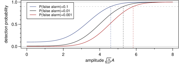
Figure 4: Illustration of the determination of a 90% detection sensitivity threshold. Such a statement would be independent of the observed data, and it requires the specification of an additional parameter: the corresponding false alarm rate defining the threshold of what is considered a “detection”. (Here: $N=100$, $\Delta_{t}=1$, $\sigma^{2}=1$, $k=49$.)

References

- [1] B. Abbott et al. Setting upper limits on the strength of periodic gravitational waves from PSR J1939+2134 using the first science data from the GEO 600 and LIGO detectors. Physical Review D, 69(8):082004, April 2004.
- [2] P. Brady, J. D. E. Creighton, and A. G. Wiseman. Upper limits on gravitational-wave signals based on loudest events. Classical and Quantum Gravity, 21(20):S1775–1781, October 2004.
- [3] A. Gelman, J. B. Carlin, H. Stern, and D. B. Rubin. Bayesian data analysis. Chapman & Hall / CRC, Boca Raton, 1997.
- [4] B. P. Abbott et al. Searches for gravitational waves from known pulsars with science run 5 LIGO data. The Astrophysical Journal, 713(1):671–685, April 2010.
- [5] A. M. Mood, F. A. Graybill, and D. C. Boes. Introduction to the theory of statistics. McGraw-Hill, New York, 3rd edition, 1974.
- [6] L. A. Wainstein and V. D. Zubakov. Extraction of signals from noise. Prentice-Hall, Englewood Cliffs, NJ, 1962.
- [7] G. L. Bretthorst. Bayesian spectrum analysis and parameter estimation, volume 48 of Lecture Notes in Statistics. Springer-Verlag, Berlin, 1988.
- [8] A. C. Searle. Monte-Carlo and Bayesian techniques in gravitational wave burst data analysis. Arxiv preprint 0804.1161 [gr-qc], April 2008.