Floridian high-voltage power-grid network partitioning and cluster optimization using simulated annealing

Abstract

Many partitioning methods may be used to partition a network into smaller clusters while minimizing the number of cuts needed. However, other considerations must also be taken into account when a network represents a real system such as a power grid. In this paper we use a simulated annealing Monte Carlo (MC) method to optimize initial clusters on the Florida high-voltage power-grid network that were formed by associating each load with its “closest” generator. The clusters are optimized to maximize internal connectivity within the individual clusters and minimize the power deficiency or surplus that clusters may otherwise have.

1 Introduction

The lack of a pre-planned strategy for splitting a power-grid system into separate parts with self-sufficient power generation is one of the reasons for large-scale blackouts that have devastating effects on the economy and welfare of any modern society [1, 2]. This defensive strategy (intentional islanding) is effective in preventing cascading outages [2, 3].

Multiple approaches to intentional islanding (see, e.g., [1, 2, 3, 4, 5, 6, 7]) have been suggested for optimizing the selection of the lines to be cut. These studies can be based on the analysis of the system topology based on a representation of the network as a graph [8, 9, 10, 11]. Some topologies are easier to split into islands than others. The identification of “weak” links and their removal can split a given topology into independent islands. While many of the above approaches are very good at the identification of “weak” links, the resulting clusters or islands are usually not optimized for other qualities such as generating capacity.

Here we present a study utilizing a matrix method for intentional islanding of a utility power grid. The method uses a Monte Carlo (MC) simulated annealing [12] technique for optimizing the resulting islands’ internal connectivity as well as balancing their generating capacity. The concept is illustrated by application to the Floridian high-voltage power grid.

2 Methods

The quality of a particular partitioning of a graph into $M$ communities, ${\mathcal{C}}=\{C_{1},...,C_{M}\}$ can be estimated by Newman’s modularity [10]. It compares the proportion of edges that are internal to a community in the particular graph with the same proportion in an average null-model. It is defined as follows:

$$Q=\frac{1}{w}\sum_{ij}\left(w_{ij}-\frac{w_{i}w_{j}}{w}\right)\delta\left(C(i),C(j)\right)\;,$$ (1)

where $\delta\left(C(i),C(j)\right)=1$ if nodes $i$ and $j$ belong to the same community, and $0$ otherwise. Ideally, one would like to maximize $Q$ while partitioning a power-grid network. This will ensure that the different communities are well connected internally. Moreover, one would like to minimize the generating power surplus or deficiency over all the clusters. Here we will use a partitioning scheme consistent with a power-grid network and try to optimize the resulting clusters for internal connectivity and power self-sufficiency using a Monte Carlo simulated annealing approach. The resulting set of clusters form a new network (in a renormalization-group sense) where each cluster is represented by a node on the new network. The islanding procedure and MC optimization are repeated until some required criteria are met.

2.1 Partitioning

We use a simplified representation of the power grid as an undirected graph [8, 10] defined by the $N\times N$ symmetric conductivity matrix $\bf W$, whose elements $w_{ij}\geq 0$ represent the “conductivities” of the edges (transmission lines) between vertices (generators or loads) $i$ and $j$,

$$w_{ij}=\frac{{\rm number\,of\,lines\,between\,vertices\,}i\,{\rm and}\,j}{\rm{\,normalized\,geographical\,distance}},$$ (2)

where the “geographical distance” is the length of the edge connecting nodes $i$ and $j$, and is normalized by the minimum geographical distance between two nodes over the whole network.

The row sums of $\bf W$ define the diagonal matrix $\bf D$. Graph analysis can be performed using one of several matrices derived from $\bf W$. The Laplacian, ${\bf L}={\bf D}-{\bf W}$, is a symmetric matrix with vanishing row sums. It embodies Kirchhoff’s laws and thus represents a simple resistor network with conductances $w_{ij}$. Multiplied by a column vector $|\phi\rangle$ of vertex potentials, it yields the vector of currents entering the circuit at each vertex, ${\bf L}|\phi\rangle=|I\rangle$. This equation can be rewritten as ${\bf L}^{(-1)}|I\rangle=|\phi\rangle$, where ${\bf L}^{(-1)}$ is the pseudo-inverse of the Laplacian. In other words, given a current vector, defined as being positive at generator nodes and negative at load nodes, one can calculate the potential vector $|\phi\rangle$. Using this potential vector and the matrix $\bf W$, we calculate the network-current matrix $\bf K$, whose elements are the currents between the corresponding nodes: ${k}_{ij}=(\phi_{j}-\phi_{i}){w}_{ij}$. Additionally using the matrix ${\bf L}^{(-1)}$, one can calculate an effective distance or equivalent resistance ${\bf R}$ between any two nodes [13]: $({\bf R})_{ij}=({\bf L}^{(-1)})_{ii}+({\bf L}^{(-1)})_{jj}-2({\bf L}^{(-1)})_{ij}$. Consequently, given a current vector and a conductivity matrix ${\bf W}$, the network-current matrix ${\bf K}$ and the equivalent resistance matrix ${\bf R}$ can be evaluated. In this paper we use these two last matrices to achieve an initial partitioning of the Floridian high-voltage grid.

The goal is to partition the power grid into communities of vertices that are highly connected internally, but only sparsely connected to the rest of the network. For the islanding to be useful, each island should contain at least one generating plant. To accomplish this, we use a clustering algorithm where each load $i$ is connected to the “nearest” generator $j$. The nearest generator $j$ is the one located “upstream” from load $i$, i.e. $\phi_{j}>\phi_{i}$, and for which $({\bf R})_{ij}$ is minimum. The Floridian high-voltage grid [14] at this first level of islanding is shown in figure 1(a).

Kirchhoff’s junction law, when applied at each node, tells us that the sum of all network currents going in and out of node $i$ is equal to $|I\rangle_{i}$. Thus we can think of $|I\rangle_{i}$ as the current provided by a generator at node $i$ if it is positive, or consumed by a load if it is negative. Moreover, given the constant voltage rating (138, 230, 345, … kV), $|I\rangle_{i}$ becomes proportional to the power being generated or consumed at node $i$. This means that we can choose our initial current vector proportional to the generating power of each power plant. Since the actual power rating for power plants on the grid was not available to us, we here assume that each generator’s power is proportional to the number of edges linking to it, or its degree. The current vector component at each node $i$ is then defined as $|I\rangle_{i}=\frac{{\rm degree}_{i}}{\sum_{\rm generators}{\rm degree}_{j}}\,{\rm for\,generators}$ and $|I\rangle_{i}=-\frac{{\rm degree}_{i}}{\sum_{\rm loads}{\rm degree}_{j}}\,{\rm for\,loads}$.

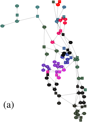
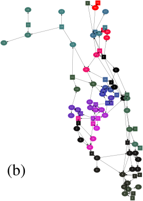
Figure 1: (a) Florida high-voltage power grid partitioned by connecting loads (ovals) to their “nearest” generators (squares). (b) Grid clustering after the MC simulated annealing algorithm is used for optimizing modularity and power sufficiency of the partitioned network shown in (a). Nodes of the same color and label belong to the same cluster. See text for discussion.

2.2 Monte Carlo

Since the power generation or consumption rate of any generator or load is directly proportional to its current-vector component $|I\rangle_{i}$, a community’s total generating surplus or deficiency is proportional to the sum of its members’ current-vector components. Thus, to optimize our partitioning for well-balanced communities, we try to minimize the variance of the new current vector $|\tilde{I}\rangle$, whose components are defined as $|\tilde{I}\rangle_{i}=\sum_{i\geq j}|I\rangle_{j}\delta(C(i),C(j))$ after each iteration of the islanding procedure. We need to maximize the modularity $Q$ for better internal connectivity at the same time. For this purpose, we define an optimization parameter

$$E=\frac{Q}{Q_{\rm init}}-\sqrt{\frac{VAR(|\tilde{I}\rangle)}{VAR(|\tilde{I}\rangle_{\rm init})}},$$ (3)

where the subscript “init” designates the initial value after recombination, but before any MC steps. This form gives equal emphasis on optimizing modularity and load balance. More emphasis could be given to the optimization of one quantity versus the other by multiplying the term corresponding to it by some weighting factor.

The MC process proceeds as follows. First, a load node $i$ is selected at random. Then, if $i$ is at the edge of the cluster it belongs to, i.e, if it is connected to a neighboring cluster, we randomly select one of the neighboring clusters connected to $i$ and attempt to move this load to that neighboring cluster. If this move does not break the first cluster into two disconnected parts, the move is accepted with a Metropolis acceptance rate [15] $R=\min(1,e^{(-\beta\Delta E)})$, where $\Delta E=E_{a}-E_{i}$ is the difference between the attempted state and the initial state for that move, and $\beta$ is an “inverse temperature.” In a fashion similar to simulated annealing, we start at a high temperature and gradually decrease it to zero while saving the configuration for which $E$ is maximum. This process is repeated to look for the global maximum of $E$.

2.3 Recombination

After the initial partitioning and MC, the number of clusters produced is equal to the number of the generators in the circuit (Fig. 1(a)), as expected from our clustering scheme. A new network can be constructed from this group of clusters by regarding each cluster as a new node. The connections between the new nodes are the same as the connections between the previous clusters. This defines a new network with new connections and a new conductivity matrix. The current vector defined above, $|\tilde{I}\rangle$, is the new current vector because its components represent the generating surplus or deficiency of each of the old clusters or new “super-generators” or “super-loads,” respectively. Given the new network and the new current vector, we repeat the above partitioning and MC schemes on the new network. The number of clusters at this stage is equal to the number of “super-generators.” This process of recombination is repeated to look for the optimum configuration until all the original nodes belong to one cluster. The optimization parameter ${\it vs.}$ MC step and the corresponding modularity are shown in figure 2, where the red circles are the values of $Q$ for maximum $E$ at each level of recombination.

3 Results and Conclusion

The map of the Floridian high-voltage grid [14] is a network with 84 vertices, 31 of which are generating plants. We have modeled it as an undirected graph with 137 edges. The conductivities were calculated according to equation (2).

While figure 1(a) shows the clusters resulting from the first partitioning scheme, figure 1(b) shows the same network after the MC annealing procedure is performed. The current vector and the corresponding modularity before and after the MC annealing are shown in figure 3. As can be seen, the MC process narrows the spread of the current values or in other words, the average power surplus or deficiency for the clusters is smaller. Moreover, while the modularity starts at a value of $0.33$, it ends at a value of $0.47$ after MC optimization and before the first recombination. The maximum optimization parameter, $E_{\rm max}=1.33$ with a corresponding $Q=0.63$ was achieved shortly after the first recombination. Comparable values ($E=1.31$ and $Q=0.62$) are obtained in the second iteration.

While many methods can be used to partition a network into smaller clusters, there remains the need for further optimization of the resulting cluster properties. Here we have used a clustering procedure to partition the Floridian power-grid network that takes into account the generating power of each of the power plants. Moreover, we have used MC simulated annealing to optimize the resulting clusters for better internal connectivity and power self-sufficiency.

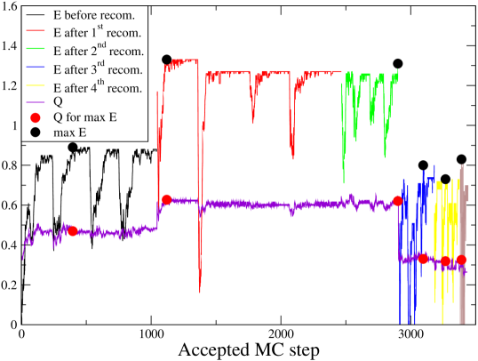
Figure 2: Modularity Q and the optimization parameter $E$ ${\it vs.}$ MC step.

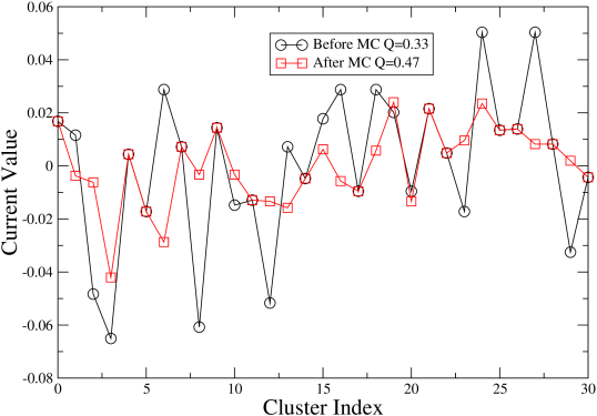
Figure 3: Components of the current vector $|\tilde{I}\rangle$ vs. the cluster index. It can be seen that the MC procedure narrows the spread of the current values, meaning that, on average, the individual clusters are closer to self-sufficiency than before MC. The legend shows the significant improvement in modularity.

References

- [1] H. Li, G. W. Rosenwald, J. Jung, C. Liu, Strategic power infrastructure defense, Proc. IEEE 93 (2005) 918–933.
- [2] A. Peiravi, R. Ildarabadi, A fast algorithm for intentional islanding of power systems using the multilevel kernel -means approach, J. Appl. Sci. 9 (2009) 2247–2255.
- [3] B. Yang, V. Vittal, G. T. Heydt, Slow-coherency-based controlled islanding – a demonstration of the approach on the august 14, 2003 blackout scenario, IEEE Trans. Power Syst. 21 (2006) 1840–1847.
- [4] G. Karypis, V. Kumar, Multilevel -way partitioning scheme for irregular graphs, J. Parallel Distr. Computing 48 (1998) 96–129.
- [5] S. P. Chowdhury, S. Chowdhury, C. F. Ten, P. A. Crossley, Islanding protection of distribution systems with distributed generators – a comprehensive survey report, in: Proceedings of Power and Energy Society General Meeting - Conversion and Delivery of Electrical Energy in the 21st Century, IEEE, 2008.
- [6] X. Wang, V. Vittal, System islanding using minimal cutsets with minimum net flow, in: 2004 IEEE PES Power Systems Conference and Exposition, vol. 1, IEEE, 2004, pp. 379–384.
- [7] Y. Liu, Y. Liu, Aspects on power system islanding for preventing widespread blackout, in: Proceedings of the 2006 IEEE International Conference on Networking, Sensing and Control, ICNSC’06, Ft. Lauderdale, FL, IEEE, 2006, pp. 1090–1095.
- [8] A. J. Seary, W. D. Richards, Spectral methods for analyzing and visualizing networks: An introduction, in: R. A. Breiger (Ed.), Dynamic Social Network Modeling and Analysis, National Academies’ Press, Washington, DC, 2003.
- [9] S. Fortunato, Community detection in graphs, Phys. Rep. 486 (2010) 75–174.
- [10] M. E. J. Newman, Analysis of weighted networks, Phys. Rev. E 70 (2004) 056131.
- [11] I. Abou Hamad, B. Israels, P. A. Rikvold, and S. V. Poroseva. Spectral Matrix Methods for Partitioning Power Grids: Applications to the Italian and Floridian High-voltage Networks, in: D. P. Landau, S. P. Lewis, and H.-B. Schüttler (Ed.), Computer Simulation Studies in Condensed-Matter Physics XXIII (CSP10), Physics Procedia 4, (2010) 125–129.
- [12] S. Kirkpatrick, C. D. Gelatt and M. P. Vecchi, Optimization by Simulated Annealing, Science, New Series 220 (1983) 671–680.
- [13] D. J. Klein, M. Randić, Resistance Distance, J. Math. Chem. 12 (1993) 81.
- [14] S. Dale, T. Alquthami, T. Baldwin, O. Faruque, J. Langston, P. McLaren, R. Meeker, M. Steurer, K. Schoder, Progress Report for the Institute for Energy Systems, Economics and Sustainability and the Florida Energy Systems Consortium, Florida State University, Tallahassee, FL, 2009.
- [15] D. P. Landau, K. Binder, A Guide to Monte Carlo Simulations in Statistical Physics. Cambridge Univ. Press, Cambridge, 2000.