Sub-Poissonian fluctuations in a 1D Bose gas: from the quantum quasi-condensate to the strongly interacting regime

Abstract

We report on local, in situ measurements of atom number fluctuations in slices of a one-dimensional Bose gas on an atom chip setup. By using current modulation techniques to prevent cloud fragmentation, we are able to probe the crossover from weak to strong interactions. For weak interactions, fluctuations go continuously from super- to sub-Poissonian as the density is increased, which is a signature of the transition between the sub-regimes where the two-body correlation function is dominated respectively by thermal and quantum contributions. At stronger interactions, the super-Poissonian region disappears, and the fluctuations go directly from Poissonian to sub-Poissonian, as expected for a ‘fermionized’ gas.

Fluctuations witness the interplay between quantum statistics and interactions and therefore their measurement constitutes an important probe of quantum many-body systems. In particular, measurement of atom number fluctuations in ultracold quantum gases has been a key tool in the study of the Mott insulating phase in optical lattices Folling2005 , isothermal compressibility of Bose and Fermi gases Esteve06 ; Armijo10_2 ; Sanner10 ; Mueller10 , magnetic susceptibility of a strongly interacting Fermi gas Sanner2011 , scale invariance of a two-dimensional Bose gas Hung2011 , generation of atomic entanglement in double-wells Esteve2008 , and relative number squeezing in pair-production via binary collisions Jaskula2010 ; TwinAtomBeams .

While a simple account of quantum statistics can change the atom number distribution, in a small volume of an ideal gas, from a classical-gas Poissonian to super-Poissonian (for bosons) or sub-Poissonian (for fermions) distributions, many-body processes can further modify the correlations and fluctuations. For example, three-body losses may lead to sub-Poissonian fluctuations in a Bose gas Whitlock2010 ; Itah2010 . Even without dissipation, the intrinsic interatomic interactions can also lead to sub-Poissonian fluctuations, such as in a repulsive Bose gas in a periodic lattice potential, where the energetically costly atom number fluctuations are suppressed. This effect has been observed for large ratios of the on-site interaction energy to the inter-site tunnelling energy Wei2007 ; Gross2010 , with the extreme limit corresponding to the Mott insulator phase  Bakr2010 ; Sherson2010 . The same physics, accounts for sub-Poissonian fluctuations observed in double-well experiments Sebby-Strabley2007 ; Esteve2008 . Sub-Poissonian fluctuations of the total atom number have been also realised via controlled loading of the atoms into very shallow traps  Chuu2005 .

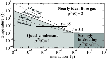
Figure 1: Phase diagram in the interaction-temperature parameter space of a repulsive uniform 1D Bose gas Kheruntsyan05 . The values of the local two-body correlation $g^{(2)}(0)$ are indicated for the three main regimes (white and grey areas). The two horizontal lines show the parameters explored in this paper.

In this work, we observe for the first time sub-Poissonian atom number fluctuations in small slices of a single one-dimensional (1D) Bose gas with repulsive interactions, where each slice approximates a uniform system. Taking advantage of the long scale density variation due to a weak longitudinal confinement, we monitor – at a given temperature – the atom number fluctuations in each slice as a function of the local density. For a weakly interacting gas, the measured fluctuations are super-Poissonian at low densities, and they become sub-Poissonian as the density is increased and the gas enters the quantum quasi-condensate sub-regime that is dominated by quantum rather than thermal fluctuations (see Fig. 1, with the interaction and temperature parameters, $\gamma$ and $t$, defined below). When the strength of interactions is increased, the fluctuations are no longer super-Poissonian at low densities and remain sub-Poissonian at high densities. The absence of super-Poissonian behavior implies that the gas enters the strongly interacting regime where the repulsive interactions between bosonic atoms mimic fermionic Pauli blocking, and the quantities involving only densities are those of an ideal Fermi gas. Our results in all regimes are in good agreement with the exact Yang-Yang thermodynamic solution for the uniform 1D Bose gas with contact interactions YangYang69 .

We recall that the thermodynamics of a uniform 1D Bose gas can be characterized by the dimensionless interaction and temperature parameters, $\gamma\!=\!mg/\hbar^{2}n$ and $t\!=\!2\hbar^{2}k_{B}T/mg^{2}$ Kheruntsyan05 , where $T$ is the temperature, $n$ the 1D density, $g\simeq 2\hbar\omega_{\perp}a$ is the coupling constant, $a$ is the $s$-wave scattering length, and $\omega_{\perp}$ is the frequency of the transverse harmonic confining potential. Figure 1 shows the different regimes of the gas, characterized by the behavior of the two-body correlation function $g^{(2)}$ and separated by smooth crossovers Kheruntsyan05 . Of particular relevance to the present work are the quantum quasi-condensate sub-regime where $g^{(2)}(0)\lesssim 1$ Kheruntsyan05 , and the strongly interacting regime where $g^{(2)}(0)\ll 1$ Kheruntsyan05 ; Weiss2005 . The two different situations studied in this work are shown in Fig. 1 by two horizontal lines at different values of $t$.

The experiments are performed using ⁸⁷Rb atoms ($a\!=\!5.3$ nm) confined in a magnetic trap realised by current-carrying microwires on an atom chip. For the data at $t=65$, as in Ref. Armijo10_2 , we use an H-shaped structure to realise a very elongated harmonic trap at $\sim\!\!100~{}\mu$m away from the wires, with the longitudinal frequency $\omega_{\parallel}/2\pi\!=\!5.5$ Hz and $\omega_{\perp}/2\pi\!=\!3.3$ kHz. Using rf evaporation we produce clouds of $\sim\!\!3000$ atoms in thermal equilibrium at $T\!=\!16.5~{}$nK, corresponding to $t\!=\!65$. We extract the longitudinal density profile from in situ absorption images as detailed in ArmijoSkew . The local atom number fluctuations in the image pixels, whose length in the object plane is $\Delta=4.5~{}\mu$m, are measured by repeating the same experiment hundreds of times and performing statistical analysis of the density profiles Armijo10_2 . For each profile and pixel, we record the atom number fluctuation $\delta N=N-\langle N\rangle$, where $\langle N\rangle=n\Delta$ is the mean atom number. The results are binned according to $\langle N\rangle$ and for each bin we compute the variance $\langle\delta N^{2}\rangle$. The contribution of optical shot noise to $\langle\delta N^{2}\rangle$ is subtracted.

Figure 2 shows the measured variance $\langle\delta N^{2}\rangle$ versus $\langle N\rangle$. Since $l_{c}\ll\!\max\{\Delta,d\}\!\ll\!L$ in our experiment, where $L\!\simeq\!50$ $\mu$m is the cloud rms length, $d$ is the imaging resolution, and $l_{c}$ is the correlation length of density fluctuations Kheruntsyan05 ; Deuar2009 , the local density approximation is expected to correctly describe both the average density profile and the fluctuations Kheruntsyan05 ; Armijo10_2 . Accordingly, $\langle\delta N^{2}\rangle$ is expected to follow the thermodynamic prediction Armijo10_2 ; ArmijoSkew

$$\langle\delta N^{2}\rangle=\kappa k_{B}T\Delta(\partial n/\partial\mu)_{T},$$ (1)

where $n(\mu,T)$ is the linear density of a homogeneous gas, and $\mu$ is the chemical potential. The reduction factor $\kappa$ accounts for the finite resolution of the imaging system; it is determined from the measured correlation between adjacent pixels ArmijoSkew , from which we deduce the rms width of the imaging impulse response function $\cal A$ (assumed to be Gaussian), and find that $d=3.5$ $\mu$m and $\kappa=0.34$.

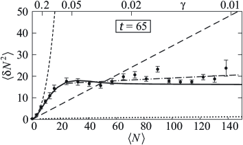
Figure 2: Variance of the atom number fluctuations in a weakly interacting gas, for $t=65$. The measured data are shown as circles together with statistical uncertainties. Predictions from Eq. (1) and different thermodynamic models are shown as solid (Yang-Yang), short-dashed (ideal Bose gas) and dash-dotted (quasi-condensate) lines. The long-dashed line is the Poissonian limit and the low lying dotted line is the contribution from quantum fluctuations. Here $\omega_{\perp}/2\pi\!=\!3.3$ kHz, $\omega_{\parallel}/2\pi\!=\!5.5$ Hz, $T\!=\!16$ nK ($k_{B}T=\!0.1\hbar\omega_{\perp}$), and $\kappa=0.34$.

The thermodynamic predictions for an ideal Bose gas and a quasi-condensate are shown in Fig. 2. In the quasi-condensate regime we use the equation of state $\mu=\hbar\omega_{\perp}(\sqrt{1+4na}-1)$ Fuchs03 . The temperature is obtained by fitting the quasi-condensate prediction to the measured fluctuations at high densities. Usual features of the quasi-condensation transition are seen Armijo10_2 : at low density, the gas lies within the ideal gas regime where, for degenerate gases, bosonic bunching raises the fluctuations well above the Poissonian limit; at high density the gas lies in the quasi-condensate regime where interactions level off the density fluctuations. Within the quasi-condensate regime, the fluctuations go from super-Poissonian to sub-Poissonian, with $\langle\delta N^{2}\rangle/\kappa\langle N\rangle$ going from $2$ to $0.44$. Using the approximate 1D expression $\mu\!=\!gn$, Eq. (1) shows that the transition from super- to sub-Poissonian behavior occurs at $k_{B}T\!\simeq\!gn$, which is the boundary between the thermal and quantum quasi-condensate regimes Kheruntsyan05 ; Deuar2009 . The fluctuations in the whole explored density domain are in good agreement with the exact 1D Yang-Yang predictions. The small discrepancy at  high densities between the Yang-Yang and the quasi-condensate models is due to the transverse swelling of the cloud  ArmijoSkew ; Armijo10_2 . In the following, we neglect this 3D effect and perform a purely 1D analysis.

Going beyond the thermodynamic relation (1), the variance $\langle\delta N^{2}\rangle$ in a pixel is given by

$$\langle\delta N^{2}\rangle=\!\!\int\!\!d^{4}{\cal{Z}}~{}\langle\delta n(z)\delta n(z^{\prime})\rangle\;{\cal A}(z-Z){\cal A}(z^{\prime}-Z^{\prime}),$$ (2)

where $\int\!d^{4}{\cal{Z}}\equiv\!\!\int_{0}^{\Delta}\!\!dZ\!\!\int_{0}^{\Delta}\!\!dZ^{\prime}\!\!\int_{-\infty}^{\infty}\!\!dz\!\!\int_{-\infty}^{\infty}\!\!dz^{\prime}$, $\delta n(z)=n(z)-\langle n(z)\rangle$ is the density fluctuation, and $\int_{-\infty}^{+\infty}\!dZ{\cal A}(Z)\!=\!1$. Isolating the one- and two-body terms, one has

$$\langle\delta n(z)\delta n(z^{\prime})\rangle=n\delta(z-z^{\prime})+n^{2}[g^{(2)}(z-z^{\prime})-1].$$ (3)

The first term, when substituted into Eq. (2), accounts for Poissonian level of fluctuations, $\kappa\langle N\rangle$. Therefore, the measured sub-Poissonian fluctuations in Fig. 2 imply that $g^{(2)}(z-z^{\prime})-1<0$. Such anti-bunching stems from quantum fluctuations. Indeed, within the Bogoliubov approximation, valid for quasi-condensates, one has Deuar2009

$$g^{(2)}(z\!-\!z^{\prime})-1\!=\int\frac{dk}{2\pi n}\left[2n_{k}f_{k}-(1-f_{k})\right]e^{ik(z-z^{\prime})},$$ (4)

where $f_{k}=1/\sqrt{1+4/(l_{\xi}k)^{2}}$ and $n_{k}=1/\left(e^{\epsilon_{k}/k_{B}T}-1\right)$ is the thermal occupation of the Bogoliubov collective mode of wavenumber $k$ and energy $\epsilon_{k}=\hbar^{2}k^{2}/(2m\sqrt{1+4/(l_{\xi}k)^{2}})$, with $l_{\xi}=\hbar/\sqrt{mgn}$ being the healing length. The first term in the rhs of Eq. (4) which accounts for thermal fluctuations is positive, whereas the second term which is the contribution of quantum (i.e., zero temperature) fluctuations is negative Deuar2009 . Therefore, the negativity of $g^{(2)}(z-z^{\prime})-1$ implies that the quantum fluctuations give a larger contribution to $g^{(2)}(z-z^{\prime})-1$ than the thermal ones.

It should be emphasised, however, that the quantity we measure is $\langle\delta N^{2}\rangle$, and as we show below, for our large values of $\Delta$ and $d$ it is still dominated by thermal (rather than quantum) fluctuations. This is because the contribution to $\langle\delta N^{2}\rangle$ of the one-body term almost cancels out the contribution of the zero-temperature two-body term. Indeed, the contribution of quantum fluctuations to $\langle\delta N^{2}\rangle$, calculated using Eqs. (2), (3), and (4), is

$$\langle\delta N^{2}\rangle_{T=0}=\frac{\langle N\rangle}{\Delta\pi}\int_{-\infty}^{\infty}dkf_{k}\frac{1-\cos(k\Delta)}{k^{2}}e^{-k^{2}d^{2}}.$$ (5)

Since $f_{k}\propto kl_{\xi}$ when $kl_{\xi}\ll 1$, we find that for $\Delta\gg l_{\xi},d$, $\langle\delta N^{2}\rangle_{T=0}$ scales as $nl_{\xi}\ln(\Delta/l_{\xi})$. On the other hand, the thermal contribution given by Eq. (1), scales as $\Delta T/g$. Therefore, the quantum contribution becomes negligible as $\Delta\rightarrow\infty$, and the thermodynamic prediction of Eq. (1) is recovered Klawunn2011 . For our parameters, the contribution of Eq. (5) to $\langle\delta N^{2}\rangle$ is shown as a dotted line in Fig. 2.

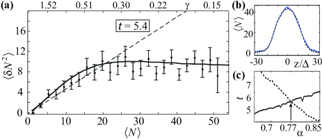
Figure 3: (a) Variance $\langle\delta N^{2}\rangle$ close to the strongly interacting regime, for $t=5.4$. Different curves are as in Fig. 2, but for $\omega_{\perp}/2\pi\!=\!18.8$ kHz, $\omega_{\parallel}\!=\!7.5$ Hz, $T\!=\!40$ nK ($k_{B}T\!=\!0.044\hbar\omega_{\perp}$), and $\kappa\!=\!0.47$. (b) Average density profile (solid line) together with the Yang-Yang prediction (dashes). (c) The value of $t$ obtained from fits to the density profile (dotted line) and atom number fluctuations (solid line) for different $\alpha$ (see text).

In weakly interacting gases, the atom number fluctuations take super-Poissonian values in the degenerate ideal gas and thermal quasi-condensate regimes, $\langle\delta N^{2}\rangle/\langle N\rangle$ reaching its maximum at the quasi-condensate transition where it scales as $t^{1/3}$ Armijo10_2 . When $t$ is decreased, the super-Poissonian zone is expected to merge towards the Poissonian limit and it vanishes when the gas enters the strongly interacting regime. This trend is exactly what we observe in Fig. 3(a), for $t\!=\!5.4$: at large densities, we see suppression of $\langle\delta N^{2}\rangle$ below the Poissonian level but, most importantly, we no longer observe super-Poissonian fluctuations at lower densities ($\langle\delta N^{2}\rangle/\kappa\langle N\rangle\!<\!1.3$ within the experimental resolution) . Interestingly, no simple analytic theory is applicable to this crossover region, and the only reliable prediction here is the exact Yang-Yang thermodynamic solution [solid line in Fig. 3(a)].

We now describe the experimental techniques that allowed us to increase significantly $\omega_{\perp}$ in order to reach $t=5.4$. Keeping a reasonable heat dissipation in the wires, increasing $\omega_{\perp}$ requires bringing the atomic cloud closer to the chip. However, using dc micro-wire currents, one would observe fragmentation of the cloud due to wire imperfections and hence longitudinal roughness of the potential Esteve2004 . To circumvent this problem, we use the modulation techniques developed in Trebbia2007 ; Bouchoule2008 . The atom chip schematic is shown in Fig. 4. The transverse confinement is realized by three wires, carrying the same ac current modulated at $200$ kHz, and a longitudinal homogeneous dc magnetic field of $\sim\!1.8$ G realized by external coils. The modulation is fast enough so that the atoms experience the time-averaged potential, transversely harmonic. Monitoring dipole oscillations we measure $\omega_{\perp}/2\pi$ varying from $2$ to $25$ kHz, for ac current amplitude varying from $40$ to $200$ mA. The longitudinal confinement, with $\omega_{z}/2\pi$ varying from $5$ to $12$ Hz, is realised by wires perpendicular to the $z$-direction, carrying dc currents of a few tens of mA. After a first rf evaporation stage in a dc trap we load $6\times 10^{4}$ atoms at a few $\mu$K in the ac trap where we perform further rf evaporation at $\omega_{\perp}/2\pi\simeq 2$ kHz and $\omega_{\parallel}/2\pi\simeq 12$ Hz. Next we lower the longitudinal trapping frequency to about $7$ Hz and then ramp up the transverse frequency to $18.8$ kHz in $600$ ms keeping the rf evaporation on during this compression. After ramping the rf power down in $100$ ms and letting the cloud to thermalize for $150$ ms, we switch off the wire currents and image the atomic cloud after $50$ $\mu$s with a $60$ $\mu$s long resonant probe pulse. The probe is circularly polarised and its intensity, chosen to optimise the signal to noise ratio, is about $0.2\,I_{\mathrm{sat}}$, where $I_{\mathrm{sat}}=1.67$ mW is the saturation intensity of the D₂ line. Finally, we get the longitudinal profile of the cloud by summing over the transverse pixels. We typically obtain clouds at $t\simeq 1-6$. Taking a few hundreds of images under the same conditions, we measure $\langle\delta N^{2}\rangle$ the same way as for the results of Fig. 2.

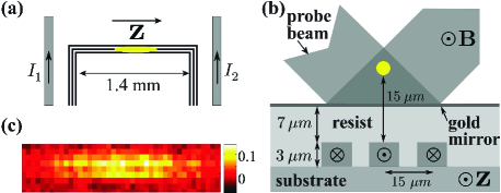
Figure 4: (color online) (a) Wire schematic of the atom chip: three gold wires along $\mathbf{Z}$ carry an ac current and produce a tight transverse confining potential. The longitudinal confinement is realized with dc currents $I_{1}$ and $I_{2}$. (b) The wires are buried under a layer of resist, which ensures electrical insulation and surface planarization. The resist is covered with 200 nm thick gold mirror that reflects the probe beam. The atoms are $15\!$ $\mu$m away from the wires and see the interference pattern produced by the probe and the reflected beam. (c) Typical optical-density image of a gas of $10^{3}$ atoms.

One crucial point to correctly determine the longitudinal profile is the knowledge of the absorption cross section $\sigma$. In our setup, atoms sit in an interference pattern during the imaging pulse [see Fig. 4(b)] and are subjected to a magnetic field so that the determination of $\sigma$ is not simple. Following Reinaudi , we assume $\sigma=\alpha\sigma_{\mathrm{o}}/\left(1+\alpha I/I_{\mathrm{sat}}\right)$, where $I$ is the intensity of the probe beam, $\sigma_{\mathrm{o}}=3\lambda^{2}/2\pi$ is the resonant cross section of the transition $|F=2,m_{F}=2\rangle\rightarrow|F^{\prime}=3,m_{F}^{\prime}=3\rangle$, and $\alpha$ is a numerical factor. Solving the optical Bloch equations (OBE) for our probe intensity and duration, we find that such a law is valid, and we obtain $\alpha=0.75$. In this calculation, we averaged $\alpha$ over the distance to the chip, which is expected to be valid as atoms diffuse over a rms width of about $1~{}\mu m$ during the imaging pulse, which is larger than the interference lattice period. The factor $\alpha$ can be also deduced from the mean density profile and/or the atom number fluctuations using the thermodynamic Yang-Yang predictions. Fitting both $\alpha$ and $t$ to either the mean profile or the fluctuations leads to strongly correlated values of $\alpha$ and $t$ but with large uncertainty in $\alpha$. Combining both pieces of information, however, enables a precise determination of $\alpha$. More specifically, using the Yang-Yang theory, we extract $t_{p}$ and $t_{f}$ from fits to the mean profile and the fluctuations, respectively, for various values of $\alpha$ [see Fig. 3(b) and (c)]. The intersection $t_{p}=t_{f}$ gives the correct value of $\alpha$. We find $\alpha=0.77$, in good agreement with the OBE calculation. The corresponding value of $t$ is $5.4$ and hence $T=40$ nK.

In summary, we have realised for the first time a single 1D Bose gas close to the strongly interacting regime. In contrast to realisations of arrays of multiple 1D gases in 2D optical lattices Phillips-2004 ; Weiss2005 , our experiments have allowed us to perform atom number fluctuation measurements in small slices of the gas, not possible with multiple 1D gases. In the weakly interacting regime, we reached the quantum quasi-condensate regime (where $k_{B}T\!<\!\mu\!=\!gn$) in a strictly 1D situation with $k_{B}T\!\ll\!\hbar\omega_{\perp}$. Although the two-body correlation function $g^{(2)}$ is dominated by quantum fluctuations in this regime, we have shown that the variance $\langle\delta N^{2}\rangle$ is still dominated by thermal excitations. To resolve quantum fluctuations one would need to access wavelengths smaller than the phonon thermal wavelength $\hbar^{2}/mk_{B}Tl_{\xi}$ Klawunn2011 , which is in the submicron range for our parameters. Our work opens up further opportunities in the study of 1D Bose gases, such as better understanding of the mechanisms of thermalisation and the role of three-body correlations.

- (1) S. Föling et al., Nature 434, 481 (2005).
- (2) J. Estève et al., Phys. Rev. Lett. 96, 130403 (2006).
- (3) J. Armijo, T. Jacqmin, K. Kheruntsyan, and I. Bouchoule, Phys. Rev. A 83, 021605(R) (2011).
- (4) C. Sanner et al., Phys. Rev. Lett. 105, 040402 (2010).
- (5) T. Müller et al., Phys. Rev. Lett. 105, 040401 (2010).
- (6) C. Sanner et al., Phys. Rev. Lett. 106, 010402 (2011).
- (7) C.-H. Hung, X. Zhang, N. Gemelke, and C. Chin, Nature 470, 236 (2011).
- (8) J. Estève et al., Nature 455, 1216 (2008).
- (9) J.-C. Jaskula et al., Phys. Rev. Lett. 105, 190402 (2010).
- (10) R. Büker et al., arXiv:1012.2348 (2011).
- (11) S. Whitlock, C. F. Ockeloen, and R. J. C. Spreeuw, Phys. Rev. Lett. 104, 120402 (2010).
- (12) A. Itah et al., Phys. Rev. Lett. 104, 113001 (2010).
- (13) W. Li, A. K. Tuchman, H.-C. Chien, and M. A. Kasevich, Phys. Rev. Lett. 98, 040402 (2007).
- (14) C. Gross et al., arXiv:1008.4603 (2010).
- (15) W. S. Bakr et al., Science 329, 547 (2010).
- (16) J. F. Sherson et al., Nature 467, 68 (2010).
- (17) J. Sebby-Strabley et al., Phys. Rev. Lett. 98, 200405 (2007).
- (18) C.-S. Chuu et al., Phys. Rev. Lett. 95, 260403 (2005).
- (19) K. V. Kheruntsyan, D. M. Gangardt, P. D. Drummond, and G. V. Shlyapnikov, Phys. Rev. A 71, 053615 (2005).
- (20) C. N. Yang and C. P. Yang, J. Math. Phys. 10, 1115 (1969).
- (21) T. Kinoshita, T. Wenger, and D. S. Weiss, Phys. Rev. Lett. 95, 190406 (2005).
- (22) J. Armijo, T. Jacqmin, K. V. Kheruntsyan, and I. Bouchoule, Phys. Rev. Lett. 105, 230402 (2010).
- (23) P. Deuar et al., Phys. Rev. A 79, 043619 (2009).
- (24) J. N. Fuchs, X. Leyronas, and R. Combescot, Phys. Rev. A 68, 043610 (2003).
- (25) M. Klawuun, A. Recati, L. P. Pitaevskii, and S. Stringari, arXiv:1102.3805 (2011).
- (26) Fluctuations are, however, still much larger than those of a Fermi gas for our (not very small) value of .
- (27) J. Estève et al., Phys. Rev. A 70, 043629 (2004).
- (28) J.-B. Trebbia et al., Phys. Rev. Lett. 98, 263201 (2007).
- (29) I. Bouchoule, J.-B. Trebbia, and C. L. Garrido Alzar, Phys. Rev. A 77, 023624 (2008).
- (30) G. Reinaudi, T. Lahaye, Z. Wang, and D. Guéry-Odelin, Opt. Lett. 32, 3143 (2007).
- (31) B. L. Tolra et al., Phys. Rev. Lett. 92, 190401 (2004).