A test of time-dependent theories of stellar convection

Abstract

Context. In Cepheids close to the red edge of the classical instability strip, a coupling occurs between the acoustic oscillations and the convective motions close to the surface. The best topical models that account for this coupling rely on 1-D time-dependent convection (TDC) formulations. However, their intrinsic weakness comes from the large number of unconstrained free parameters entering in the description of turbulent convection.

Aims. We compare two widely used TDC models with the first two-dimensional nonlinear direct numerical simulations (DNS) of the convection-pulsation coupling in which the acoustic oscillations are self-sustained by the $\kappa$-mechanism.

Methods. The free parameters appearing in the Stellingwerf and Kuhfuß TDC recipes are constrained using a $\chi^{2}$-test with the time-dependent convective flux that evolves in nonlinear simulations of highly-compressible convection with $\kappa$-mechanism.

Results. This work emphasises some inherent limits of TDC models, that is, the temporal variability and non-universality of their free parameters. More importantly, within these limits, Stellingwerf’s formalism is found to give better spatial and temporal agreements with the nonlinear simulation than Kuhfuß’s one. It may therefore be preferred in 1-D TDC hydrocodes or stellar evolution codes.

1 Introduction

The first theoretical calculations of the Cepheids instability strip done in the 60’s assumed that convection was steady with respect to oscillations. Unfortunately, this “frozen-in convection” approximation led to a cooler red edge than the observed one as the strong coupling between convection and pulsations occurring in cool Cepheids was ignored (e.g. Baker & Kippenhahn 1965). Then, following the pioneering works of Unno (1967) and Gough (1977), several time-dependent convection (TDC) models have been developed to investigate the influence of the convection onto the pulsational stability (e.g. Stellingwerf 1982; Kuhfuß 1986; Gehmeyr & Winkler 1992a). The last up-to-date TDC models actually succeed in predicting both a red edge close to the observed one and realistic luminosity curves (e.g. Yecko et al. 1998; Bono et al. 1999; Feuchtinger 1999; Kolláth et al. 2002).

However, all of these TDC models suffer from a common weakness due to the numerous free parameters, usually known as $\alpha$ coefficients, that describe the turbulent convection (e.g. the 8 dimensionless parameters in Smolec & Moskalik 2010). These parameters are either obtained from a fit to the observations or hardly constrained by theory when taking the asymptotic limit of stationary convection (Vitense 1953; Böhm-Vitense 1958). A parametric study carried out by Yecko et al. (1998) has emphasised the intrinsic degeneracy of TDC models as similar instability strips have been obtained with different sets of parameters.

Direct numerical simulations (hereafter DNS) are able to constrain these TDC models as they fully account for the nonlinearities involved in the convection-pulsation coupling. These nonlinear simulations are challenging as they require both large-amplitude oscillations and convective motions. In our last 2-D simulations, we have improved the way acoustic waves are generated by reproducing the self-consistent excitation operating in variable stars, that is, the $\kappa$-mechanism (Gastine & Dintrans 2011, hereafter GD2011). The resulting coupling of acoustic modes with convection is therefore more consistent as the mode amplitude is not imposed artificially. We have shown in GD2011 that the convective plumes may either quench the radial oscillations or coexist with the acoustic modes, depending mainly on the density contrast of the equilibrium model.

The purpose of this letter is to compare the fully nonlinear results with two main TDC models: (i) the first one refers to an initial formulation of Stellingwerf (1982) that has been used and improved by Bono & Stellingwerf (1994) and Bono et al. (1999); (ii) the other one has been developed by Kuhfuß (1986) and Gehmeyr & Winkler (1992a) and is implemented both in the Vienna hydrocode (e.g. Wuchterl & Feuchtinger 1998; Feuchtinger 1999) and in the Florida-Budapest one (e.g Yecko et al. 1998; Kolláth et al. 2002). In these models, a single equation for the turbulent kinetic energy ${\cal E}_{t}$ is added to the classical mean-field equations and the main second-order correlations, as for example the convective flux, are expressed as a function of ${\cal E}_{t}$ only (see e.g. Baker 1987; Gehmeyr & Winkler 1992b; Buchler 2000, 2009).

We investigate here in more details a particular simulation where the oscillations strongly modulate the convective flux. The nonlinear results are first compared at each snapshot with the TDC recipes by computing a $\chi^{2}$-statistics of the relevant $\alpha$ coefficients. Secondly, the mean values of $\alpha$ are used to compare the optimal TDC fluxes with the DNS ones. The formulation of Stellingwerf is found to be closer to the nonlinear result than Kuhfuß’s one: (i) the temporal variation of the $\alpha$ coefficient is weaker; (ii) the mean convective flux is closer to the DNS one, especially in the description of the overshooting area.

2 The hydrodynamic model

We consider a local 2-D box of size $L_{x}\times L_{z}$, filled by a perfect monatomic gas, and centered on both sides of an ionisation region, of which the associated opacity bump is shaped by a hollow in the temperature-dependent radiative conductivity profile $K(T)$. Such a configuration can lead to unstable acoustic modes due to the driving term $\@vec{\nabla}\cdot K(T)\@vec{\nabla}T$ in the energy equation, i.e. this is the $\kappa$-mechanism (Gastine & Dintrans 2008a, b). Furthermore, this hollow in $K(T)$ is deep enough such as the equilibrium temperature gradient is locally superadiabatic and convective motions develop here according to Schwarzschild’s criterion.

The governing hydrodynamic equations are written in nondimensional form by choosing $L_{z}$ as the length scale and $\sqrt{c_{p}T_{\hbox{\scriptsize top}}}$ as the velocity one, hence the time scale $L_{z}/\sqrt{c_{p}T_{\hbox{\scriptsize top}}}$ (with $c_{p}$ the specific heat and $T_{\hbox{\scriptsize top}}$ the surface temperature). The resulting nonlinear set of equations is advanced in time with the high-order finite-difference pencil code, which is fully explicit except for the radiative diffusion term that is solved implicitly thanks to a parallel alternate direction implicit (ADI) solver. With the chosen units, the simulation box spans about $10\%$ of the star radius on both sides of the ionisation region while the timestep is about 1 minute, such that a simulation typically spans over 4500 days (see GD2011).

3 Results

The time evolution of the convective flux obtained in fully nonlinear 2-D simulations is compared with the following TDC expressions developed by Stellingwerf (1982) and Kuhfuß (1986):

$$\left\{\begin{aligned} {\cal F}_{\text{St}}(z,t)&=\alpha_{\text{St}}\dfrac{A}{B}{\cal E}_{t}\operatorname{sign}(\nabla-\nabla_{\text{ad}})\sqrt{|\nabla-\nabla_{\text{ad}}|},\\ {\cal F}_{\text{Ku}}(z,t)&=\alpha_{\text{Ku}}A\sqrt{{\cal E}_{t}}\left(\nabla-\nabla_{\text{ad}}\right),\end{aligned}\right.$$ (1)

where $\nabla=d\ln T/d\ln p$, $\nabla_{\text{ad}}=1-c_{v}/c_{p}$ and

$${\cal E}_{t}(z,t)=\left\langle\dfrac{{u^{\prime}_{z}}^{2}}{2}\right\rangle,\ A=c_{p}\left\langle\rho\right\rangle\left\langle T\right\rangle\text{ and }B=\sqrt{c_{p}\left\langle T\right\rangle\nabla_{\text{ad}}},$$ (2)

with $p$ and $\rho$ the pressure and density, respectively, and the brackets denote an horizontal average. Two free dimensionless parameters $\alpha_{\text{St}}$ and $\alpha_{\text{Ku}}$ are introduced that the simulations allow to constrain. We first focus on a 2-D DNS that is similar to the G8 simulation in GD2011, that is, a simulation in which the total kinetic energy is almost entirely contained in acoustic modes excited by $\kappa$-mechanism (80%), the rest being in convective plumes (20%). The convective motions do not affect much the growth and the nonlinear saturation of the unstable radial acoustic mode. We can therefore expect that the heat transport is strongly modulated by wave motions, what is an ideal frame for testing the accuracy of time-dependent convection models.

3.1 Temporal modulation of the convective flux in the DNS

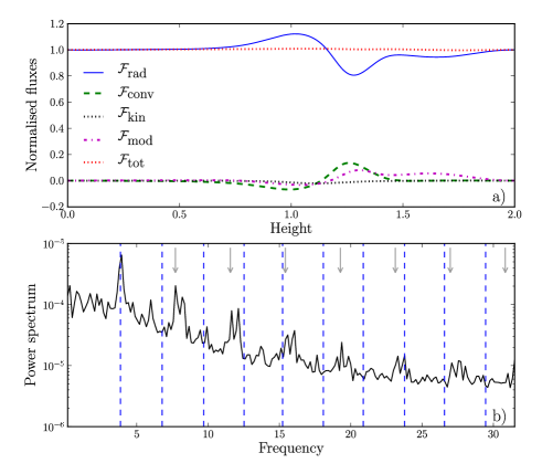
Figure 1: a) Mean vertical profiles of radiative ${\cal F}_{\text{rad}}$ (solid blue line), turbulent enthalpy ${\cal F}_{\text{conv}}$ (dashed green line), kinetic ${\cal F}_{\text{kin}}$ (dotted black line), modes ${\cal F}_{\text{mod}}$ (dot-dashed magenta line) and total ${\cal F}_{\text{tot}}$ (dotted red line) fluxes, normalised to the bottom flux $F_{\hbox{\scriptsize bot}}$. b) Temporal power spectrum for the convective flux only.

The imposed bottom flux $F_{\hbox{\scriptsize bot}}$ is mainly transported through the computational domain by the radiative ${\cal F}_{\text{rad}}$, enthalpy and kinetic ${\cal F}_{\text{kin}}$ fluxes. Following GD2011, the enthalpy flux is divided into the classical convective flux ${\cal F}_{\text{conv}}$ and the contribution coming from the (unstable) fundamental mode (hereafter ${\cal F}_{\text{mod}}$) with

$$\left\{\begin{array}[]{lll}{\cal F}_{\text{conv}}(z,t)&=c_{p}\left\langle\rho u_{z}T^{\prime}\right\rangle,&{\cal F}_{\text{mod}}(z,t)=c_{p}\left\langle\rho u_{z}\right\rangle\theta,\\ \\ {\cal F}_{\text{rad}}(z,t)&=-\left\langle K(T)\nabla T\right\rangle,&{\cal F}_{\text{kin}}(z,t)=\dfrac{1}{2}\left\langle\rho u_{z}u^{2}\right\rangle,\end{array}\right.$$ (3)

where the primed quantities denote the fluctuations about the horizontal average and $\theta$ is the temperature eigenfunction of the fundamental mode. The resulting time-averaged and normalised fluxes are given in Fig. 1a.

The bulk of the total flux is transported by the radiative flux, except in the convective zone where ${\cal F}_{\text{conv}}/F_{\hbox{\scriptsize bot}}\simeq 20\%$, while the kinetic flux is negligible (${\cal F}_{\text{kin}}/F_{\hbox{\scriptsize bot}}\leq 1\%$). Concerning ${\cal F}_{\text{mod}}$, one notes that it is hardly as large as ${\cal F}_{\text{conv}}$ in the convective zone. This quantity is a good signature of the amplitude of the acoustic modes as the higher ${\cal F}_{\text{mod}}$, the larger the radial oscillations (GD2011), therefore confirming the efficiency of the $\kappa$-mechanism in this simulation.

The signature of the temporal modulation of the convective flux is extracted from its Fourier spectrum in time, that is, we first compute $\widehat{\cal F}_{\text{conv}}(z,\omega)$, with $\omega$ the frequency, and second integrate over the vertical direction $z$ to get the power spectrum $\widehat{\cal F}_{\text{conv}}(\omega)$ (Fig. 1b). Several discrete peaks appear about given frequencies, of which the physical nature is emphasised after superimposing the linear acoustic eigenfrequencies (the vertical dashed blue lines). The matching with the fundamental mode frequency $\omega_{00}=3.85$ is perfect while the weak-amplitude secondary peaks rather correspond to harmonics of $\omega_{00}$ (i.e. $2\omega_{00},3\omega_{00},\dots$, shaped by downward-directed vertical gray arrows in Fig. 1b) than to the acoustic overtones $\omega_{01},\ \omega_{02},\dots$. It means that the amplitude of the fundamental acoustic mode is large enough to generate several harmonics through a nonlinear cascade and this is again an indication of both the robustness of the $\kappa$-driving and the relevance of this kind of convection-pulsation simulation to check the TDC recipes.

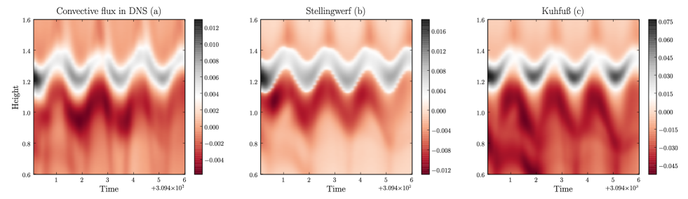
Figure 2: Evolution of the convective flux in a $(t,\ z)$ plane: (a) in the DNS; (b) with Stellingwerf’s formalism ${\cal F}_{\text{St}}$; (c) with Kuhfuß’s formalism ${\cal F}_{\text{Ku}}$ (for $\alpha_{\text{St}}=\alpha_{\text{Ku}}=1$). The vertical extent is centered on both sides of the convection zone to emphasise its oscillations. These snapshots are computed after 1800 periods of oscillations, i.e. well after the nonlinear saturation is achieved.

3.2 DNS vs TDC models: convective patterns

We first compare the time evolution of the horizontally averaged convective flux obtained in the DNS (Eq. 3) with its TDC counterparts ${\cal F}_{\text{St}}$ and ${\cal F}_{\text{Ku}}$ (Eq. 1). As we are interested here in the qualitative agreement between the convective patterns in the plane $(t,\ z)$, we simply assume $\alpha_{\text{St}}=\alpha_{\text{Ku}}=1$.

The three resulting patterns are displayed in Fig. 2 for a time interval spanning about 4 periods of the fundamental acoustic mode. The black areas denote positive values for the convective flux and therefore delimit the convective zone. An oscillatory behaviour is clearly visible in each panel, with a period that looks similar to the one of the fundamental acoustic mode, that is, almost 4 oscillation cycles are depicted. This is consistent with the large peak shown around $\omega_{00}$ in the power spectrum in Fig. 1b.

The two TDC patterns also display a good agreement with the nonlinear simulation regarding the overshooting phenomenon. We indeed recover the same dark red structures below the convective zone that correspond to the downdrafts entering in the radiative zone (this penetration being associated with a negative convective flux). Nevertheless, we note that the overshooting seems to be more vigorous in Kuhfuß’s model than in Stellingwerf’s one as these dark red structures fill in Fig. 2c a larger surface in the bottom radiative zone than in Fig. 2b.

3.3 DNS vs TDC models: statistics of coefficients $\alpha$

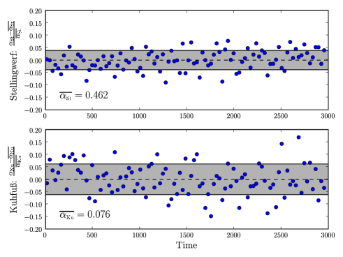
Figure 3: Time evolution around the mean value of coefficients $\alpha_{\text{St}}$ (upper panel) and $\alpha_{\text{Ku}}$ (bottom panel). Horizontal gray spans mark the limits of the associated relative standard deviation.

A one-to-one comparison between the convective flux in the DNS and its TDC predictions requires to find the optimal values of $\alpha_{\text{St}}$ and $\alpha_{\text{Ku}}$. This is done by performing several $\chi^{2}$-tests at different snapshots in the simulation to track the variations of coefficients $\alpha$. The resulting fluctuations of $\alpha_{\text{St}}$ and $\alpha_{\text{Ku}}$ around their mean values are shown in Fig. 3.

The dispersion of the Stellingwerf coefficient $\alpha_{\text{St}}$ (upper panel) is weaker than the Kuhfuß one (lower panel) as its values are almost within a $5\%$ range around the mean $\overline{\alpha_{\text{St}}}=0.462$. On the contrary, several outliers with values greater than $10\%$ are found in the evolution of $\alpha_{\text{Ku}}$ which then appears more chaotic around the mean value $\overline{\alpha_{\text{Ku}}}=0.076$. As a consequence, the relative standard deviation (depicted in gray in Fig. 3) is weaker in Stellingwerf’s case than in Kuhfuß’s one.

3.4 DNS vs TDC models: convective fluxes with optimal $\alpha$’s

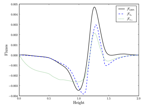
Figure 4: Mean convective flux in the DNS (solid black line), compared with the best TDC predictions based on the optimal $\alpha$ values that came out of the $\chi^{2}$-test in §3.3 (Stellingwerf’s model in dashed blue line and Kuhfuß’s one in dotted green line).

We recall that TDC models assume that the coefficients $\alpha$ entering in Eq. 1 are constant. By adjusting the TDC recipes with the instantaneous convective flux throughout the nonlinear simulation, the optimal value of these coefficients has been deduced. The final test, given in Fig. 4, then consists in the comparison between the mean nonlinear convective flux taken over the entire simulation and its best TDC approximations built from these optimal $\alpha$ values.

This figure emphasises that Stellingwerf’s formulation gives a better agreement than Kuhfuß’s one. Indeed, the Kuhfuß model overestimates the overshooting as the (negative) convective flux remains non-negligible until the bottom of the radiative zone. On the contrary, the Stellingwerf profile better accounts for the local penetration of convective plumes and shows the same exponential-like decay of the negative convective flux when sinking in the radiative zone (e.g. Dintrans 2009). However, the two models are rather similar in the bulk of the convective zone where convection is fully developed. One also notes that they both predict a negative flux at the top of the convective zone, that is, an upper overshooting of convection motions near the surface that is not observed in the nonlinear simulation.

4 Conclusion

The main weakness of theories of time-dependent convection (TDC) lies in the large number of free parameters. This is particularly awkward when convection is strongly coupled with pulsations as, for example, near the red border of the Cepheid instability strip where similar results are obtained with different sets of parameters (Yecko et al. 1998). Additional constraints must be found to reduce the intrinsic degeneracy of models. But the modelling of the interplay between the turbulent convection and oscillations is really a difficult task due to the strong nonlinearities involved in this coupling.

One solution to tackle this problem and to bring new constraints consists in performing fully nonlinear simulations, and this is the path we have chosen in this work following our first study in GD2011. Two widely used TDC theories, namely the Stellingwerf (1982) and Kuhfuß (1986) ones, are compared with results coming from 2-D nonlinear simulations of compressible convection in which strong acoustic oscillations are self-sustained by the $\kappa$-mechanism. The heat transport is then modulated by the fundamental acoustic mode such that this kind of simulation is relevant to investigate the convection-pulsation coupling (Figs. 1-2).

Focusing on the two TDC formulae for the convective flux, we compute the evolution of free coefficients “$\alpha$” from a $\chi^{2}$-test applied to the fully nonlinear results (Fig. 3). A large temporal variability is found in both cases that weakens the robustness of the TDC assumption $\alpha=\hbox{const}$. Moreover, the mean values $\overline{\alpha}$ are not universal. By applying the same method to other simulations performed in GD2011 (Table 1), we indeed do not recover the same $\overline{\alpha}$ with a relative standard deviation of about $12\%$ (Stellingwerf) and $18\%$ (Kuhfuß).

Table 1: Values of the optimal Stellingwerf and Kuhfuß $\alpha$ coefficients pulled out from the nonlinear simulations in GD2011.

Simulation	$\overline{\alpha_{\text{St}}}$	$\overline{\alpha_{\text{Ku}}}$
G8	0.46	0.076
G8H9	0.47	0.099
G8H8	0.33	0.113
G7	0.38	0.098
G6	0.38	0.102
G6F7	0.40	0.082
G6F5	0.38	0.067

Within these limits, Stellingwerf’s formulation is found to give a better agreement with the nonlinear simulations than Kuhfuß’s one: (i) the final mean convective flux ${\cal F}_{\text{St}}$ is closer to its DNS counterpart, with a much better estimation of the bottom overshooting; (ii) the temporal dispersion of the $\alpha_{\text{St}}$ coefficient is weaker, then its enhanced stability (Fig. 4). This result means that the time-dependent convective flux better scales with a law ${\cal F}_{\text{conv}}\propto{\cal E}_{t}\sqrt{\nabla-\nabla_{\text{ad}}}$ than ${\cal F}_{\text{conv}}\propto\sqrt{{\cal E}_{t}}(\nabla-\nabla_{\text{ad}})$, and the Stellingwerf formulation may probably be preferred in the 1-D hydrocode used in, e.g., the topical Cepheids models. However, this study emphasises that both formalisms lead to an artificial overshooting at the top of the convection zone. We also note that this TDC test involves the exact value of the turbulent kinetic energy ${\cal E}_{t}$ provided by the nonlinear simulation, and not by the dedicated 1-D TDC equation which is inherently less accurate. As a consequence, the obtained profiles are certainly the best we can expect from these TDC recipes.

In this work, the temporal modulation of the convective flux is ensured by the acoustic modes excited by $\kappa$-mechanism. An interesting prospect could be the case of a modulation based on the internal gravity waves excited by convection itself. Indeed, convection can excite gravity waves in variable stars, either by the means of the penetration of convective elements into stably stratified regions as in solar-type stars (e.g. Dintrans et al. 2005), or through the so-called “convective blocking” mechanism as in white dwarfs or Gamma Doradus stars (e.g. Pesnell 1987). In both cases, the convective flux is ipso facto modulated by gravity waves and it may be interesting in that respect to also check the accuracy of time-dependent convection models.

Online Material

Appendix A Setup of the simulations

A.1 The equilibrium model

Table 2: Dimensionless parameters of the numerical simulations.

DNS	Gravity $\@vec{g}$	Flux $F_{\hbox{\scriptsize bot}}$	Conductivity $K_{\hbox{\scriptsize max}}$	$T_{\hbox{\scriptsize bump}}$	Width $e$	Slope $\sigma$	Viscosity $\nu$	Frequency $\omega_{00}$	Rayleigh
G8	8	$4.5\times 10^{-2}$	$10^{-2}$	6	1	1	$2.5\times 10^{-4}$	$3.85$	$10^{5}$
G8H9	8	$4.5\times 10^{-2}$	$9\times 10^{-3}$	7	1	1	$5\times 10^{-4}$	$3.83$	$10^{5}$
G8H8	8	$4.5\times 10^{-2}$	$8\times 10^{-3}$	7.5	1	1.1	$5\times 10^{-4}$	$3.80$	$2\times 10^{5}$
G7	7	$4\times 10^{-2}$	$10^{-2}$	5.5	1.5	0.8	$2.5\times 10^{-4}$	$3.62$	$8\times 10^{4}$
G6	6	$4\times 10^{-2}$	$10^{-2}$	6	1.5	0.8	$5\times 10^{-4}$	$3.35$	$8\times 10^{4}$
G6F7	6	$3.7\times 10^{-2}$	$10^{-2}$	5.7	1.5	0.8	$3.5\times 10^{-4}$	$3.36$	$9\times 10^{4}$
G6F5	6	$3.5\times 10^{-2}$	$10^{-2}$	5.5	1.5	0.8	$3\times 10^{-4}$	$3.36$	$9\times 10^{4}$

As in GD2011, our system represents a zoom around an ionisation region. As we are computing local simulations, the vertical gravity $\@vec{g}=-g\@vec{e_{z}}$ and the kinematic viscosity $\nu$ are assumed to be constant. Following our purely radiative model of the $\kappa$-mechanism (Gastine & Dintrans 2008a, b), the ionisation region is represented by a temperature-dependent radiative conductivity profile that mimics an opacity bump:

$$K(T)=K_{\hbox{\scriptsize max}}\left[1+{\cal A}\dfrac{-\pi/2+\arctan(\sigma T^{+}T^{-})}{\pi/2+\arctan(\sigma e^{2})}\right],$$ (4)

with

$${\cal A}=\dfrac{K_{\hbox{\scriptsize max}}-K_{\hbox{\scriptsize min}}}{K_{\hbox{\scriptsize max}}},\quad T^{\pm}=T-T_{\hbox{\scriptsize bump}}\pm e,$$ (5)

where $T_{\hbox{\scriptsize bump}}$ is the position of the hollow in temperature and $\sigma$, $e$, and ${\cal A}$ denote its slope, width, and relative amplitude, respectively. We assume both radiative and hydrostatic equilibria; that is,

$$\left\{\begin{aligned} \dfrac{dp_{0}}{dz}&=-\rho_{0}g,\\ \dfrac{dT_{0}}{dz}&=-\dfrac{F_{\hbox{\scriptsize bot}}}{K_{0}(T_{0})},\\ \end{aligned}\right.$$ (6)

where $F_{\hbox{\scriptsize bot}}$ is the imposed bottom flux. Following GD2011, we chose $L_{z}$ as the length scale, i.e. $[x]=L_{z}$, top density $\rho_{\hbox{\scriptsize top}}$ and top temperature $T_{\hbox{\scriptsize top}}$ as density and temperature scales, respectively. The velocity scale is then $\sqrt{c_{p}T_{\hbox{\scriptsize top}}}$, while time is given in units of $[t]=L_{z}/\sqrt{c_{p}T_{\hbox{\scriptsize top}}}$.

Table 2 then summarises in these dimensionless units the parameters of the numerical simulations presented in this study. The penultimate column of this table contains the value of the frequency $\omega_{00}$ of the fundamental unstable radial mode excited by the $\kappa$-mechanism, which lies between 3 and 4 for every DNS. The last column gives the value of the Rayleigh number, which quantifies the strength of the convective motions. It is given by

$$\text{Ra}=\dfrac{gL_{\text{conv}}^{4}}{\nu\chi c_{p}}\left|\dfrac{ds}{dz}\right|,$$ (7)

where $L_{\text{conv}}$ is the width of the convective zone, $\chi=K_{0}/\rho_{0}c_{p}$ the radiative diffusivity, and $s$ the entropy.

A.2 The nonlinear equations

With the parallel alternate direction implicit solver for the radiative diffusion implemented in the pencil code (see GD2011), we advance the following hydrodynamic equations in time:

$$\left\{\begin{aligned} \displaystyle\frac{D\ln\rho}{Dt}=&-\mathop{\hbox{div}}\nolimits\@vec{u},\\ \\ \displaystyle\frac{D\@vec{u}}{Dt}=&-\dfrac{1}{\rho}\@vec{\nabla}p+\@vec{g}+2\nu\left(\@vec{\nabla}\cdot\@vec{\sf S}+\@vec{\sf S}\cdot\@vec{\nabla}\ln\rho\right),\\ \\ \displaystyle\frac{DT}{Dt}=&\frac{1}{\rho c_{v}}\mathop{\hbox{div}}\nolimits K(T)\@vec{\nabla}T-(\gamma-1)T\mathop{\hbox{div}}\nolimits\@vec{u}+2\rho\nu\@vec{\sf S}^{2},\end{aligned}\right.$$ (8)

where $\rho,\ \@vec{u}$, and $T$ denote density, velocity, and temperature, respectively, while $K(T)$ is given by Eq. 4. The operator $D/Dt=\partial/\partial t+\@vec{u}\cdot\@vec{\nabla}$ is the usual total derivative, while $\@vec{\sf S}$ is the (traceless) rate-of-strain tensor given by

$${\sf S}_{ij}=\frac{1}{2}\left(\frac{\partial u_{i}}{\partial x_{j}}+\frac{\partial u_{j}}{\partial x_{i}}-\frac{2}{3}\delta_{ij}\mathop{\hbox{div}}\nolimits\@vec{u}\right).$$ (9)

Finally, we impose that all fields are periodic in the horizontal direction, while stress-free boundary conditions (i.e. $u_{z}=0$ and $du_{x}/dz=0$) are assumed for the velocity in the vertical one. Concerning the temperature, a perfect conductor at the bottom (i.e. flux imposed) and a perfect insulator at the top (i.e. temperature imposed) are applied.

In order to ensure that both the nonlinear saturation and thermal relaxation are achieved, the simulations were computed over very long times, typically $t\gtrsim 3000$. As the eigenfrequency of the unstable acoustic mode $\omega_{00}\in[3-4]$ (see Table 2), this corresponds approximately to 1800 periods of oscillation.