Planetesimals in Debris Disks of Sun-like Stars

Abstract

Observations of dusty debris disks can be used to test theories of planetesimal coagulation. Planetesimals of sizes up to a couple thousand kms are embedded in these disks and their mutual collisions generate the small dust grains that are observed. The dust luminosities, when combined with information on the dust spatial extent and the system age, can be used to infer initial masses in the planetesimal belts. Carrying out such a procedure for a sample of debris disks around Sun-like stars, we reach the following two conclusions. First, if we assume that colliding planetesimals satisfy a primordial size spectrum of the form $dn/ds\propto s^{-q}$, observed disks strongly favor a value of $q$ between $3.5$ and $4$, while both current theoretical expectations and statistics of Kuiper belt objects favor a somewhat larger value. Second, number densities of planetesimals are two to three orders of magnitude higher in detected disks than in the Kuiper belt, for comparably-sized objects. This is a surprise for the coagulation models. It would require a similar increase in the solid surface density of the primordial disk over that of the Minimum Mass Solar Nebula, which is unreasonable. Both of our conclusions are driven by the need to explain the presence of bright debris disks at a few Gyrs of age.

1. Introduction

Dusty disks made up of rocky and icy debris have been observed around other stars, both in reflected optical light (Smith & Terrile, 1984) and in long wavelength thermal radiation (Aumann et al., 1984). Multiple surveys have reported that a significant fraction of main-sequence stars harbor detectable infrared excesses: $\sim 15\%$ solar-type stars (Trilling et al., 2008; Lawler et al., 2009), and $\sim 30\%$ for A-stars (Su et al., 2006). The infrared luminosity, when compared to the luminosity of the central star, ranges from $\sim 10^{-5}$ to $\sim 10^{-3}$. In contrast, the fractional dust luminosity from the Kuiper belt is estimated to be $\sim 10^{-7}$ (Teplitz et al., 1999) and remains undetected.

The observed excess luminosities arise primarily from small ($\sim\mu m-mm$) dust grains. Due to their short survival time (Artymowicz & Clampin, 1997), these grains are believed to be continuously produced by collisions between large parent bodies (‘planetesimals’). These planetesimals, analogous to the Kuiper belt objects in our own system, are in turn left-overs from the epoch of planet formation.

In this article, we describe how we can use debris disks to test theories of planetesimal formation. We first focus our attention on the primordial size spectrum of planetesimals, often characterized by a single power-law, $dn/ds\propto s^{-q}$, where $s$ is the size. In the following, we briefly summarize theoretical understandings and observational evidences for the value of $q$.

The conventional picture of planetesimal formation is composed of a number of steps. The formation of the first generation planetesimals is not yet well-understood and is an area of active research (see, e. g. Youdin & Shu, 2002; Dominik et al., 2007; Johansen et al., 2007; Garaud, 2007). If these are sufficiently massive, gravity dominates their subsequent growth (Weidenschilling et al., 1997). At first, objects grow in an orderly fashion, where collisions and conglomerations occur at rates that are proportional to their geometric cross sections. But when these bodies become so massive that the effect of gravitational focusing becomes significant, run-away growth commences where the largest bodies accrete small planetesimals at the highest rate and quickly distance themselves from their former peers (Wetherill & Stewart, 1989; Kokubo & Ida, 1996). The run-away phase is succeeded by the oligarchic phase where individual large bodies are responsible for stirring the small bodies that they accrete (Kokubo & Ida, 1995, 1998). At the end of these steps, an entire size spectrum of planetesimals are produced. This is the ‘primordial spectrum’.

During the run-away phase, N-body simulations have typically produced a slope of $q\sim 6$ (Kokubo & Ida, 1996; Morishima et al., 2008). This slope is naturally explained if there is energy equi-partition among planetesimals of different sizes (Makino et al., 1998). Moreover, one expects that the distribution becomes shallower (smaller $q$) if larger planetesimals have higher kinetic energies. This indeed occurs during the oligarchic phase when all small and intermediate-sized planetesimals are stirred to the same velocity dispersion. The value of $q$ is then reduced to $\approx 4$ (Morishima et al., 2008).

Using particles-in-a-box simulations and later hybrid simulations, Kenyon & Luu (1999); Kenyon & Bromley (2004b, 2008) followed the growth of planetesimals. They also found that $q$ decreases with time after the run-away phase, finishing up with $3.75\leq q\leq 4.5$ for planetesimals of sizes between $10$ and $1000$ kms. Recently, Schlichting & Sari (2011) argued analytically that a $q=4$ spectrum is the natural outcome of conglomeration.

Observational constraints on the value of $q$ currently come exclusively from counting large Kuiper belt objects. Kuiper belt objects larger than about $30-50$ kms are commonly believed to be primordial. Collision timescales for these bodies well exceed that of the Solar system age (Davis & Farinella, 1997; Bianco et al., 2010). The size distribution for these bodies can be probed by present-day surveys. Published values for $q$ are scattered: $q=4.0_{-0.6}^{+0.5}$ (Trujillo et al., 2001), $q=4.25\pm 0.25$ (Fraser et al., 2008), $q=4.5\pm 0.4$ (Fraser & Kavelaars, 2009) and $q=4.5_{-0.5}^{+1.0}$ (Fuentes & Holman, 2008). This scatter may be intrinsic and reflect both the different size ranges and the different dynamical populations emphasized by various surveys (Bernstein et al., 2004; Donnison, 2006; Fraser et al., 2010). For bodies smaller than $\sim 30$ kms, the size distribution adopts a shallower power-law (Bernstein et al., 2004; Fuentes & Holman, 2008; Schlichting et al., 2009). This break in the power-law index has been argued to be due to collisional erosion (Pan & Sari, 2005), but a different opinion has surfaced (Charnoz & Morbidelli, 2006).

So at least for the value of $q$, current coagulation models appear to be vindicated by the observations. These models enjoy a further success. In the Kuiper belt region, the solid mass of the so-called Minimum Mass Solar Nebula is $\sim 10~{}M_{\oplus}$ (Hayashi, 1981; Weidenschilling, 1977), while the mass in large Kuiper belt objects is estimated to be $\lesssim 0.1M_{\oplus}$ (see, e.g. Gladman et al., 2001; Bernstein et al., 2004). This large difference, however, is explained by current models where the formation of large planetesimals has a very low efficiency (Bromley & Kenyon, 2006; Schlichting & Sari, 2011).

With these two remarkable concordances, one wonders if debris disks will ever tell us anything new and unexpected. Furthermore, every debris disk likely has a different initial condition and evolves in a different dynamical environment. For instance, dynamical interactions with Neptune or other planets may have qualitatively affected the evolution of the Kuiper belt (Levison et al., 2008). It seems difficult, therefore, to extract any universal truth about the formation process from these disparate objects.

However, based only on a modest sample of debris disks, we argue in this paper that there is already a serious issue in current coagulation models.

To achieve this, we first construct a simple collisional model (§2) to compare against the set of debris disks reported in Hillenbrand et al. (2008). Our collisional model does not differ in essence from previous works (Krivov et al., 2005; Wyatt et al., 2007b; Löhne et al., 2008), but we interpret the observations in a new way. This allows us to measure the value of $q$ as well as the initial masses of planetesimal belts (§4). The latter result challenges the current models of planetesimal formation (5). We summarize in §6.

2. Model: Luminosity Evolution of a Debris Disk

The debris phase commences when eccentricities of the primordial planetesimals are further increased so that they no longer coalesce at encounter, but are instead broken into fragments. In this phase, the smallest primordial planetesimals enter into a collisional cascade first, followed by progressively larger bodies. During the collisional cascade, a primordial body is broken down into smaller and smaller fragments until all its mass ends up in small grains. The small grains may spiral in towards the star due to Poynting-Robertson drag, as happens in the Solar system, or, be ground down by frequent collisions to sizes so small that they are promptly removed by radiation pressure, as happens in bright debris disks (Wyatt, 2005).

2.1. Debris Rings

We model the debris disk as a single, azimuthally smooth ring composed of planetesimals of different sizes. The ring is centered at a semi-major axis $a$ with a full radial width of $\Delta a$ and a constant surface density. We take $\Delta a/a=0.1\ll 1$ as our standard input. This is motivated by the following observations. Spatially resolved debris disks often appear as narrow rings. Examples are, $\Delta a/a$ $\sim 0.1$ for AU Microscopii (Fitzgerald et al., 2007), $\sim 0.5$ for HD 10647 (Liseau et al., 2010), $\sim 0.3$ for HD 92945 (Golimowski et al., 2007), $\sim 0.3$ for HD 139664 (Kalas et al., 2006), $\sim 0.2$ for HD 207129, (Krist et al., 2010), $\sim 0.5$ for $\epsilon$ Eridani (Dent et al., 2000), $\sim 0.1$ for Fomalhaut (Kalas et al., 2005), $\sim 0.2$ for Vega (Su et al., 2005). Similarly, unresolved disks often exhibit spectral energy distribution that is well fit by a single temperature blackbody (Hillenbrand et al., 2008; Nilsson et al., 2010; Moór et al., 2011). This ring-like topology also show up in our own Solar system, hence the name the asteroid “belt” and the Kuiper “belt”.

2.2. Initial Size Distribution of the Planetesimals

We adopt the following power-law forms for the initial size distributions,

$$\left.\frac{dn}{ds}\right|_{t=0}\propto\begin{cases}s^{-q_{3}}\quad\quad s_{\rm small}<s<s_{\rm big},\\ s^{-q_{1}}\quad\quad s_{\rm min}<s<s_{\rm small}.\\ \end{cases}$$ (1)

The index $q_{3}$ is the primordial size index for large bodies, like one that arises out of conglomeration models. Previous studies of collisional debris disks have taken this value to be a given, in fact it is commonly set to be the power law one expects from collisional equilibrium (Krivov et al., 2005, 2006; Wyatt et al., 2007b; Löhne et al., 2008). In contrast, in this contribution we use the observed sample to measure this value.

In equation (1), $s_{\rm big}$ is the size of the biggest planetesimals, $s_{\rm min}$ the smallest. The intermediate size $s_{\rm small}$ is introduced for the purpose of mass accounting: the original mass counts only those between $s_{\rm big}$ and $s_{\rm small}$,

$$M_{0}=\int_{s_{\rm small}}^{s_{\rm{big}}}\frac{4\pi}{3}\rho s^{3}\,n_{3}s^{-q_{3}}\,ds.$$ (2)

While $s_{\rm min}$ is naturally taken to be the size at which radiation pressure unbinds dust grains from the star ( $\sim\mu m$ for a Sun-like star), we discuss our choice for $s_{\rm big}$ and $s_{\rm small}$ below.

Motivated by the observational and numerical results discussed in §1, we investigate values of $q_{3}$ between $3.5$ and $5$. The value $q_{3}=4$ has the special property that mass is distributed equally among all logarithmic size ranges, while masses in systems with $q_{3}>4$ diverge toward the small end. The intermediate size $s_{\rm small}$ is introduced, partly to avoid dealing with this divergence. For sizes below $s_{\rm small}$, we assume that collisions have set up an equilibrium power law with index $q_{1}$ (see Appendix). So, the intermediate size $s_{\rm small}$ can also be interpreted as the collisional break size at time zero. For our study, we set $s_{\rm small}=100$ m. For our typical disks, we find that, within a few million years, collisional equilibrium is established for bodies up to sizes $\sim 1$ km. So the choice of $s_{\rm small}$ is not important for late time evolution.

The choice of size for the largest bodies, $s_{\rm big}$, deserves some discussion, as it affects the qualitative character of the evolution. As a collisional cascade progresses, bodies of larger and larger sizes come into collisional equilibrium, opening up fresh mass reserve to produce the small particles. Once the largest bodies enter into collisional equilibrium, the dust production rate decays with time as $L_{\rm IR}\propto t^{-1}$ (Wyatt et al., 2007a). Two previous studies (Wyatt et al., 2007b; Löhne et al., 2008) have adopted sizes for the largest bodies of $s_{\rm big}=30$ and $74$ km, respectively. For some of their disks, the largest bodies can enter collision equilibrium during the lifetime of the system.

Both Kuiper belt observations and numerical studies of coagulation favor a largest size of $\sim 1000$ km. The largest object yet found in the Kuiper Belt, (136199) Eris, has a radius of $1200\pm 50$ km (Brown et al., 2006). In the simulations of Kenyon & Bromley (2004a), coagulation of planetesimals at 30 - 150 AU produces bodies as large as $1000$ - $3000$ km. When the largest bodies reach this size, self-stirring increases the velocity dispersion and collisions become destructive rather than conglomerating.

Therefore, we adopt a maximum body size of $1000$ km in our study. Our quoted masses reflect this choice of $s_{\rm big}$. Our largest bodies never enter into collisional equilibrium. If this assumption turns out to be erroneous, namely, $s_{\rm big}$ is much smaller and enters into collisional cascade within system lifetime, our model would underestimate the initial masses for old disks. As a result, we would overestimate the value for $q_{3}$.

2.3. Collisions

We only consider collisions that are catastrophically destructive. A catastrophic collision is defined as one that removes at least $50\%$ of the mass of the primary body. In so doing, we have implicitly assumed that both cratering collisions and conglomerating collisions are unimportant. When a destructive collision occurs, the total mass (bullet plus target) is redistributed to all smaller sizes according to $dn/ds\propto s^{-4}$. This choice is somewhat arbitrary and we have confirmed that modifying it (within reasonable bounds) does not change our results.

We do not model evolution of the orbital dynamics as bodies collide. This is justified by the discussions in §5.2.

Let the chance of collisions between two bodies of sizes $s$ and $s^{\prime}$ be,

$$f_{\rm{collision}}=\frac{\pi\left(s+s^{\prime}\right)^{2}}{2\pi a\Delta a\,t_{\rm{orb}}},$$ (3)

Here, $2\pi a\Delta a$ is the surface area spanned by the debris ring in the orbital plane, and $t_{\rm orb}$ is the orbital period. Gravitational focusing is negligible for the high random velocities we consider here. The typical encounter velocity, for particles with eccentricity $e$ and inclination $i$, is (Wetherill & Stewart, 1993)

$$v_{\rm{col}}=\sqrt{1.25e^{2}+i^{2}}\,v_{\rm{kep}},$$ (4)

where $v_{\rm kep}$ is the local Keplerian velocity. We adopt $i\approx e/2$ so $v_{\rm col}\approx 1.32\,e\,v_{\rm kep}$. As argued in §5.2, it is reasonable to assume a constant eccentricity (and inclination) for all bodies. We take a value of $e=0.1$ as the standard input, and discuss this assumption in §5.

We denote the specific impact energy required to catastrophically disrupt a body (target) as ${Q}^{*}$. The scaling of $Q^{*}$ with the size of the target depends on whether its strength is dominated by material cohesion or self-gravity. We adopt the following form (Benz & Asphaug, 1999),

$${Q}^{*}~{}=~{}A\left(\frac{s}{1~{}\mbox{cm}}\right)^{\alpha}+B\rho\left(\frac{s}{1~{}\mbox{cm}}\right)^{\beta}$$ (5)

where $\rho$ is the bulk density which we take to be $2.5\rm{g}/\,\rm cm^{3}$. The first term on the right-hand-side describes the internal strength limit, important for small bodies, while the second term the self-gravity limit, important for larger bodies.

The strength law sets the size of the smallest bullets required to destroy a target. Since these are also the most numerous, they determine the downward conversion rate of mass during a collisional cascade. As such, the power indexes in the strength law directly determine the size spectrum at collisional equilibrium. For a strength law of the form ${Q}^{*}\propto s^{c}$, the equilibrium size spectrum is $dn/ds\propto s^{-q}$, with (Durda & Dermott, 1997):

$$q=(21+c)/(6+c).$$ (6)

The famous Dohnanyi-law (Dohnanyi, 1969), $dn/ds\propto s^{-3.5}$, obtains from $c=0$.

The value and form for $Q^{*}$ are notoriously difficult to assess. It depends on, among other factors, material composition, porosity and impact velocity. A number of computations and compilations have appeared in the literature. We select three representative formulations for our study (Fig. 1).

Based on a variety of experimental data and SPH simulations, Krivov et al. (2005); Löhne et al. (2008) advocated the following choices, $A=2\times 10^{7}\,\rm erg/\rm g$, $\alpha=-0.3$, $B=0.158$, $\beta=1.5$. We call this the ’hard’ strength law. In this case, the collision spectrum satisfies $q\approx 3.6$ and $3.0$, in the strength and gravity regimes respectively.

Based on energy conservation, Pan & Sari (2005) calculated a destruction threshold for bodies that have zero internal strength and obtained $B=3.3\times 10^{-8}$, $\beta=2$. So bodies at $100\,\rm km$ is weaker by a factor $\sim 1000$ than their counterparts in the Krivov et al. (2005) formulation. We refer to this as the ’soft’ strength law. A softer strength implies smaller bullets and therefore more frequent destruction of the targets. Pan & Sari (2005) did not consider smaller bodies that are strength bound. We adopt $A=2\times 10^{7}\,\rm erg/g$ and $\alpha=-0.3$ in this range to complete the soft prescription.

Stewart & Leinhardt (2009) proposed a strength law that depends on impact velocity,

$$Q^{*}=\left(500\,s^{-0.33}+10^{-4}\,s^{1.2}\right)v_{\rm col}^{0.8},$$ (7)

For a typical velocity $v_{\rm col}=500$m/s and for bodies greater than 1km, this gives rise to a strength law that falls in-between that of the hard and the soft case. We call this the medium strength law. Note that this strength law is much weaker than the other two for small bodies.

For the strength laws we consider, transitions from material strength domination to self-gravity domination occur at size $s\approx s_{1}$, with $s_{1}$ ranging between $100$ m (the hard and the medium laws) and $10$ km (the soft law).

Figure 1.— Prescriptions for specific strength from Löhne et al. (2008), Pan & Sari (2005) and Stewart & Leinhardt (2009), plotted here as functions of target sizes. We insert an impact velocity of $500\,\rm m/\,\rm s$ to evaluate the last prescription. Strength of small bodies are dominated by material cohesion, while that of larger bodies by self-gravity. Transitions between the two limits occur around $100$ m (the hard and the medium laws) or around $10$ km (the soft law). Strength for bodies smaller than $1\,\rm cm$ are extrapolations as both laboratory and numerical experiments only concern bodies of larger sizes.

2.4. Luminosity Evolution

Figure 2.— Time evolution of the break-size in a model system, with $M_{0}=12.4M_{\oplus}$, $q_{3}=4.0$, $e=0.1$, $a=31\rm{AU}$, and $\Delta a/a=0.1$. Here, break-size is defined as the size at which all bodies initially at that size have encountered of order one destructive collision. Break size increases with time monotonically as larger bodies enter into collisional cascade. The numerical results are shown as solid curves, while the analytical scaling relations (see Appendix) are plotted as dashed lines. The bends in the curves occur at $s\approx s_{1}$, i.e., sizes for which material cohesion and gravity binding are comparable. The set of thick curves are for the case of hard material strength, while the thin lines for soft strength.

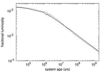
Figure 3.— Evolution of fractional luminosity, $L_{\rm IR}/L_{*}$, for the system in Fig. 2. The thick line is obtained using the hard strength law, and the thin line the soft one. The evolution proceeds in two stages: the flatter early stage when collisional cascade only involves small bodies that are bound by material cohesion; and a steeper later stage where bodies bound by self-gravity enter the cascade. At late times, fractional luminosity decays as $t^{-0.5}$ (eq. (A9)). While break-sizes differ for the two adopted strength laws (Fig. 2), this appears to have little influence on the overall luminosity.

The planetesimal disk, starting from an initial disk mass of $M_{0}$, and an initial size spectrum (eq. 1), is numerically collided and ground down. We divide the particles between $s_{\rm small}$ and $s_{\rm big}$ into $500$ equal logarithmic size bins. The time-step for the simulations is adaptively set so that over one time-step, the maximum mass gain (from larger bodies) or loss (to smaller bodies) per bin falls below $5\%$. The net mass change is substantially smaller than this due to the cancellation between gain and loss.

We calculate the fractional brightness of the dust disk, $L_{IR}/L_{*}$, by integrating the geometrical cross section over all grains. This assumes that grains are perfect absorbers at the optical and can emit efficiently in the infrared.

An example of such a calculation is reported in Figs. 2 & 3. To understand these results, a simple analytical model (see Appendix) is introduced. Scaling relations obtained using this analytical model compares well with our numerical results.

Fig. 2 shows that, with time, larger and larger planetesimals enter into collisional cascade. Within a million years or so, the cascade has advanced to size of order one kilometer. Beyond this time, bodies bound by self-gravity can be gradually eroded. By 1 Gyrs, bodies with sizes $10-100$ kms may be affected. The exact value depends on the strength law. The dust luminosity is related to the dust mass, which is in turn related to the dust production rate. The dust production rate, on the other hand, is simply the primordial mass stored at the break-size divided by the system age. If the primordial spectrum is such that a large amount of mass is piled at the large end, debris disks would not exhibit significant fading even up to a few billion years.

Fig. 3 shows that dust luminosity $L_{\rm IR}/L_{*}\propto t^{-0.5}$ for $q_{3}=4$, consistent with equation (A11). That same equation also demonstrates that the value of $B$, strength constant for bodies bound by self-gravity, affects the luminosity only minorly. This is born out by results shown in Fig. 3.

An important result on which we base our later analysis is shown in Fig. 4. Luminosity evolution for disks with the same initial mass but different $q_{3}$ are depicted. As eq. (A9) predicts, $L\propto t^{(q_{3}-3)/(2-q_{3})}$. If $q_{3}$ is shallow (e.g. $q_{3}\leq 4$), most of the initial mass is deposited at the largest planetesimals. This mass reservoir is harder to reach by collision and allows the disk to remain brighter at later times. In comparison, disks with a steeper $q_{3}$ decay faster.

If one observes a collection of debris disk all at the same age, intrinsic scatter in, e.g., initial masses, makes it impossible to differentiate between models of different $q_{3}$. However, a collection of disks with a large age spread can be used to constrain $q_{3}$. This we proceed to demonstrate.

Figure 4.— Luminosity evolution for disks with different $q_{3}$ but the same initial mass ($8M_{\oplus}$). Systems with a steeper primordial size spectrum (larger $q_{3}$) exhibit a more pronounced decline of luminosity with time, since at a given time, a bigger fraction of their mass reservoir has been depleted. Systems with shallower $q_{3}$ (e.g., $q_{3}=3.5$), on the other hand, are initially dimmer due to the relative shortage of smaller rocks, but eventually outshine the higher $q_{3}$ disks as they can hold on to their mass reservoir for longer. The luminosity decay of observed disks that span a large range of ages can thus be used to infer the value of $q_{3}$. All other parameters here are similar to those used in Fig. 3 and we adopt the hard strength law.

3. Observed Ensemble

Several debris disks surveys have been carried out (see, e.g. Su et al., 2006; Trilling et al., 2008; Lawler et al., 2009; Moór et al., 2011). The sample of most interest to us is that reported in Hillenbrand et al. (2008). Together with updates in Carpenter et al. (2009), Hillenbrand et al. (2008) presented a collection of debris disks around F/G/K type stars, obtained as part of the Spitzer program on Formation and Evolution of Planetary Systems (FEPS). This sample is unique in that both the stellar age and the radial distance of the dust ring are determined: isochrone fitting provides the age for the host stars (spanning from $\sim 10^{7}$ years to a few $10^{9}$ years), while multi-band photometry and spectral energy fitting yield the semi-major axis of the dust ring. Together with fractional luminosity of the dust belt, these provide the most important constraints to infer the primordial properties of parent planetesimals.

To obtain the blow-out size ($s_{\rm min}$) for each system, we take luminosity values for the central stars as given in (Hillenbrand et al., 2008), and we assign stellar masses by assuming that $M_{*}\propto L_{*}^{1/3}$, as appropriate for solar type main-sequence stars.

Out of the $31$ disks listed in Hillenbrand et al. (2008), we focus only on a sub-sample of 13 disks that appear radially unextended and are around main-sequence stars. In Hillenbrand et al. (2008), emission from each disk is initially fitted with a single temperature blackbody (a ring). If agreement between the ${24\mu\rm{m}}/{33\mu\rm{m}}$ fit and the ${33\mu\rm{m}}/{70\mu\rm{m}}$ fit is poor, they argue that the disk is likely radially extended and fit the data instead with two radial components. Since our numerical model is a one-zone model, we find that including the extended sources into our analysis causes significant scatter in the results. This leads us to discard them for the current analysis. We have excluded HD 191089 from our sample. Its fluxes in 13 $\mu$m and 33 $\mu$m are not measured, and cannot be reliably identified as an unextended source. In all, we are left with 13 sources.

It is interesting to note that most of the extended sources are relatively young, all younger than a few hundred million years. In contrast, the unextended sources have a larger age spread, lasting till a few billion years (Fig. 5). All systems may be born with more than one debris rings, but after a sufficiently long time, only the outermost ring, which has the longest erosion timescale, remains shining. The extended system are also brighter than the average, likely related to their relative youth.

Figure 5.— Cumulative distribution of stellar age (left panel) and dust luminosity (right panel) for the Hillenbrand et al. (2008) sample. The extended systems (solid curve) tend to be younger and brighter than the unextended systems (dashed curves).

Figure 6.— Inferred disk initial masses, plotted against system ages, for the unextended systems in Hillenbrand et al. (2008). The four panels present four different choices of $q_{3}$. The other parameters chosen are $e=0.1$, $s_{\rm small}=10^{4}\rm{cm}$, and $\Delta a/a=0.1$. A value of $q_{3}\in[3.5,4.0]$ is preferred: the upper envelopes for the disk mass remain constant at all ages in the two top plots. Models with higher $q_{3}$ are excluded as they require a rising upper envelope. In addition, the $q_{3}=5$ model requires unphysically large disk masses for very old disks.

Figure 7.— Similar to Fig. 6 except $q_{3}$ is fixed at $4$ and a number of parameters are varied to test how the inferred initial masses depend on them. Specific values for the inferred mass may change, when the small end of the primordial size spectrum ($s_{\rm small}$, top-left), the eccentricity of particles (bottom-left), the fractional width of the debris ring (top-right), and the adopted strength law (bottom-right) are varied for all systems. However, the important indicator for our study, the upper envelope of the masses as a function of system age, remains flat. So the conclusion that $q_{3}\sim 4$ remains valid.

4. The Primordial Size Spectrum Revealed

We have a simple strategy. Knowing the luminosity, the age and the semi-major axis of each debris ring, we use our collisional model to backtrack the evolution to infer its initial mass in the planetesimal belt. These initial masses, when plotted against system ages, should show a spread. One expects this spread to be constant across all ages, as disks formed at different cosmic times likely have the same distribution of disk properties. This property could be used to test model assumptions. However, using the spread is difficult due to selection effects. For instance, low mass disks may become too dim at late times to be observable. So we propose instead to study the upper envelope of this spread. The upper envelope should be flat with age for the correct model. From our analytical scaling relations (see Appendix), we find that the most important parameter in our model that affects this mass slope is $q_{3}$, the power-law index in the primordial size spectrum.

The results of such a procedure are shown in Fig. 6. Models with $q_{3}=4.5$ or greater appear to be excluded by data, as they would require a rise of initial disk mass with stellar ages. The reason behind this is transparent by studying Fig. 4. Models with $q_{3}=3.5$ and $4$ are compatible with observations. Models with smaller $q_{3}$ lead to a decreasing initial mass with system age and are excluded as well.

Our model employs a number of other parameters, such as the radial position and extent of the debris ring, the dynamical excitation and break-up strength of the particles. We have studied the robustness of our results when these parameters are varied (Fig. 7). As long as the values for these parameters remain constant over age, varying them do not affect our conclusion on $q_{3}$. The assumption that the dynamical excitation is constant over age is suspicious, in light of results from coagulation models showing that stirring by large plantesemals increases gradually eccentricities of the disk particles. This is discussed in §5.

There is significant uncertainty in our conclusion due to the small sample size. However, we argue that a larger sample may still not favor models with, e.g., $q_{3}=5$. If $q_{3}=5$ (lower-right panel in Fig. 4), the system that remains easily detectable at 2 Gyrs of age requires an initial solid mass of $\sim 200M_{\oplus}\sim 1M_{J}$ in the planetesimal belt. The initial gas mass in such a belt will be higher than the total disk mass of a typical T-Tauri star ($0.01M_{\odot}$).

By focusing on dust luminosities, we are sensitive only to bodies that lie below the break-size. As seen in Fig. 2, break-size marches up to few tens to a hundred kilometers by the end of a few billion years, if the disk has a mass of $M_{0}=12.4M_{\oplus}$.

5. Discussions

5.1. Coagulation Models vs. Debris Disks

Figure 8.— Inferred initial masses for a broken power-law size-distribution. We investigate two particular forms, motivated by coagulation simulations by Kenyon & Bromley (2008) and Schlichting & Sari (2011), respectively. Other parameters adopted are $e=0.1$, $\Delta a/a=0.1$, and the hard strength law. The inferred disk mass rises sharply with system age. Moreover, to make old and bright systems, we require disk masses that approach the mass of Jupiter.

In our exercise, we have assumed a simple initial size distribution (eq. 1), with all bodies larger than a few hundred meters described by a single power law index $q_{3}$. We relax this assumption here.

Simulations of planetesimal coagulation produce typically more complicated size distributions. For example, Kenyon & Bromley (2008) started their simulations with all bodies at $\leq 1$ km. After tens of millions of years of growth, most of the mass still remains at or below $1$ km, with only $\sim 8\%$ of the mass being accreted into bodies $10$ km or larger, $\sim 6\%$ into bodies $100$ kms or larger, and $\sim 3\%$ into bodies of order $1000$ kms. We use a broken power-law to replicate this kind of primordial spectrum. We set $q_{3}=5.5$ from $1$ km to $10$ km, and $q_{3}=4$ from $10$ km to $1000$ km. Motivated by Schlichting & Sari (2011), we also consider a slightly different initial distribution with $q_{3}=7$ from $1$ km to $10$ km, and $q_{3}=4$ from $10$ km to $1000$ km. Both sets of size spectrum deposit mass mostly at the low end ($\leq 1$ km) and little at the large sizes. As expected, when initial masses are determined for different systems (Fig. 8), we find that young systems require exceedingly low initial masses, while old systems require unphysically large initial masses.

If we follow the luminosity evolution of such a disk, we will see that the disk flares brightly in the first tens of millions of years, due to the large mass reservoir at the $1$ km-range. Then the luminosity decays as $t^{-1/2}$ (as expected of a $q_{3}=4$ spectrum) but with a low normalization – most of the disk mass has been ground down in the early stage and we are now left with but a scrap remnant of the original. Conglomeration simulations typically find that only a small fraction of the mass can be accreted to make large bodies, before viscous stirring effectively stalls the growth. Schlichting & Sari (2011) showed that the fraction in large bodies can only be of order $10^{-3}$ in Kuiper-belt-like environments.

Does results in Fig. 8 allow us to exclude current conglomeration models? One possible caveat in our analysis is the eccentricity. We discuss this below.

5.2. Eccentricity

We assume a static, high eccentricity ($e=0.1$) for all systems at all times. In realistic systems, eccentricities can be a function of time.

One possible cause of eccentricity evolution is collisional cooling.

Collisions dissipate energy, so collisional products have in average lower velocity dispersion than their parent bodies. In a single collision, two bodies with masses $m_{1}$ and $m_{1}^{\prime}$ (assume $m_{1}\gg m_{1}^{\prime}$) impact with typical velocities

$$v_{1}\sim v_{1}^{\prime}\sim e_{1}\,v_{\rm{kep}},$$ (8)

where the subscript $1$ indicates that this is a first generation collision in our counting. Assuming that all collision debris fly away from the collision site with the velocity of the center-of-mass, i.e., all relative velocities in the center-of-mass frame is dissipated during the collision, collisional cooling can be expressed as

$$v_{2}\sim\frac{\sqrt{m_{1}^{2}v_{1}^{2}+m_{1}^{\prime 2}v_{1}^{\prime 2}}}{m_{1}+m_{1}^{\prime}}\sim v_{1}\left(1-\frac{m_{1}^{\prime}}{2m_{1}}\right).$$ (9)

So the closer in mass the two colliding bodies are, the more cooling their debris experiences. If cooling dominates the eccentricity evolution, we find that a minimum eccentricity of $e_{1}=0.13$ is required (for the hard strength law, and $e_{1}=0.02$ for the medium law) to allow collisional cascade to proceed all the way to micron range.

However, even if collisional cooling is severe, we argue that viscous stirring by large planetesimals dominates the eccentricity evolution. This is able to raise the eccentricity of collisional debris to values comparable to that of their parents in a time shorter than a collisional time. So the condition for a successful collisional cascade is reduced to $e\geq 0.05$ for the hard strength law and $e\geq 0.01$ for the medium strength law, i.e., the minimum random motion necessary to break up the hardest grains (the smallest ones).

In fact, stirring is likely to gradually raise the eccentricity of all bodies. Stirring by large bodies in the disk goes as $e\propto t^{1/4}$ (c.f. Goldreich et al., 2004). In the simulations of Kenyon & Bromley (2008), planetesimals are continuously stirred by Pluto-like bodies, but they only reach $e\sim 0.1$ at about a Gyrs. Under such a scenario, the inferred initial disk mass is similar to the original result (Fig. 9), but it is clear that we prefer the same range of values for $q_{3}$.

Figure 9.— Same as the top-right panel in Fig. 6 but instead of a constant eccentricity ($e=0.1$), here we assume that the eccentricity rises as $e(t)\approx 0.1(t/10^{9}\rm{yrs})^{1/4}$. There is little difference to the inferred mass, and if anything, the data seems to argue that a $q_{3}=4$ model slightly overestimate the value of $q_{3}$. So our conclusion that $q_{3}\in[3.5,4]$ remains unchanged even considering eccentricity growth.

6. Summary

Using an ensemble of bright debris disks around Sun-like stars, we have measured the size spectrum of their embedded planetesimals. We parametrize the size spectrum as $dn/ds\propto s^{-q_{3}}$ and find $q_{3}\approx 3.5-4$, where $q_{3}=4$ corresponds to equal mass per logarithmic decade. The planetesimal sizes our technique probes lie between a couple kms to $\sim 100\,\rm km$.

While this size spectrum appears consistent with results of coagulation simulations ($q_{3}\sim 4$), there are two lines of evidences that suggest problems in current coagulation models.

The first line of evidence is related to the inferre disk mass. The inferred initial masses for these bright disks are surprisingly high. We find total masses reaching as high as $10M_{\oplus}$. This is comparable to the total solid mass in the Kuiper belt region of Minimum Mass Solar Nebula model, and about a factor of $100$ higher than the mass in large Kuiper belt objects. Current coagulation models require an MMSN-like total mass to produce the observed density of large Kuiper belt objects. If the same inefficiency persists for our disks, one would require a total disk mass of $\sim 100$ MMSN to produce those embedded planetesimals. This is difficult to imagine.

The second line of evidence regards the size spectrum. We experiment with size distributions that arise from coagulation simulations. We find that these distributions could not reproduce the luminosity distribution of the observed disks. Current coagulation models are highly inefficient in making large planetesimals. So most of the mass remains at where they started, presumably $\sim 1$ km. This leads to debris disks that are too bright at early times and that are too dim at late times, by a couple orders of magnitude.

We do not believe these discrepancies can be resolved by relaxing some of our model assumptions. In particular, we argue that our estimate for $q_{3}$ is unchanged even taking into account the fact that disk eccentricity may rise with time. Our results are also insensitive to the width of the debris ring, to the strength of bodies, and to the assumed upper and lower sizes.

Because we restrict our attention to the upper envelope of inferred masses, our result is dominated by a handful of systems. Our analysis may be vulnerable to errors. However, the evidence is solid that debris disks remain fairly bright even at a few billion years. This alone dictates that there ought to be lots of mass stored in large (10-100 kms) planetesimals. We address how this is accomplished by revisiting coagulation model in an upcoming publication.

Appendix A Evolution of Debris Disk Properties: Analytical Model

In the following, we present a simple analytical model that describes the time evolution of dust luminosity and size distribution in debris disks. This model is very similar to that described in Löhne et al. (2008), except for our choice for the size of the largest planetesimals. In the following, we present results with arbitrary strength law and initial size distribution, followed by numerical evaluations using the hard strength law and for $q_{3}=4$.

We approximate the body strength (eq. 5) by two broken power-laws,

$$\bar{Q}_{D}=\begin{cases}A\left(\frac{s}{1\rm{cm}}\right)^{\alpha}&\quad s<s_{1}\\ B\rho\left(\frac{s}{1\rm{cm}}\right)^{\beta}&\quad s>s_{1}\\ \end{cases}$$ (A1)

where $s_{1}$ is the size at which the two expressions meet. The body strength is dominated by material strength below $s_{1}$ and by self-gravity above $s_{1}$. For the hard strength law that we adopt, $\alpha=-0.3,\beta=1.5$ and $s_{1}=\left(\frac{B}{A}\rho\right)^{\frac{1}{\alpha-\beta}}\rm{cm}\approx 300$ meters.

Combined with equation (4), the minimum size of an impactor that causes catastrophic disruption is

$$s_{\rm{impactor}}=\begin{cases}\left(\frac{2A}{1.75e^{2}v_{\rm{kep}}^{2}}\right)^{\frac{1}{3}}\left(\frac{s}{\mbox{1 cm}}\right)^{1+\frac{\alpha}{3}}=k_{1}s^{\kappa_{1}}&\quad s<s_{1}\\ \left(\frac{2B\rho}{1.75e^{2}v_{\rm{kep}}^{2}}\right)^{\frac{1}{3}}\left(\frac{s}{\mbox{1 cm}}\right)^{1+\frac{\beta}{3}}=k_{2}s^{\kappa_{2}}&\quad s>s_{1}\\ \end{cases}$$ (A2)

Here, $\kappa_{1}=0.9$ and $\kappa_{2}=1.5$ for our adopted strength law.

We define a break-size, $s_{2}=s_{2}(t)$, to be the size at which the time-integrated chance of destruction per body is unity, or the optical depth for size $s_{2}$ to be hit is,

$$\tau(s_{2})={{t_{\rm orb}}\over{t}}.$$ (A3)

Bodies larger than $s_{2}$ have hardly collided and they retain their primordial size distribution, while bodies smaller than $s_{2}$ have collided many times, and they satisfy the size distribution for collisional equilibrium. If $s_{2}>s_{1}$, we adopt a size distribution that is piece-wise continuous,

$$\frac{dn}{ds}=\begin{cases}n_{1}s^{-q_{1}}=n_{3}s_{1}^{q_{1}-q_{2}}s_{2}^{q_{2}-q_{3}}s^{-q_{1}}&\quad s<s_{1}\\ n_{2}s^{-q_{2}}=n_{3}s_{2}^{q_{2}-q_{3}}s^{-q_{2}}&\quad s_{1}<s<s_{2}\\ n_{3}s^{-q_{3}}&\quad s>s_{2}\\ \end{cases}$$ (A4)

where $q_{1}$ and $q_{2}$ are the power indexes at collisional equilibrium. They are $3.5$ (Dohnanyi, 1969) if the size ratio between the impactor and the target is constant. Given equation (6), we have $q_{1}=3.6$ and $q_{2}=3.0$ for the hard strength law. This piece-wise size distribution breaks down near the blow-out size due to an abrupt deficit of small bullets. A more accurate derivation for the size distribution can be obtained by assuming that the mass loss rate is constant with size, as is carried out in Strubbe & Chiang (2006). The size distribution shows a flare-up toward the blow-out size, and the magnitude of the flare-up depends on, among other things, the value of eccentricity. Our analytical results obtained based on equation (A4) should be regarded as illustrative.

We first obtain the evolution of $s_{2}$ with time. When $s_{2}<s_{1}$, i.e., collisions involve only bodies bound by the material strength, optical depth for destruction at $s_{2}$ is determined by integrating over all its possible bullets,

$$\tau(s_{2})=\frac{n_{3}s_{2}^{q_{1}-q_{3}}}{2\pi a\Delta a}\int_{k_{1}s_{2}^{\kappa_{1}}}^{s_{2}}\,\pi\left(s_{2}+s\right)^{2}s^{-q_{1}}ds=\frac{n_{3}}{2a\Delta a}\frac{1}{q_{1}-1}k_{1}^{1-q_{1}}s_{2}^{q_{1}-q_{3}+2+\kappa_{1}-\kappa_{1}q_{1}}.$$ (A5)

Substituting this into the definition for $s_{2}$ (eq. A3), we obtain

$$s_{2}\propto t^{1\over{-q_{1}+q_{3}-2-\kappa_{1}+\kappa_{1}q_{1}}}$$ (A6)

This yields $s_{2}\propto t^{1.4}$ for our parameters.

Once $s_{2}>s_{1}$, we perform the same exercise and obtain,

$$s_{2}\propto t^{1\over{-q_{2}+q_{3}-2-\kappa_{2}+\kappa_{2}q_{2}}}$$ (A7)

or $s_{2}\propto t^{0.5}$ for our parameters. So at early times, the break size rises steeply with time, due to an abundance of small bullets; while at late times, the break size rises with time more gradually due to the relative paucity of bullets. These two scaling relations are observed in our numerical results (Figure 2).

Now we proceed to derive the scaling of disk luminosity with system age. We let the infrared luminosity to be that portion of the starlight that is intercepted by debris particles. This is directly related to the total surface area of all particles, which is mostly contributed by particles around $s_{\rm min}$. The fractional luminosity is therefore,

$$\frac{L_{\rm{IR}}}{L_{*}}\approx{{\int_{s_{\rm min}}^{s_{2}}\pi s^{2}\,n_{1}s^{-q_{1}}ds}\over{4\pi a^{2}}}\approx\begin{cases}\frac{n_{3}}{4a^{2}(q_{1}-3)}s_{2}^{q_{1}-q_{3}}{s_{\rm{min}}^{3-q_{1}}}\quad\quad\quad\quad s_{2}<s_{1}\\ \frac{n_{3}}{4a^{2}(q_{1}-3)}s_{1}^{q_{1}-q_{2}}s_{2}^{q_{2}-q_{3}}{s_{\rm{min}}^{3-q_{1}}}\quad\quad s_{2}>s_{1}\\ \end{cases}$$ (A8)

So the evolution of luminosity is dictated by the evolution of $s_{2}$ with time. In particular, at late times (when $s_{2}>s_{1}$), the fractional luminosity decays with time gradually,

$$\frac{L_{\rm{IR}}}{L_{*}}\propto s_{2}^{q_{2}-q_{3}}\propto t^{{q_{2}-q_{3}}\over{q_{2}-q_{3}+2+\kappa_{2}-\kappa_{2}q_{2}}}.$$ (A9)

Again, for our choice of parameters, $L_{\rm IR}/L_{*}\propto t^{-0.5}$. If $q_{3}$ alone is varied, $L_{\rm IR}/L_{*}\propto t^{(q_{3}-3)/(2-q_{3})}$ and scales as $t^{-1/3},t^{-1/2}$ and $t^{-2/3}$ for $q_{3}=3.5,4,$ and $5$ respectively. This forms the basis on which we decipher the primordial distribution of planetesimals.

To understand the dependence of the fractional luminosity on a range of parameters, we return to equations (A8), (A7) and (A5), retaining all the neglected constants and obtaining the following expression,

$$\frac{L_{\rm{IR}}}{L_{*}}\approx\begin{cases}\frac{n_{3}}{4a^{2}(q_{1}-3)}\left[\frac{2a\Delta a}{n_{3}}\left(q_{1}-1\right)\frac{t_{\rm{orb}}}{t}\left(\frac{2A}{1.75e^{2}v_{\rm{kep}}^{2}}\right)^{\frac{1}{3}\left(q_{1}-1\right)}\right]^{\frac{q_{1}-q_{3}}{2+\kappa_{1}-\kappa_{1}q_{1}+q_{1}-q_{3}}}s_{\rm{min}}^{3-q_{1}}\quad\quad\quad\quad\quad\quad s_{2}<s_{1}\\ \frac{n_{3}}{4a^{2}(q_{1}-3)}s_{1}^{q_{1}-q_{2}}\left[\frac{2a\Delta a}{n_{3}}\left(q_{2}-1\right)\frac{t_{\rm{orb}}}{t}\left(\frac{2B\rho}{1.75e^{2}v_{\rm{kep}}^{2}}\right)^{\frac{1}{3}\left(q_{2}-1\right)}\right]^{\frac{q_{2}-q_{3}}{2+q_{2}-q_{3}+\kappa_{2}-\kappa_{2}q_{2}}}s_{\rm{min}}^{3-q_{1}}\quad\quad\quad s_{2}>s_{1}\\ \end{cases}$$ (A10)

Substituting our nominal values for the indexes ($\kappa_{1}=0.9$, $\kappa_{2}=1.5$, $q_{1}=3.6$, $q_{2}=3.0$, $q_{3}=4.0$), we simplify the dependency for luminosity into (for at late times when $s_{2}>s_{1}$),

$${{L_{\rm IR}}\over{L_{*}}}\propto t^{-0.5}M_{0}^{0.5}a^{-3.6}\left(\frac{\Delta a}{a}\right)^{0.5}e^{-\frac{2}{3}}M_{*}^{\frac{5}{6}}B^{\frac{1}{3}}A^{-\frac{5}{6}}s_{\rm{min}}^{-0.6},$$ (A11)

where $M_{0}$ is the total mass of the disk, $a$ its radius, $\Delta a/a$ its fractional width, $e$ the eccentricity of particles, $M_{*}$ the central stellar mass, $s_{\rm min}$ the blow-out size, and $A,B$ the strengths. This relation illuminates how our procedure, using luminosity to infer $M_{0}$, can be affected by various parameters. For example, the actual position of the belt is a piece of essential information, while other values should be known roughly to within a factor of a few to avoid gross mis-estimate.

Equation (A10) can also be used to illustrate the effect of a time-varying eccentricity on our estimate for $q_{3}$. At a given dust luminosity, the inferred initial mass scales with the system age and the eccentricity as

$$M_{0}\propto t^{q_{3}-3}e^{\frac{4}{3}\left(q_{3}-3\right)}.$$ (A12)

Let the plantesimals be stirred with a time-dependence of $e\propto t^{\gamma}$. We define a $\bar{q_{3}}$ as the value of $q_{3}$ one obtains by taking a constant eccentricity (in which case $M_{0}\propto t^{{\bar{q}_{3}}-3}$). The true $q_{3}$ is related to it as

$$q_{3}=3+\left({\bar{q}_{3}}-3\right)\left(1+\frac{4}{3}\gamma\right)^{-1}.$$ (A13)

So for $\gamma=1/4$, ${\bar{q}_{3}}=4$, we get the true $q_{3}=3.75$.

Numerically we find a weaker dependency on $\gamma$. This is related to the afore-mentioned flare-up near the blow-out size. If instead of equation (A4), we make the simplifying assumption that the mass loss rate is the same at blow-out size as at other sizes, but that the micron grains are destroyed by similar grains (as opposed to smaller ones), we find that the dust luminosity is proportional to the total number of blow-out grains, while the mass loss rate is proportional to the square of this number. As a result, we write

$${{L_{\rm IR}}\over{L_{*}}}\propto{\dot{M}}^{1/2}.$$ (A14)

From this, we derive the dependence of dust luminosity on time and on eccentricity that are slightly different from those presented in equations (A9), (A11), (A12) and (A13). For instance, in contrast to equation (A13), the dependence of $q_{3}$ on $\gamma$ is logarithmic.

References

- Artymowicz & Clampin (1997) Artymowicz, P. & Clampin, M. 1997, ApJ, 490, 863
- Aumann et al. (1984) Aumann, H. H., Beichman, C. A., Gillett, F. C., de Jong, T., Houck, J. R., Low, F. J., Neugebauer, G., Walker, R. G., & Wesselius, P. R. 1984, ApJL, 278, L23
- Benz & Asphaug (1999) Benz, W. & Asphaug, E. 1999, Icarus, 142, 5
- Bernstein et al. (2004) Bernstein, G. M., Trilling, D. E., Allen, R. L., Brown, M. E., Holman, M., & Malhotra, R. 2004, AJ, 128, 1364
- Bianco et al. (2010) Bianco, F. B., Zhang, Z., Lehner, M. J., Mondal, S., King, S., Giammarco, J., Holman, M. J., Coehlo, N. K., Wang, J., Alcock, C., Axelrod, T., Byun, Y., Chen, W. P., Cook, K. H., Dave, R., de Pater, I., Kim, D., Lee, T., Lin, H., Lissauer, J. J., Marshall, S. L., Protopapas, P., Rice, J. A., Schwamb, M. E., Wang, S., & Wen, C. 2010, AJ, 139, 1499
- Bromley & Kenyon (2006) Bromley, B. C. & Kenyon, S. J. 2006, AJ, 131, 2737
- Brown et al. (2006) Brown, M. E., Schaller, E. L., Roe, H. G., Rabinowitz, D. L., & Trujillo, C. A. 2006, ApJ, 643, L61
- Carpenter et al. (2009) Carpenter, J. M., Bouwman, J., Mamajek, E. E., Meyer, M. R., Hillenbrand, L. A., Backman, D. E., Henning, T., Hines, D. C., Hollenbach, D., Kim, J. S., Moro-Martin, A., Pascucci, I., Silverstone, M. D., Stauffer, J. R., & Wolf, S. 2009, ApJS, 181, 197
- Charnoz & Morbidelli (2006) Charnoz, S. & Morbidelli, A. 2006, in AAS/Division for Planetary Sciences Meeting Abstracts, 34.04–+
- Davis & Farinella (1997) Davis, D. R. & Farinella, P. 1997, Icarus, 125, 50
- Dent et al. (2000) Dent, W. R. F., Walker, H. J., Holland, W. S., & Greaves, J. S. 2000, MNRAS, 314, 702
- Dohnanyi (1969) Dohnanyi, J. W. 1969, J. Geophys. Res., 74, 2531
- Dominik et al. (2007) Dominik, C., Blum, J., Cuzzi, J. N., & Wurm, G. 2007, in Protostars and Planets V, ed. B. Reipurth, D. Jewitt, & K. Keil, 783–800
- Donnison (2006) Donnison, J. R. 2006, Planet. Space Sci., 54, 243
- Durda & Dermott (1997) Durda, D. D. & Dermott, S. F. 1997, Icarus, 130, 140
- Fitzgerald et al. (2007) Fitzgerald, M. P., Kalas, P. G., Duchêne, G., Pinte, C., & Graham, J. R. 2007, ApJ, 670, 536
- Fraser et al. (2010) Fraser, W. C., Brown, M. E., & Schwamb, M. E. 2010, Icarus, 210, 944
- Fraser & Kavelaars (2009) Fraser, W. C. & Kavelaars, J. J. 2009, AJ, 137, 72
- Fraser et al. (2008) Fraser, W. C., Kavelaars, J. J., Holman, M. J., Pritchet, C. J., Gladman, B. J., Grav, T., Jones, R. L., Macwilliams, J., & Petit, J.-M. 2008, Icarus, 195, 827
- Fuentes & Holman (2008) Fuentes, C. I. & Holman, M. J. 2008, AJ, 136, 83
- Garaud (2007) Garaud, P. 2007, ApJ, 671, 2091
- Gladman et al. (2001) Gladman, B., Kavelaars, J. J., Petit, J., Morbidelli, A., Holman, M. J., & Loredo, T. 2001, AJ, 122, 1051
- Goldreich et al. (2004) Goldreich, P., Lithwick, Y., & Sari, R. 2004, ARA&A, 42, 549
- Golimowski et al. (2007) Golimowski, D., John Krist, J., Chen, C., Stapelfeldt, K., Ardila, D., Clampin, M., Schneider, G., Silverstone, M., Ford, H., & Illingworth, G. 2007, in In the Spirit of Bernard Lyot: The Direct Detection of Planets and Circumstellar Disks in the 21st Century
- Hayashi (1981) Hayashi, C. 1981, Progress of Theoretical Physics Supplement, 70, 35
- Hillenbrand et al. (2008) Hillenbrand, L. A., Carpenter, J. M., Kim, J. S., Meyer, M. R., Backman, D. E., Moro-Martín, A., Hollenbach, D. J., Hines, D. C., Pascucci, I., & Bouwman, J. 2008, ApJ, 677, 630
- Johansen et al. (2007) Johansen, A., Oishi, J. S., Low, M.-M. M., Klahr, H., Henning, T., & Youdin, A. 2007, Nature, 448, 1022
- Kalas et al. (2005) Kalas, P., Graham, J. R., & Clampin, M. 2005, Nature, 435, 1067
- Kalas et al. (2006) Kalas, P., Graham, J. R., Clampin, M. C., & Fitzgerald, M. P. 2006, ApJ, 637, L57
- Kenyon & Bromley (2004a) Kenyon, S. J. & Bromley, B. C. 2004a, AJ, 127, 513
- Kenyon & Bromley (2004b) —. 2004b, AJ, 128, 1916
- Kenyon & Bromley (2008) —. 2008, ApJS, 179, 451
- Kenyon & Luu (1999) Kenyon, S. J. & Luu, J. X. 1999, AJ, 118, 1101
- Kokubo & Ida (1995) Kokubo, E. & Ida, S. 1995, Icarus, 114, 247
- Kokubo & Ida (1996) —. 1996, Icarus, 123, 180
- Kokubo & Ida (1998) —. 1998, Icarus, 131, 171
- Krist et al. (2010) Krist, J. E., Stapelfeldt, K. R., Bryden, G., Rieke, G. H., Su, K. Y. L., Chen, C. C., Beichman, C. A., Hines, D. C., Rebull, L. M., Tanner, A., Trilling, D. E., Clampin, M., & Gáspár, A. 2010, AJ, 140, 1051
- Krivov et al. (2006) Krivov, A. V., Löhne, T., & Sremčević, M. 2006, A&A, 455, 509
- Krivov et al. (2005) Krivov, A. V., Sremčević, M., & Spahn, F. 2005, Icarus, 174, 105
- Lawler et al. (2009) Lawler, S. M., Beichman, C. A., Bryden, G., Ciardi, D. R., Tanner, A. M., Su, K. Y. L., Stapelfeldt, K. R., Lisse, C. M., & Harker, D. E. 2009, ApJ, 705, 89
- Levison et al. (2008) Levison, H. F., Morbidelli, A., Vanlaerhoven, C., Gomes, R., & Tsiganis, K. 2008, Icarus, 196, 258
- Liseau et al. (2010) Liseau, R., Eiroa, C., Fedele, D., Augereau, J., Olofsson, G., González, B., Maldonado, J., Montesinos, B., Mora, A., Absil, O., Ardila, D., Barrado, D., Bayo, A., Beichman, C. A., Bryden, G., Danchi, W. C., Del Burgo, C., Ertel, S., Fridlund, C. W. M., Heras, A. M., Krivov, A. V., Launhardt, R., Lebreton, J., Löhne, T., Marshall, J. P., Meeus, G., Müller, S., Pilbratt, G. L., Roberge, A., Rodmann, J., Solano, E., Stapelfeldt, K. R., Thébault, P., White, G. J., & Wolf, S. 2010, A&A, 518, L132+
- Löhne et al. (2008) Löhne, T., Krivov, A. V., & Rodmann, J. 2008, ApJ, 673, 1123
- Makino et al. (1998) Makino, J., Fukushige, T., Funato, Y., & Kokubo, E. 1998, New Astronomy, 3, 411
- Moór et al. (2011) Moór, A., Pascucci, I., Kóspál, Á., Ábrahám, P., Csengeri, T., Kiss, L. L., Apai, D., Grady, C., Henning, T., Kiss, C., Bayliss, D., Juhász, A., Kovács, J., & Szalai, T. 2011, ApJS, 193, 4
- Morishima et al. (2008) Morishima, R., Schmidt, M. W., Stadel, J., & Moore, B. 2008, ApJ, 685, 1247
- Nilsson et al. (2010) Nilsson, R., Liseau, R., Brandeker, A., Olofsson, G., Pilbratt, G. L., Risacher, C., Rodmann, J., Augereau, J., Bergman, P., Eiroa, C., Fridlund, M., Thébault, P., & White, G. J. 2010, A&A, 518, A40+
- Pan & Sari (2005) Pan, M. & Sari, R. 2005, Icarus, 173, 342
- Schlichting et al. (2009) Schlichting, H. E., Ofek, E. O., Wenz, M., Sari, R., Gal-Yam, A., Livio, M., Nelan, E., & Zucker, S. 2009, Nature, 462, 895
- Schlichting & Sari (2011) Schlichting, H. E. & Sari, R. 2011, ApJ, 728, 68
- Smith & Terrile (1984) Smith, B. A. & Terrile, R. J. 1984, Science, 226, 1421