Relationship between High-Energy Absorption Cross Section and Strong Gravitational Lensing for Black Hole

Abstract

In this paper, we obtain a relation between the high-energy absorption cross section and the strong gravitational lensing for a static and spherically symmetric black hole. It provides us a possible way to measure the high-energy absorption cross section for a black hole from strong gravitational lensing through astronomical observation. More importantly, it allows us to compute the total energy emission rate for high-energy particles emitted from the black hole acting as a gravitational lens. It could tell us the range of the frequency, among which the black hole emits the most of its energy and the gravitational waves are most likely to be observed. We also apply it to the Janis-Newman-Winicour solution. The results suggest that we can test the cosmic censorship hypothesis through the observation of gravitational lensing by the weakly naked singularities acting as gravitational lenses.

A black hole is an object with a strong gravitational field predicted by the general relativity. Since the spacetime near a black hole is highly curved, particles—even light—can not escape from the black hole at the classical level. However, quantum mechanics suggests that black holes emits radiation like a black body with a finite temperature known as the Hawking temperature. Therefore, the phenomenon of the absorption and radiation of gravitational waves in the strong gravitational field was studied extensively (see, e.g., Refs. Matzner ; Mashhoon ; Starobinsky ; Fabbri ; Page ; Unruh ; Sanchez ).

The absorption cross section is one of the essential factors in the absorption and radiation of gravitational waves. As shown in Sanchez , the total absorption cross section of an ordinary material sphere monotonically increases with the frequency, while, for a black hole, the absorption cross section approaches its constant geometric-optics value in an oscillatory way with the increasing of the frequency. Thus, by examining the behavior of the absorption cross section, we can distinguish a black hole from a material optical absorber. It also can be applied to distinguish different black holes, since the constant geometric-optics value varies for different black holes.

A study of the absorption cross section for different black holes of arbitrary dimension, as well as for all kinds of fields, has been carried out. At low energy, it was shown that scalars have a cross section equal to the black hole horizon area and spin-1/2 particles give the area measured in a flat spatial metric conformally related to the true metric DasMaldacena . At high energy, the absorption cross section oscillates around a limiting constant value. The limiting value was found to be equal to the geometrical cross section of its photon sphere, which had been explained from the null geodesics and the analysis of wave theories Mashhoon ; Misner . In Decanini1 , Decanini, Esposito-Farese and Folacci explained the fluctuations around the limiting value in terms of black hole parameters. Since then, the universal description of the high-energy absorption cross section for the static and spherically symmetric black hole has been established.

As stated above, the limiting value of the high-energy absorption cross section can be interpreted by the null geodesics. On the other hand, the deflection angle of light in a strong gravitational lensing is also computed through the null geodesics. As a result, it allows us to establish a relation between the high-energy absorption cross section and the strong gravitational lensing (for the gravitational lensing, see Refs. Ellis ; BozzaReview ; Virbhadra ; Darwin ; Perlickcmp ; HassePerlick ; Virbhadra2009prd ; Chen1 ). In fact, there also exists a connection between the strong gravitational lensing and the quasinormal modes of spherically symmetric black holes in the eikonal regime, which was first guessed by Decanini and Folacci Folacci and was realized by Stefanov, Yazadjiev and Gyulchev Stefanov , where they suggested that we could read the gravitational waves we could expect from a black hole through the connection established by them. In this current paper, we would like to go a step further. In the following, we will propose a relation between the high-energy absorption cross section and the strong gravitational lensing. From this relation, one can compute the total energy emission rate for high-energy particles emitted from a black hole. Then, it could tell us the range of frequency, among which the gravitational waves are most likely to be observed. We also apply it to the Schwarzschild black hole solution and the Janis-Newman-Winicour (JNW) solution. The results imply that we can test the cosmic censorship hypothesis through the observation of gravitational lensing by the weakly naked singularities, since there exists thermal radiation for the weakly naked singularities.

Now, let us consider a static and spherically symmetric black hole in $D(\geq 4)$-dimensional spacetime with the line element assumed as

$$ds^{2}=-f(r)dt^{2}+\frac{1}{f(r)}dr^{2}+r^{2}d\Omega_{(D-2)}^{2},$$ (1)

where $d\Omega_{(D-2)}^{2}$ denotes the line element on the unit $(D-2)$-dimensional sphere $S^{(D-2)}$, for which the usual angular coordinates are $\theta_{i}\in[0,\;\pi]$ $(i=1,...,D-3)$ and $\phi\in[0,\;2\pi]$. The metric function $f(r)$ is imposed with the proper asymptotics $f({r\rightarrow+\infty})\rightarrow 1$.

Next, we consider a free photon orbiting around a black hole on the equatorial hyperplane defined by $\theta_{i}=\frac{\pi}{2}$ for $i=1,...,D-3$. The $t$ motion and $\phi$ motion are, respectively, associated with the Killing vectors $\partial/\partial t$ and $\partial/\partial\phi$,

$$E=f(r)\bigg{(}\frac{dt}{d\tau}\bigg{)},\quad L=r^{2}\bigg{(}\frac{d\phi}{d\tau}\bigg{)},$$ (2)

where $\tau$ is an affine parameter, and $E$ and $L$ denote the energy and the orbital angular momentum of the photon, respectively. The $r$ motion can be expressed as

$$\bigg{(}\frac{dr}{d\tau}\bigg{)}^{2}+V_{\text{eff}}=0,$$ (3)

with the effective potential $V_{\text{eff}}$ given by

$$V_{\text{eff}}=\frac{L^{2}}{r^{2}}f(r)-E^{2}.$$ (4)

Without loss of generality, we set $E=1$. With the null geodesic (2)-(3), we could obtain the photon sphere equation for the metric (1). On the other hand, the existence of the photon sphere in a space-time has important implications for the gravitational lensing (i.e., relativistic images will be produced). So, we would like to give some notes on the photon sphere. Virbhadra and Ellis, Ellis as well as Claudel et al. Claudel , gave several kinds of definitions of the photon sphere in a static spherically symmetric spacetime. One definition Ellis of the photon sphere is that it is a timelike hypersurface if the Einstein bending angle of a light ray will be unlimited when the closest distance of approach coincides with the photon sphere. An alternative definition was given in Claudel , where the photon sphere is well-defined when the spacetime admits a group of symmetries. Especially, Ref. Claudel also contains some theorems, which have important implications for astrophysics. These definitions give the same results, and the equivalence can be found in the recent paper Perlick . In fact, the photon sphere is known as an unstable circular of light, which provides us a possible way to determine the photon sphere through the effective potential (4). With detailed analysis, the radius of the photon sphere is found to satisfied the three conditions

$$V_{\text{eff}}\big{|}_{r=r_{\text{c}}}=0,\quad V_{\text{eff}}^{\prime}\big{|}_{r=r_{\text{c}}}=0,\quad V_{\text{eff}}^{\prime\prime}\big{|}_{r=r_{\text{c}}}<0,$$ (5)

where $r_{\text{c}}$ is the radius of the photon sphere and the prime indicates the derivative with respect to $r$. The first condition admits that the angular momentum $L=\frac{r_{\text{c}}}{\sqrt{f_{\text{c}}}}$ and the second condition gives the photon sphere equation for the black hole:

$$r_{\text{c}}f_{\text{c}}^{\prime}-2f_{\text{c}}=0.$$ (6)

The subscript “c” represents that the metric coefficient $f(r)$ is evaluated at $r_{\text{c}}$. Solving Eq. (6), we can determine the radius $r_{\text{c}}$ of the photon sphere. The photon sphere equation is consistent with these obtained by Virbhadra et al. through different definitions. The unstable condition of the orbit is shown in the last condition. Combining with the second condition, we have the following unstable condition: $f_{\text{c}}^{\prime\prime}-\frac{2}{r_{\text{c}}^{2}}f_{\text{c}}<0$. It is also clear that, from the last two conditions, the photon sphere is located at the local maximum of the effective potential.

In the strong deflection limit, Bozza Bozza showed that the deflection angle can be expressed in the form

$$\alpha(\theta)=-\bar{a}\log\bigg{(}\frac{\theta D_{\text{OL}}}{u_{\text{c}}}-1\bigg{)}+\bar{b},$$ (7)

where $\theta$ is the angular position of the light source and $D_{\text{OL}}$ is the observer-lens distance. The minimum impact parameter $u_{\text{c}}$ and the strong deflection limit coefficients $\bar{a}$ and $\bar{b}$ are given, in terms of the metric function $f(r)$, by

$$u_{\text{c}} = L=\frac{r_{\text{c}}}{\sqrt{f_{\text{c}}}},~{}~{}~{}~{}~{}\bar{a}=\sqrt{\frac{2}{2f_{\text{c}}-r_{\text{c}}^{2}f_{\text{c}}^{\prime\prime}}},$$ (8)

$$\bar{b} = -\pi+b_{\text{R}}+\bar{a}\ln\bigg{[}\frac{1}{2f_{\text{c}}^{3}}\left(\frac{1-f_{\text{c}}}{\bar{a}}\right)^{2}\bigg{]}.$$ (9)

The expression of the coefficient $b_{\text{R}}$ is in a complicated form, which can be found in Bozza . In order to probe the nature of the lens from astronomical observations, we should find the relation between these coefficients and the astronomical observables. For the purpose of this, we consider the case that the source, lens and observer are highly aligned. In this case, there is an infinite set of images at both sides of the black hole. In the simplest situation, we suppose that the outermost relativistic image with angular position $\theta_{1}$ is a single image and the rest are packed together at $\theta_{\infty}$. Then, we have Bozza

$$\theta_{\infty}=\frac{u_{\text{c}}}{D_{\text{OL}}}.$$ (10)

The angular separation $s$ and the ratio of the flux $\tilde{r}$ between the first image and the other ones are

$$s = \theta_{1}-\theta_{\infty}=\theta_{\infty}e^{\frac{\bar{b}-2\pi}{\bar{a}}},$$ (11)

$$\tilde{r} = \mu_{1}/\sum_{n=1}^{\infty}\mu_{n}=e^{2\pi/\bar{a}}.$$ (12)

The difference between the magnitudes of the outermost relativistic image and the others $r_{\text{m}}$ is related to the flux ration $\tilde{r}$ in the following way: $r_{\text{m}}=2.5\log\tilde{r}$. Supposing that the value of the distance $D_{\text{OL}}$ is known (later, we will show that the distance $D_{\text{OL}}$ can also be obtained through the gravitational lensing), we can obtain the observable quantities $\theta_{\infty}$, $s$ and $\tilde{r}$ from the theoretical model. On the other hand, with the data from the astronomical observation, we can examine the consistency of the theoretical model and the astronomical observation.

Now, let us turn to the high-energy absorption cross section for black holes. In Decanini1 , a universal high-energy absorption cross section for black holes was presented. Besides the limiting value, in the eikonal approximation, the fluctuations around the limiting value are also analyzed using Regge pole techniques. The compact form of the high-energy absorption cross section for a black hole with metric (1) was given by Decanini1

$$\sigma_{\text{abs}}(\omega)=\sigma_{\text{lim}}+\sigma_{\text{osc}},$$ (13)

with the limiting value $\sigma_{\text{lim}}$ of the absorption cross section $\sigma_{\text{abs}}$ at $\omega\rightarrow\infty$ and the oscillating part $\sigma_{\text{osc}}$ given by

$$\sigma_{\text{lim}} = \sigma_{\text{geo}}=\frac{\pi^{\frac{D-2}{2}}b_{\text{c}}^{D-2}}{\Gamma(D/2)},$$

$$\sigma_{\text{osc}}(\omega) = (-1)^{D-3}4(D-2)\pi\eta_{\text{c}}e^{-\pi\eta_{\text{c}}}\frac{\sin(\omega T_{\text{c}})}{\omega T_{\text{c}}}\sigma_{\text{geo}},$$

where the orbital period $T_{\text{c}}=2\pi b_{\text{c}}$ and $\sigma_{\text{geo}}$ is the geometrical cross section. And the other two parameters are

$$b_{\text{c}}=\frac{r_{\text{c}}}{\sqrt{f_{\text{c}}}},\quad\eta_{\text{c}}=\sqrt{f_{\text{c}}-\frac{1}{2}r_{\text{c}}^{2}f_{\text{c}}^{\prime\prime}}.$$ (14)

Note that the high-energy absorption cross section $\sigma_{\text{abs}}$ only depends on the parameters $b_{\text{c}}$ and $\eta_{\text{c}}$. Thus, in order to obtain the relation between the high-energy absorption cross section and strong gravitational lensing, we just need to express the parameters of the absorption cross section in terms of the strong deflection limit coefficients. Comparing these coefficients together, we get the simple relations: $b_{\text{c}}=\frac{u_{\text{c}}}{c},~{}\eta_{\text{c}}=\frac{1}{\bar{a}}$ (the speed of light $c$ has been restored). Furthermore, with the help of (10)-(12), the absorption cross section coefficients, in terms of the observables, read

$$b_{\text{c}}=\frac{D_{\text{OL}}\theta_{\infty}}{c},\quad\eta_{\text{c}}=\frac{1}{2\pi}\ln\tilde{r}.$$ (15)

Thus, we can rewritten the high-energy absorption cross section (13) as

$$\sigma_{\text{abs}}(\omega) = \frac{K\ln\tilde{r}}{\omega\sqrt{\tilde{r}}}\cdot\bigg{(}\frac{D_{\text{OL}}\theta_{\infty}}{c}\bigg{)}^{D-3}\sin\Big{(}\frac{2\pi\omega D_{\text{OL}}\theta_{\infty}}{c}\Big{)}$$ (16)

$$+\frac{1}{\Gamma(\frac{D}{2})}\bigg{(}\frac{\sqrt{\pi}D_{\text{OL}}\theta_{\infty}}{c}\bigg{)}^{D-2},$$

with the constant $K=(-1)^{(D-3)}(D-2)\pi^{(D-4)/2}/\Gamma(\frac{D}{2})$. Here, we have established the relation between the absorption cross section and the observables of strong gravitational lensing for black holes. This relation admits us to express the absorption cross section with these observables of the gravitational lensing.

On the other hand, the gravitational lensing also provides us a profound way to measure the distance between the black hole lens and the observer. The method is due to the measurement of time delays between two consecutive relativistic images. From the method, the lens-observer distance is Bozza2

$$D_{\text{OL}}=\frac{2\pi c\Delta T_{2,1}}{\theta_{\infty}},$$ (17)

with $\Delta T_{2,1}$ the time delay between the first relativistic image and the second one. Substituting it back into (15), we obtain $b_{\text{c}}=2\pi\Delta T_{2,1}$. At last, we arrive at the final expression of the high-energy absorption cross section

$$\sigma_{\text{abs}}(\omega) = (2\pi\Delta T_{2,1})^{D-2}\frac{2\pi K\ln\tilde{r}}{\sqrt{\tilde{r}}}\cdot\frac{\sin(4\pi^{2}\omega\Delta T_{2,1})}{4\pi^{2}\omega\Delta T_{2,1}}$$ (18)

$$+\frac{2^{D-2}\pi^{(3D-6)/2}(\Delta T_{2,1})^{D-2}}{\Gamma(\frac{D}{2})}.$$

Furthermore, the absorption cross section was also found to be related to the total energy emitted from the black hole Hawking . For a static and spherically symmetric black hole of arbitrary dimension, the total energy per unit time and energy interval $d\omega$ is

$$\frac{d^{2}E(\omega)}{d\omega dt}=\bigg{(}(4\pi)^{\frac{D-1}{2}}\Gamma\big{(}\frac{D-1}{2}\big{)}\bigg{)}^{-1}\frac{2\sigma_{\text{abs}}(\omega)}{e^{\frac{\omega}{T_{\text{H}}}}-1}\omega^{D-1},$$ (19)

where $T_{\text{H}}$ is the Hawking temperature of the black hole. Through the detailed analysis, it could tell us the range of the frequency, among which the radiation energy dominates a very large percentage in the total energy.

Here, we would like to study the energy emission rate for the Schwarzschild black hole solution and the JNW solution. The JNW solution Janis is the most general static spherically symmetric solution to the Einstein–massless scalar equations, and its convenient form was presented in VirbhadraIJMPA , which reads

$$ds^{2} = \bigg{(}1-\frac{b}{r}\bigg{)}^{\nu}dt^{2}-\bigg{(}1-\frac{b}{r}\bigg{)}^{-\nu}dr^{2}$$ (20)

$$-\bigg{(}1-\frac{b}{r}\bigg{)}^{1-\nu}r^{2}(d\vartheta^{2}+\sin^{2}\vartheta d\varphi^{2}),$$

where $\nu=(1+q^{2})^{-\frac{1}{2}},~{}b=\sqrt{1+q^{2}}r_{\text{s}}$, $q=\frac{Q}{M}$ is the charge per unit mass $M$ of the black hole, and the Schwarzschild radius $r_{\text{s}}=2M$. The scalar field of this spacetime reads $\Phi=\frac{qM}{b\sqrt{4\pi}}\ln(1-\frac{b}{r})$. The solution (20) is asymptotically Minkowskian and reduces to the Schwarzschild solution for $q=0$ or $\nu=1$. As shown in VirbhadraJoshi , this solution has a globally naked strong curvature singularity at $r=b$ for all values of $q\neq 0$ and it satisfies the weak energy condition. According to Claudel ; VirbhadraKeeton ; Virbhadra , the photon sphere of the JNW spacetime is

$$r_{\text{ps}}=\frac{1+2\nu}{2}b=(1+\frac{1}{2}\sqrt{1+q^{2}})r_{\text{s}}.$$ (21)

Since the curvature singularity is at $r=b$, the photon sphere exists only for $1/2<\nu\leq 1$ (or $0\leq q<\sqrt{3}$). Therefore, according to the classification presented by Virbhadra et al. VirbhadraKeeton ; VirbhadraNarasimha , JNW naked singularities are referred to as weakly, marginally, and strongly naked singularities for $0\leq q<\sqrt{3}$, $q=\sqrt{3}$, and $q>\sqrt{3}$, respectively. In fact, the weakly naked singularities are those singularities which are contained within at least one photon sphere, while the marginally and strongly naked ones are those which are not covered within any photon spheres. Gravitational lensing by the JNW solution has been studied in VirbhadraKeeton ; VirbhadraNarasimha ; Bozza . All these results show that the lensing features of weakly and marginally naked singularities are qualitatively similar to the Schwarzschild black hole, while the lensing due to the strongly naked singularities is qualitatively very different from the Schwarzschild black hole.

For the JNW solution, we suppose that the discussion above and (13) are held. Then its total high-energy absorption cross section reads

$$\sigma_{\text{abs}}=\pi^{2}b_{\text{c}}-\frac{4\pi b_{\text{c}}\eta e^{-\pi\eta}\sin(2\pi b\omega)}{\omega},$$ (22)

where

$$b_{\text{c}} = {(2+\sqrt{1+q^{2}})}r_{\text{s}}/{2H},$$ (23)

$$\eta = H{\sqrt{q^{4}-4q^{2}+8\sqrt{1+q^{2}}+19}}\Big{/}{|3-q^{2}|},$$ (24)

with $H=\big{[}(q^{2}-4\sqrt{1+q^{2}}+5)/({3-q^{2}})\big{]}^{\frac{1}{2\sqrt{1+q^{2}}}}$. The total absorption cross section and its limiting values are described in Fig. 1. From Fig. 1, we can see that the absorption cross section of the JNW solution oscillates around a limiting constant value, which is just the geometrical cross section. It was shown in Decanini1 that, at the high-energy case, the behavior of the total absorption cross section (13) is consistent with the exact one. The limiting values are also found to vary with the charge density $q$, and the behavior of limiting values is presented in Fig. 1. We find that the limiting value decreases with the charge density $q$ from 0 to 1.17. When $q$ further increases, $\sigma_{\text{lim}}$ will increase. All these results describe the Schwarzschild black hole case when $q=0$. It is also worth noting that these results are for the weakly naked singularities. For the marginally naked singularities, the limiting value will be unlimited, and for the strongly naked ones, there is no absorption cross section.

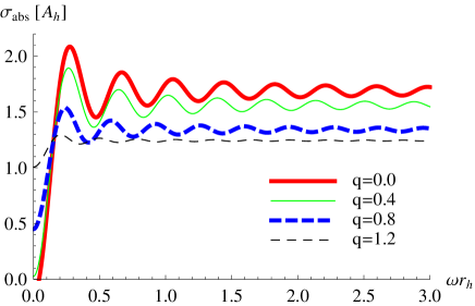
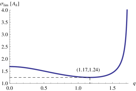
Figure 1: (a) Behavior of the absorption cross section $\sigma_{\text{abs}}$ in units of $A_{\text{h}}=4\pi(1+q^{2})r_{\text{s}}^{2}$. (b) The limiting value $\sigma_{\text{lim}}$ of the absorption cross section in units of $A_{\text{h}}$ vs charge $q$.

From (19), we could see that the absorption cross section has an impact on the energy emission rate. Besides it, the Hawking temperature $T_{\text{H}}$ also has an effect on the energy emission rate. For the JNW solution, the Hawking temperature $T_{\text{H}}$ is calculated as

$$T_{\text{H}}=\frac{1}{4\pi(1+q^{2})r_{\text{s}}}.$$ (25)

When $q=0$, it describes the temperature of the Schwarzschild black hole, i.e., $T^{\text{Sch}}_{\text{H}}=\frac{1}{8\pi M}$. The energy emission rate for it is

$$\frac{d^{2}E(\omega)}{d\omega dt}=\frac{2\pi^{2}\sigma_{\text{abs}}(\omega)}{e^{\frac{\omega}{T_{\text{H}}}}-1}\omega^{3}.$$ (26)

The behavior of the energy emission rate is shown in Fig. 2. The result displays that, when the charge density $q$ increases, the peak of $(r_{\text{h}}\frac{d^{2}E(\omega)}{d\omega dt})$ decreases and the value of $\omega r_{\text{h}}$ corresponding to the peak approaches zero. These results are for the weakly naked singularities. For the marginally and strongly naked singularities, there is no energy emission rate, which means that there is no thermal radiation for these naked singularities, while there is thermal radiation for the weakly naked singularities. With this result and the relation (18), we are allowed to test the cosmic censorship hypothesis through the gravitational lensing by the weakly naked singularities.

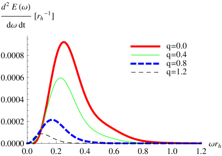
Figure 2: The energy emission rate for the Schwarzschild black hole and the weakly naked singularities.

At the end of this paper, we would like to make a few comments on the possible applications of the relation between the parameters of the strong gravitational lensing and the high-energy absorption cross section in the eikonal regime presented in the current paper. It is clear that, with the observation from the strong gravitational lensing, we can determine the high-energy absorption cross section and energy emission rate for the gravitational source. The data analysis of them may provide us with the range of the frequency for gravitational waves, among which the gravitational source emits the most of its energy. The gravitational waves are most likely to be observed in this range. This result may guide us towards detecting the gravitational waves at a fixed range of the frequency by the gravitational-wave detectors, such as the Laser Interferometer Space Antenna and Laser Interferometer Gravitational-wave Observatory. Furthermore, we also compute the energy emission rate for the Schwarzschild black hole solution and the JNW solution. The results show that, for the weakly naked singularities, there is thermal radiation, which is like that of the Schwarzschild black hole, while, for the marginally and strongly naked singularities, there is no thermal radiation. Thus, these results could provide us with a possible way to test the cosmic censorship hypothesis through the observation of gravitational lensing by the weakly naked singularities acting as gravitational lenses. Another possible application of the result is to determine the dimension $D$ of the spacetime. This may offer us the information about the extra dimensional theories presented in ADD ; RS1 .

The authors are extremely grateful for the anonymous referee, who suggested that the authors compute and compare results for black holes—weakly, marginally, and strongly naked singularities—and whose suggestion helped the authors obtain an important result. This work was supported by the Program for New Century Excellent Talents in University, the Huo Ying-Dong Education Foundation of the Chinese Ministry of Education (No. 121106), and the National Natural Science Foundation of China (No. 11075065).

References

- (1) R. A. Matzner, J. Math. Phys. 9, 163 (1968).
- (2) B. Mashhoon, Phys. Rev. D 7, 2807 (1973).
- (3) A. A. Starobinsky, Sov. Phys. JETP 37, 28 (1973).
- (4) R. Fabbri, Phys. Rev. D 12, 933 (1975).
- (5) D. N. Page, Phys. Rev. D 13, 198 (1976).
- (6) W. G. Unruh, Phys. Rev. D 14, 3251 (1976).
- (7) N. Sanchez, Phys. Rev. D 18, 1030 (1978).
- (8) S. R. Das, G. W. Gibbons, and S. D. Mathur, Phys. Rev. Lett. 78, 417 (1997); J. Maldacena and A. Strominger, Phys. Rev. D 56, 4975 (1997).
- (9) C. W. Misner, K. S. Thorne, and J. A. Wheeler, (W. H. Freeman and Company, San Francisco, 1973).
- (10) Y. Decanini, G. Esposito-Farese, and A. Folacci, Phys. Rev. D 83, 044032 (2011).
- (11) V. Bozza, Gen. Rel. Grav. 42, 2269 (2010).
- (12) K. S. Virbhadra and G. F. R. Ellis, Phys. Rev. D 65, 103004 (2002).
- (13) K. S. Virbhadra and G. F. R. Ellis, Phys. Rev. D 62, 084003 (2000).
- (14) C. Darwin, Proc. R. Soc. London A 249, 180 (1959); 263, 39 (1961); R. D. Atkinson, Astron. J. 70, 517 (1965).
- (15) V. Perlick, Commun. Math. Phys. 220, 403 (2001).
- (16) W. Hasse and V. Perlick, Gen. Relativ. Gravit. 34, 415 (2002); T. Foertsch, W. Hasse, and V. Perlick, Class. Quant. Grav. 20, 4635 (2003).
- (17) K. S. Virbhadra, Phys. Rev. D 79, 083004 (2009).
- (18) S. Chen and J. Jing, Phys. Rev. D 80, 024036 (2009); Y. Liu, S. Chen, and J. Jing, Phys. Rev. D 81, 124017 (2010).
- (19) Y. Decanini and A. Folacci, Phys. Rev. D 81, 024031 (2010).
- (20) I. Z. Stefanov, S. S. Yazadjiev, and G. G. Gyulchev, Phys. Rev. Lett. 104, 251103 (2010).
- (21) C-M. Claudel, K. S. Virbhadra, and G. F. R. Ellis, J. Math. Phys. (N.Y.) 42, 818 (2001).
- (22) V. Perlick, [arXiv:1010.3416[gr-qc]].
- (23) V. Bozza, Phys. Rev. D 66, 103001 (2002).
- (24) V. Bozza and L. Mancini, Gen. Relativ. Gravit. 36, 435 (2004).
- (25) S. W. Hawking, Commun. Math. Phys. 43, 199 (1975).
- (26) A. I. Janis, E. T. Newman, and J. Winicour, Phys. Rev. Lett. 20, 878 (1968).
- (27) K. S. Virbhadra, Int. J. Mod. Phys. A 12, 4831 (1997).
- (28) K. S. Virbhadra, S. Jhingan, and P. S. Joshi, Int. J. Mod. Phys. D 6, 357 (1997).
- (29) K. S. Virbhadra and C. R. Keeton, Phys. Rev. D 77, 124014 (2008).
- (30) K. S. Virbhadra, D. Narasimha, and S. M. Chitre, Astron. Astrophys. 337, 1 (1998).
- (31) N. Arkani-Hamed, S. Dimopoulos, and G. Dvali, Phys. Lett. B 429, 263 (1998).
- (32) L. Randall and R. Sundrum, Phys. Rev. Lett. 83, 3370 (1999); L. Randall and R. Sundrum, Phys. Rev. Lett. 83, 4690 (1999).