Constraint on the early Universe by relic gravitational waves: From pulsar timing observations

Abstract

Recent pulsar timing observations by the Parkers Pulsar Timing Array and European Pulsar Timing Array teams obtained the constraint on the relic gravitational waves at the frequency $f_{*}=1/{\rm yr}$, which provides the opportunity to constrain $H_{*}$, the Hubble parameter when these waves crossed the horizon during inflation. In this paper, we investigate this constraint by considering the general scenario for the early Universe: we assume that the effective (average) equation-of-state $w$ before the big bang nucleosynthesis stage is a free parameter. In the standard hot big-bang scenario with $w=1/3$, we find that the current PPTA result follows a bound $H_{*}\leq 1.15\times 10^{-1}m_{\mathrm{Pl}}$, and the EPTA result follows $H_{*}\leq 6.92\times 10^{-2}m_{\mathrm{Pl}}$. We also find that these bounds become much tighter in the nonstandard scenarios with $w>1/3$. When $w=1$, the bounds become $H_{*}\leq 5.89\times 10^{-3}m_{\mathrm{Pl}}$ for the current PPTA and $H_{*}\leq 3.39\times 10^{-3}m_{\mathrm{Pl}}$ for the current EPTA. In contrast, in the nonstandard scenario with $w=0$, the bound becomes $H_{*}\leq 7.76m_{\mathrm{Pl}}$ for the current PPTA.

I Introduction

A stochastic background of relic gravitational waves, generated during the early inflationary stage, is a necessity dictated by general relativity and quantum mechanics grishchuk1974 ; starobinsky1979 ; mukhanov1992 . The relic gravitational waves have a wide range spreading spectra, and their amplitudes depend only on the Hubble parameter in the inflationary stage, when the waves crossed the horizon, and the expansion history of Universe after the waves reentered the horizon. So their detection provides a direct way to study the physics in the early Universe in both stages, during and after the inflation.

Recently, there have been several experimental efforts to constrain the amplitude of relic gravitational waves in the different frequencies. The current observations of cosmic microwave background (CMB) radiation by the WMAP satellite place an interesting bound on the so-called tensor-to-scalar ratio $r\leq 0.20$ komatsu2011 ; zhaogrishchuk2010 , which is equivalent to the constraint on the energy density $\Omega_{\rm gw}(f)$ of relic gravitational waves at the lowest frequency range $f\sim 10^{-17}$Hz. Among various direct observations, LIGO S5 has also experimentally obtained so far the most stringent bound $\Omega_{\rm gw}(f)\leq 6.9\times 10^{-6}$ around $f\sim 100$Hz ligo2009 . In addition, there are two bounds on the integration $\int\Omega_{\rm gw}(f)d\ln f\mathrel{\hbox{\hbox to0.0pt{\lower 2.36806pt\hbox{$\sim$}\hss} \kern-3.00003pt\raise 1.72218pt\hbox{$<$}}}1.5\times 10^{-5}$, obtained by the Big Bang nucleosynthesis (BBN) observation bbn1999 and the CMB observation cmb2006 . These bounds have been used to constrain the Hubble parameter (or the potential density of inflaton) in the inflationary stage, when the corresponding waves crossed the horizon komatsu2011 ; ligo2009 ; zhang2010 .

The timing studies on the millisecond pulsars provide a unique way to constrain the amplitude of gravitational waves in the frequency range $f\in(10^{-9},10^{-7})$Hz timing . Recently, the Parkers Pulsar Timing Array (PPTA) team and the European Pulsar Timing Array (EPTA) team have reported their observational results on the stochastic background of gravitational waves and given the upper limit of $\Omega_{\rm gw}(f)$ at the frequency $f=1/{\rm yr}$ ppta ; epta . In this paper, we shall infer from these bounds the constraint on $H$, the Hubble parameter at the waves’ horizon-crossing time during inflation. In the calculation, we have considered a general early cosmological model, i.e., we assume the effective (average) equation-of-state $w$ before the BBN stage can be of any value, which includes a wide range of cosmological scenarios. The derived bound of $H$ would limit various inflation models.

II Relic gravitational waves in the standard hot big-bang universe

Incorporating the perturbation to the spatially flat Friedmann-Robertson-Walker (FRW) spacetime, the metric is

$$ds^{2}=a^{2}(\eta)\left[d\eta^{2}-(\delta_{ij}+h_{ij}dx^{i}dx^{j})\right],$$ (1)

where $a$ is the scale factor of the universe, and $\eta$ is the conformal time, which relates to the cosmic time by $ad\eta=dt$. The perturbation of spacetime $h_{ij}$ is a $3\times 3$ symmetric matrix. The gravitational-wave field is the tensorial portion of $h_{ij}$, which is transverse-traceless $\partial_{i}h^{ij}=0$, $\delta^{ij}h_{ij}=0$.

Relic gravitational waves satisfy the linearized evolution equation grishchuk1974 :

$$\partial_{\mu}(\sqrt{-g}\partial^{\mu}h_{ij})=-16\pi G\pi_{ij}.$$ (2)

The anisotropic portion $\pi_{ij}$ is the source term, which can be given by the relativistic free-streaming gas weinberg2003 and the scalar field in the preheating stage preheating . However, it has been deeply discussed that the relativistic free-streaming gas can only affect the relic gravitational waves at the frequency range $f\in(10^{-16},~{}10^{-10})$Hz, which could be detected by the future CMB observations zzx2009 . The generation of stochastic background of gravitational waves in the preheating stage has also been deeply studied (see, for instance, preheating ), where the gravitational radiation was produced in interactions of classical waves created by resonant decay of a coherently oscillating field. However, it was found that the typical frequencies of this kind of gravitational waves are quite high, i.e. $f>10^{4}$Hz. Even if the model with low energy $H\sim 100$GeV is considered, the gravitational waves are important only at the frequency range $f\sim 1$Hz preheating , which could be detected by the future laser interferometer detectors. So, both effects cannot obviously influence the relic gravitational waves at the frequency $f\in(10^{-9},~{}10^{-7})$Hz. For these reasons, in this paper we shall ignore the contribution of the external sources. So the evolution of gravitational waves is only dependent on the scale factor and its time derivative. It is convenient to Fourier transform the equation as follows:

$$h_{ij}(\eta,\vec{x})=\int\frac{d^{3}\vec{k}}{(2\pi)^{3/2}}\sum_{s=+,\times}\left[h_{k}(\eta)\epsilon^{(s)}_{ij}c^{(s)}_{\vec{k}}e^{i\vec{k}\cdot\vec{x}}+c.c.\right],$$ (3)

where $c.c.$ stands for the complex conjugate term. The polarization tensors are symmetry, transverse-traceless $k^{i}\epsilon_{ij}^{(s)}(\vec{k})=0$, $\delta^{ij}\epsilon_{ij}^{(s)}(\vec{k})=0$, and satisfy the conditions $\epsilon^{(s)ij}(\vec{k})\epsilon_{ij}^{(s^{\prime})}(\vec{k})=2\delta_{ss^{\prime}}$ and $\epsilon_{ij}^{(s)}(-\vec{k})=\epsilon_{ij}^{(s)}(\vec{k})$. Since the relic gravitational waves we will consider are isotropy, and each polarization state is the same, we have denoted $h_{\vec{k}}^{(s)}(\eta)$ by $h_{k}(\eta)$, where $k=|\vec{k}|$ is the wavenumber of the gravitational waves, which relates to the frequency by $k\equiv 2\pi f$. (The present scale factor is set $a_{0}=1$). So Eq. (2) can be rewritten as

$${h_{k}}^{\prime\prime}+2\frac{{a^{\prime}}}{a}{h_{k}}^{\prime}+k^{2}h_{k}=0,$$ (4)

where the prime indicates a conformal time derivative $d/d\eta$. For a given wavenumber $k$ and a given time $\eta$, we can define the transfer function $t_{f}$ as

$$t_{f}(\eta,k)\equiv h_{k}(\eta)/h_{k}(\eta_{i}),$$ (5)

where $\eta_{i}$ is the initial conformal time. This transfer function can be obtained by solving the evolution equation (4).

The strength of the gravitational waves is characterized by the gravitational-wave energy spectrum,

$$\Omega_{\rm gw}\equiv\rho_{\rm gw}/\rho_{0},$$ (6)

where $\rho_{\rm gw}=\frac{1}{32\pi G}\langle\dot{h}_{ij}\dot{h}^{ij}\rangle$, the critical density is $\rho_{0}=\frac{3H_{0}^{2}}{8\pi G}$, and $H_{0}=100h\cdot{\rm km}\cdot s^{-1}\cdot{\rm Mpc}^{-1}$ is the current Hubble constant. Using Eqs. (3) and (5), the energy density of gravitational waves can be written as page2006

$$\rho_{\rm gw}=\int\frac{dk}{k}\frac{P_{t}(k)\dot{t}^{2}_{f}(\eta_{0},k)}{32\pi G},$$ (7)

where $P_{t}(k)\equiv\frac{2k^{3}}{\pi^{2}}|h_{k}(\eta_{i})|^{2}$ is the so-called primordial power spectrum of relic gravitational waves. Thus, we derive that the current energy density of relic gravitational waves

$$\Omega_{\rm gw}\equiv\int d\ln{k}~{}\Omega_{\rm gw}(k),{~{}\rm and~{}}\Omega_{\rm gw}(k)=\frac{P_{t}(k)}{12H_{0}^{2}}\dot{t}_{f}^{2}(\eta_{0},k)$$ (8)

where the dot indicates a cosmic time derivative $d/dt$.

Now, let us discuss the terms $P_{t}(k)$ and $t_{f}(\eta_{0},k)$ separately. The primordial power spectrum of relic gravitational waves is usually assumed to be power-law as follows:

$$P_{t}(k)=A_{t}(k_{*})\left(\frac{k}{k_{*}}\right)^{n_{t}}.$$ (9)

This is a generic prediction of a wide range of scenarios of the early Universe, including the inflation models. Here, we should mention that there might be deviations from power-law if we consider the relic gravitational waves in a fairly large wave number span. In this paper, as a conservative consideration, we assume this form is held only when $k$ is very close to the pivot wavenumber $k_{*}$. In the above expression, $n_{t}$ is the spectral index when $k\rightarrow k_{*}$. ($n_{t}=0$ corresponds to the scale-invariant power spectrum.) $A_{t}(k_{*})$ is directly related the value of the Hubble parameter $H$ at time when wavelengths corresponding to the wavenumber $k_{*}$ crossed the horizon grishchuk1974 ; mukhanov1992 ; peiris2003 ,

$$A^{1/2}_{t}(k_{*})=\left.\frac{4}{\sqrt{\pi}}\frac{H_{*}}{m_{\mathrm{Pl}}}\right|_{k_{*}=a_{*}H_{*}},$$ (10)

where $m_{\mathrm{Pl}}\equiv 1/\sqrt{G}$ is the Planck mass.

Now, let us turn to the transfer function $t_{f}$, defined in (5), which describes the evolution of gravitational waves in the expanding Universe. From Eq. (4), we find that this transfer function can be directly derived, so long as the scale factor as a function of time is given. Actually, the analytical or numerical forms of $t_{f}$ have been discussed by a number of authors (see, for instance, grishchuk2000 ; zhang2005 ; tong2009 ; watanabe2006 ).

In this paper, we shall use the following analytical approximation for this transfer function. It has been known that, during the expansion of the Universe, the mode function $h_{k}(\eta)$ of the gravitational waves behaves differently in two regions grishchuk2000 . When waves are far outside the horizon, i.e. $k\ll aH$, the amplitude of $h_{k}$ keeps constant, and when inside the horizon, i.e. $k\gg aH$, the amplitude is damping with the expansion of Universe, i.e., $h_{k}\propto 1/a(\eta)$. In the standard hot big-bang cosmological model, we assume that the inflationary stage is followed by a radiation dominant stage, and then the matter dominant stage and the $\Lambda$ dominant stage. In this scenario, by numerically integrating Eq. (4), one finds that the damping function $\dot{t}_{f}$ can be approximately described by the following form turner1993 ; zhao2006 ; efstathiou2006 ; giovannini2009

$$\dot{t}_{f}(\eta_{0},k)=\frac{-3j_{2}(k\eta_{0})}{k\eta_{0}}\frac{\Omega_{m}}{\Omega_{\Lambda}}\sqrt{1+1.36(\frac{k}{k_{eq}})+2.50(\frac{k}{k_{eq}})^{2}},$$ (11)

where $k_{eq}=0.073\Omega_{m}h^{2}{\rm Mpc}^{-1}$ is the wavenumber corresponding the Hubble radius at the time that matter and radiation have equal energy density, and $\eta_{0}=1.41\times 10^{4}{\rm Mpc}$ is the present conformal time. The factor $\Omega_{m}/\Omega_{\Lambda}$ encodes the damping effect due to the recent accelerating expansion of the Universe zhang2005 ; zhao2006 . In this damping factor, we have ignored the small effects of neutrino free-streaming weinberg2003 and various phase transition watanabe2006 .

We can define a new function

$$\mathcal{T}(k)\equiv\dot{t}_{f}(\eta_{0},k)/\sqrt{12H_{0}^{2}}.$$ (12)

So, the current density of relic gravitational waves becomes $\Omega_{\rm gw}(k)=P_{t}(k)\mathcal{T}^{2}(k)$. In this paper, we shall focus on the wavenumber $k\gg k_{eq}$. In this range, we have zhao2006 ; efstathiou2006 ; giovannini2009

$$\mathcal{T}^{2}(k)=\frac{15}{16}\left(\frac{\Omega_{m}}{\Omega_{\Lambda}}\right)^{2}\frac{1}{H_{0}^{2}\eta_{0}^{4}k_{eq}^{2}}.$$ (13)

and a parameterized form for the current density of relic gravitational waves

$$\Omega_{\rm gw}(k)=\left(\frac{H_{*}}{m_{\mathrm{Pl}}}\right)^{2}\left(\frac{k}{k_{*}}\right)^{n_{t}}\left(\frac{15}{\pi}\frac{1}{H_{0}^{2}\eta_{0}^{4}k_{eq}^{2}}\frac{\Omega_{m}^{2}}{\Omega_{\Lambda}^{2}}\right).$$ (14)

For the wavenumber $k=k_{*}$, the value of $\Omega_{\rm gw}(k_{*})$ depends only on the value of $H_{*}$. So, in this standard scenario, an observational bound on the $\Omega_{\rm gw}(k_{*})$ corresponds to a bound on the Hubble parameter $H_{*}$, which will be shown clearly in Sec. IV.

III Damping factor in the general model of the early universe

Although, in the standard hot big-bang universe, a radiation dominant stage is always assumed after the inflationary stage, there is no observational evidence to show this is held before the BBN stage. Actually, this assumption can be violated in a number of cases, for example, the existence of the reheating stage grishchuk2000 , or the existence of the cosmic phase transition watanabe2006 . So, in general, before the BBN stage, one can assume that the average equation-of-state of the Universe is $w$, and the scale factor satisfies a simple power-law form

$$a\propto\eta^{1+\beta}.$$ (15)

The constant $\beta$ relates to $w$ by $\beta=(-3w+1)/(3w+1)$. Obviously, when $w=1/3$, i.e. $\beta=0$, it returns to the standard model. However, if the Universe is dominated by the kinetic energy of inflaton, one has $w=1$ and $\beta=-1/2$. On the other hand, for a matter dominated era, one has $w=0$ and $\beta=1$.

Now, let us discuss the evolution of relic gravitational waves in this general cosmological model. In principle, it can be done by directly solving Eq. (4). In this paper, in order to avoid the complicated numerical calculation, we give an approximate method as below.

We consider the wave $h_{k}$ with the wavenumber $k$, which crossed the horizon at $a=a_{k}$ and the corresponding Hubble parameter is $H_{k}$. So one has $k=a_{k}H_{k}/a_{0}$. One knows that, when the waves are in the horizon, $h_{k}\propto 1/a(\eta)$, damping with the expansion of the Universe, and when the waves are out the horizon, $h_{k}=constant$, keeping its initial value. So one can define a ratio, which accounts for the damping of the gravitational waves,

$$\frac{h_{k}(\eta_{0})}{h_{k}(\eta_{i})}=\frac{a_{k}}{a_{0}}=\frac{a_{k}}{a_{b}}\frac{a_{b}}{a_{0}},$$ (16)

where $a_{b}$ is the scale factor at the temperature of Universe being $1{\rm MeV}$, i.e. the BBN stage.

In the standard model, where $\beta=0$ in (15) is assumed (i.e. $w=1/3$, the radiation dominant stage), we have

$$\frac{H_{k}}{H_{b}}=\left(\frac{a_{b}}{a_{k}}\right)^{2},$$ (17)

where $H_{b}$ is the Hubble parameter in the BBN stage. Taking into account the relation $k=a_{k}H_{k}/a_{0}$, we obtain that

$$\frac{h_{k}(\eta_{0})}{h_{k}(\eta_{i})}=\frac{a_{b}}{a_{0}}\left(\frac{a_{b}H_{b}}{a_{0}k}\right).$$ (18)

However, in the general case with $\beta\neq 0$, we assume $h_{k}$ crossed the horizon at $a=\tilde{a}_{k}$ and the corresponding Hubble parameter is $\tilde{H}_{k}$. (Note that, in general $\tilde{a}_{k}\neq a_{k}$ and $\tilde{H}_{k}\neq H_{k}$, but $k=\tilde{a}_{k}\tilde{H}_{k}/a_{0}$ is still satisfied.) From the equation in (15), it follows that

$$\frac{\tilde{H}_{k}}{H_{b}}=\left(\frac{a_{b}}{\tilde{a}_{k}}\right)^{\frac{2+\beta}{1+\beta}}.$$

So, in this general case, we have

$$\frac{h_{k}(\eta_{0})}{h_{k}(\eta_{i})}=\frac{\tilde{a}_{k}}{a_{0}}=\frac{a_{b}}{a_{0}}\left(\frac{a_{b}H_{b}}{a_{0}k}\right)^{1+\beta}.$$ (19)

Comparing Eqs. (19) and (18), we can define the damping faction $D(k)$ as follows

$$D(k) \equiv \left(\frac{h_{k}(\eta_{0})}{h_{k}(\eta_{i})}\right)_{general}/\left(\frac{h_{k}(\eta_{0})}{h_{k}(\eta_{i})}\right)_{standard}$$ (20)

$$= \left(\frac{a_{b}H_{b}}{a_{0}H_{0}}\right)^{\beta}\left(\frac{H_{0}}{k_{*}}\right)^{\beta}\left(\frac{k}{k_{*}}\right)^{-\beta}$$ (21)

Thus, in this general scenario, the current density of relic gravitational waves becomes

$$\Omega_{\rm gw}(k)=P_{t}(k)\mathcal{T}^{2}(k)D^{2}(k),$$ (22)

which satisfies $\Omega_{\rm gw}(k)\propto k^{n_{t}-2\beta}$ when $k$ is close to $k_{*}$. Using the formulae in (9), (10), (13), (21), and substituting the cosmological parameters ($h=0.702$, $T_{\rm CMB}=0.276$K, $\Omega_{\Lambda}=0.725$, $\Omega_{m}=0.275$, and $z_{eq}=3454$ )komatsu2011 , we get the following simple result

$$\log_{10}\Omega_{\rm gw}(k_{*})=1.25-\frac{13.48}{3w+1}+2\log_{10}(\frac{H_{*}}{m_{\mathrm{Pl}}}),$$ (23)

where $k_{*}\equiv 2\pi f_{*}$, and $f_{*}=1/{\rm yr}$ is used. In Sec. IV, we shall compare this with the observational results.

IV Constraint by the pulsar timing observations

Pulsar timing observations provide a unique opportunity to study the gravitational waves at the frequency range $f\in(10^{-9},~{}10^{-7}){\rm Hz}$. In 2006, Jenet et al. have analyzed the PPTA data and archival Arecibo data for several millisecond pulsars. By focusing on the gravitational waves with the wavenumer $k_{*}$ (where $k_{*}=2\pi f_{*}$ and $f_{*}=1/{\rm yr}$), and assuming the density of gravitational waves satisfies $\Omega_{\rm gw}(k)=k^{2+2\alpha}$ at around $k\sim k_{*}$, the authors obtained the 2$\sigma$ upper limit on $\Omega_{\rm gw}(k_{*})$ as a function of $\alpha$ ppta , which has been shown in Fig. 1 (black solid line). This figure shows that $\Omega_{\rm gw}(k_{*})\leq 4.05\times 10^{-8}$ when $\alpha=-1$. However, this upper bound increases to be $1.98\times 10^{-6}$ when $\alpha=0$.

Recently, this upper limit has been updated. In epta , the authors have used the current data from the EPTA to determine an upper limit on the stochastic gravitational-wave background as a function of the spectral slope $\alpha$. The 1$\sigma$ and 2$\sigma$ bounds are shown in Fig. 1 (blue lines), which are slightly lower than those in PPTA case for any given $\alpha$.

It is interesting that in ppta , the authors have also investigated the possible upper limit (or a definitive detection) of stochastic background of gravitational waves by using the potential completed PPTA data-sets (20 pulsars with an rms timing residual of 100 ns over 5 years). We have also plotted this potential upper limit in Fig. 1 (red dotted line).

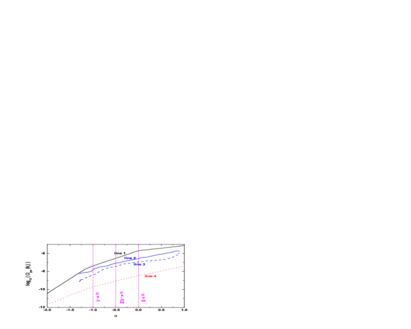
Figure 1: The upper limit of $\Omega_{\rm gw}(k_{*})$ as a function of the parameter $\alpha$. The black solid line (i.e. line 1) is for current PPTA 2$\sigma$ result ppta , the blue solid line (i.e. line 2) is for current EPTA 2$\sigma$ result epta , the blue dashed line (i.e. line 3) is for current EPTA 1$\sigma$ result epta , and the red dotted line (i.e. line 4) is for future PPTA 2$\sigma$ result ppta .

Now, let us compare these observations with the analytical formulae of relic gravitational waves in Sec. III. Firstly, it is necessary to relate the parameter $\alpha$ with the theoretical models. In Sec. III, Eq. (22) shows that $\Omega_{\rm gw}(k)\propto k^{n_{t}-2\beta}$, where $\beta=(-3w+1)/(3w+1)$. Comparing this with the assumed form $\Omega_{\rm gw}(k)\propto k^{2+2\alpha}$, we get the interesting relation

$$\alpha=\frac{n_{t}}{2}-\frac{2}{3w+1}.$$ (24)

This relation shows that, in the standard hot big-bang scenario with $w=1/3$, and the scale-invariant primordial power spectrum with $n_{t}=0$, we have $\alpha=-1$. In this case, let us use the bounds of gravitational waves to constrain the Hubble parameter $H_{*}$ in the inflationary stage. Taking into account the formula in Eq. (23) and using $w=1/3$, we obtain the 2$\sigma$ upper limit of $H_{*}$, i.e. $H_{*}\leq 1.15\times 10^{-1}m_{\mathrm{Pl}}$ for the current PPTA case, $H_{*}\leq 6.92\times 10^{-2}m_{\mathrm{Pl}}$ for the current EPTA case, and the future PPTA is expected to give $H_{*}\leq 7.94\times 10^{-3}m_{\mathrm{Pl}}$. These results are listed in Table 1.

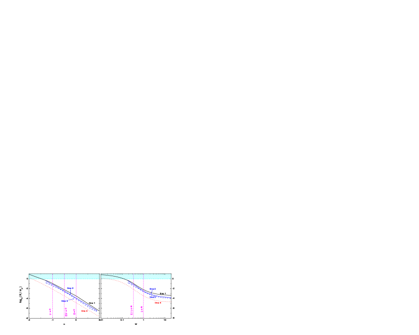
Figure 2: The upper limit of the Hubble parameter $H_{*}$ as a function of the parameter $\alpha$ (left panel) and the average equation-of-state $w$ (right panel), where we have assumed $n_{t}=0$. In both panels, the black solid lines (i.e. line 1) are for current PPTA 2$\sigma$ result, the blue solid lines (i.e. line 2) are for current EPTA 2$\sigma$ result, the blue dashed lines (i.e. line 3) are for current EPTA 1$\sigma$ result, and the red dotted lines (i.e. line 4) are for future PPTA 2$\sigma$ result.

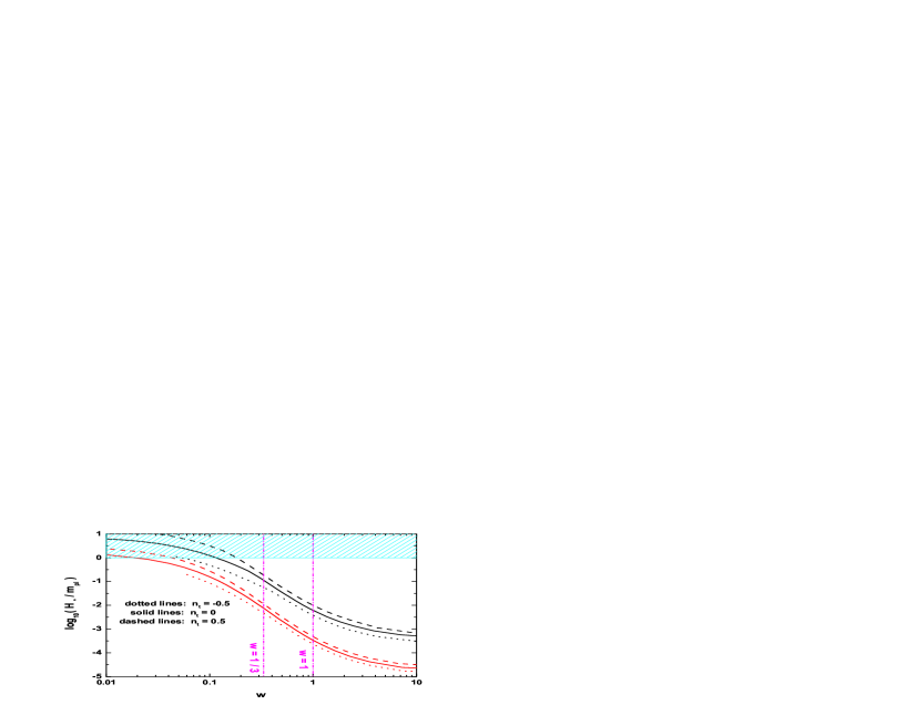
Figure 3: The upper limit of the Hubble parameter $H_{*}$ as a function of the average equation-of-state $w$, where we have considered three cases with $n_{t}=-0.5$, $0$, $0.5$. The black lines are for current PPTA 2$\sigma$ result, and the red lines are for future PPTA 2$\sigma$ result.

Although, the inflation models always predict the nearly same Hubble parameter throughout the inflationary stage, it is necessary to constrain $H$, the Hubble parameter at quite different stages of inflation, which encodes the evolution information of inflaton. Here, let us compare the bound of $H$ inferred from pulsar timing with those obtained in CMB observations and LIGO observations. The recent CMB observations by the WMAP satellite provide the constraint on the tensor-to-scalar ratio $r\leq 0.20$ komatsu2011 , which is equivalent to the bound of $H/m_{\mathrm{Pl}}\leq 6.92\times 10^{-6}$, where $H$ is the Hubble parameter of inflation when the waves with frequency $f=1.94\times 10^{-17}$Hz crossed the horizon. The recent LIGO 5S reported so far the tightest constraint $\Omega_{\rm gw}(f)\leq 6.9\times 10^{-6}$ on relic gravitational waves at the frequency $f\simeq 100$Hz ligo2009 , which corresponds to $H/m_{\mathrm{Pl}}\leq 1.46$. Comparing with these results, we find that the current and the potential future pulsar timing constraints on $H$ are quite tighter than that of LIGO, but much looser than the CMB constraint.

Table 1: The 2$\sigma$ upper limit of the quantity $H_{*}/m_{\mathrm{Pl}}$ inferred from various pulsar timing observations. In this table, we have assumed $n_{t}=0$.

	Current PPTA	Current EPTA	Future PPTA
$w=0$	$7.76$	……	$1.41$
$w=1/3$	$1.15\times 10^{-1}$	$6.92\times 10^{-2}$	$7.94\times 10^{-3}$
$w=1$	$5.89\times 10^{-3}$	$3.39\times 10^{-3}$	$3.55\times 10^{-4}$
$w\rightarrow\infty$	$3.16\times 10^{-4}$	$1.20\times 10^{-4}$	$1.41\times 10^{-5}$

Now, let us relax the assumptions of the early Universe. We only assume $n_{t}=0$, which is approximately held in a wide range of inflation models. So, we can constrain the Hubble parameter $H_{*}$ in a wide range of $w$ by the following inequality

$$\log_{10}(\frac{H_{*}}{m_{\mathrm{Pl}}})\leq\frac{1}{2}(U(\alpha)-6.74\alpha-1.25),$$ (25)

where $U(\alpha)$ is the upper limit of $\Omega_{\rm gw}(k_{*})$ based on the pulsar timing observations, which is a function of the parameter $\alpha$ (in this case, $\alpha$ relates to $w$ by the relation $\alpha=-2/(3w+1)$). The bounds of $H_{*}$ as functions of $\alpha$ (left panel) and $w$ (right panel) are shown in Fig. 2. These bounds in three special cases with $w=0$ (i.e. $\alpha=-2$), $w=1$ (i.e. $\alpha=-1/2$) and $w\rightarrow\infty$ (i.e. $\alpha=0$) are also listed in Table 1. Clearly, we find that a larger $w$ corresponds to a tighter bound of $H_{*}$. Especially, in the limit case with $w\rightarrow\infty$, the current EPTA gives the constraint $H_{*}\leq 1.20\times 10^{-4}m_{\mathrm{Pl}}$, and the future PPTA is expected to give a bound of $H_{*}\leq 1.41\times 10^{-5}m_{\mathrm{Pl}}$.

In the end, let us discuss the most general case with free parameters $n_{t}$ and $w$. In this case, the inequality (25) becomes the constraint on the physical parameters $n_{t}$ and $H_{*}$ as follows

$$\log_{10}(\frac{H_{*}}{m_{\mathrm{Pl}}})-1.69n_{t}\leq\frac{1}{2}(U(\alpha)-6.74\alpha-1.25).$$ (26)

Here, we should remember that $\alpha$ relates to the physical parameters by Eq. (24). The spectra index $n_{t}$ influences the bound of $H_{*}$ mainly by slight changing the corresponding relation between $\alpha$ and $w$. In Fig. 3, we calculate the upper bound of $H_{*}$ in two special cases with $n_{t}=0.5$ and $n_{t}=-0.5$, and compare them with those in the case of $n_{t}=0$. This figure shows that the parameter $n_{t}$ only slightly affects the bound of $H_{*}$, and a larger $n_{t}$ follows a looser bound of $H_{*}$. For example, the current PPTA observations follow $H_{*}\leq 1.82\times 10^{-1}m_{\mathrm{Pl}}$ at the case with $n_{t}=0.5$ and $w=0$, which is only $1.6$ times larger than the bound $H_{*}\leq 1.14\times 10^{-1}m_{\mathrm{Pl}}$ at the case with $n_{t}=0$ and $w=0$.

Acknowledgements: This work is supported by NSFC Grant Nos.10703005, 10775119 and 11075141.

References

- (1) L. P. Grishchuk, Sov. Phys. JETP 40, 409 (1975); Ann. N. Y. Acad. Sci. 302, 439 (1977); JETP Lett. 23, 293 (1976);
- (2) A. A. Starobinsky, JETP Lett. 30, 682 (1979); Phys. Lett. B91, 99 (1980).
- (3) A. D. Linde, Phys. Lett. B108, 389 (1982); A. Albrecht and P. J. Steinhardt, Phys. Rev. Lett. 48, 1220 (1982); V. F. Mukhanov, H. A. Feldman, and R. H. Brandenberger, Phys. Rep. 215, 203 (1992); D. H. Lyth and A. Riotto, Phys. Rep. 314, 1 (1999).
- (4) E. Komatsu et al., Astrophys. J. Suppl. Ser. 192, 18 (2011).
- (5) W. Zhao and L. P. Grishchuk, Phys. Rev. D82, 123008 (2010); W. Zhao, Phys. Rev. D79, 063003 (2009).
- (6) B. P. Abbott et al., [LIGO Scientific Collaboration and Virgo Collaboration], Nature, 460, 990 (2009).
- (7) B. Allen and J. D. Romano, Phys. Rev. D59, 102001 (1999).
- (8) T. L. Smith, E. Pierpaoli, and M. Kamionkowski, Phys. Rev. Lett. 97, 021301 (2006).
- (9) Y. Zhang, M. L. Tong and Z. W. Fu, Phys. Rev. D81, 101501(R) (2010).
- (10) S. Detweiler et al., Astrophys. J. 234, 1100 (1979); R. Hellings and G. Downs, Astrophys. J. 265, L39 (1983).
- (11) F. Jenet et al., Astrophys. J. 653, 1571 (2006).
- (12) R. van Haasteren et al., arXiv:1103.0576.
- (13) S. Weinberg, Phys. Rev. D69, 023503 (2004).
- (14) S. Y. Khlebnikov and I. I. Tkachev, Phys. Rev. D56, 653 (1997); J.Garcia-Bellido and D. G. Figueroa, Phys. Rev. Lett. 98, 061302 (2007).
- (15) W. Zhao, Y. Zhang and T. Y. Xia, Phys. Lett. B677, 235 (2009).
- (16) L. Pages et al., Astrophys. J. Suppl. Ser. 170, 335 (2007).
- (17) H. V. Peiris et al., Astrophys. J. Suppl. Ser. 148, 213 (2003).
- (18) L. P. Grishchuk, Lect. Notes Phys. 562, 167 (2001).
- (19) Y. Zhang, Y. F. Yuan, W. Zhao and Y. T. Chen, Class. Quant. Grav. 22, 1383 (2005).
- (20) M. L. Tong and Y. Zhang, Phys. Rev. D80, 084022 (2009).
- (21) Y. Watanabe and E. Komatsu, Phys. Rev. D73, 123515 (2006).
- (22) W. Zhao and Y. Zhang, Phys. Rev. D74, 043503 (2006).
- (23) M. S. Turner, M. White and J. E. Lidsey, Phys. Rev. D48, 4613 (1993).
- (24) S. Chongchitnan and G. Efstathiou, Phys. Rev. D73 083511 (2006).
- (25) M. Giovannini, PMC Phys. A4, 1 (2010).