Complementarity of Semileptonic $B$ to $K_{2}^{*}(1430)$ and $K^{*}(892)$ Decays in the Standard Model with Fourth Generation

Abstract

The $B\rightarrow K_{2}^{\ast}(1430)l^{+}l^{-}$ $(l=\mu,\tau)$ decays are analyzed in the Standard Model extended to fourth generation of quarks (SM4). The decay rate, forward-backward asymmetry, lepton polarization asymmetries and the helicity fractions of the final state $K^{*}_{2}(1430)$ meson are obtained using the form factors calculated in the light cone sum rules (LCSR) approach. We have utilized the constraints on different fourth generation parameters obtained from the experimental information on $K$, $B$ and $D$ decays and from the electroweak precision data to explore their impact on the $B\rightarrow K_{2}^{\ast}(1430)l^{+}l^{-}$ decay. We find that the values of above mentioned physical observables deviate deviate significantly from their minimal SM predications. We also identify a number of correlations between various observables in $B\rightarrow K_{2}^{\ast}(1430)l^{+}l^{-}$ and $B\rightarrow K^{\ast}(892)l^{+}l^{-}$ decays. Therefore a combined analysis of these two decays will compliment each other in the searches of SM4 effects in flavor physics.

I Introduction

The standard model has been tested to a high degree of precision and the only missing link is the Higgs scalar. Apart from the direct search for Higgs at LHC, the other purpose of LHC is to test the various extensions of the standard model such as supersymmetry, extra dimensions, technicolor, neutral vector boson $Z^{\prime}$ and standard model with fourth generation of quarks and leptons (SM4). The search for new degrees of freedom at LHC can be done in two distinct ways. One is the direct search of the Higgs boson and the particles beyond the SM to establish the new physics (NP) theories. The other is the indirect way where we test the SM with high theoretical and experimental precision for which the rare $B$ meson decays are an ideal probe. Among different $B$ meson decays the one which proceed through Flavor Changing Neutral Current (FCNC) transitions, like $b\rightarrow s\gamma$ and $b\rightarrow sl^{+}l^{-}$, are of special interest. This lies in the fact that FCNC transitions generally arise at loop level in the SM, and thus provide a good testing ground for the various extensions of the SM.

The radiative decays $b\rightarrow s\gamma$ and $B\rightarrow K^{\ast}(892)\gamma$ are easy to calculate but they have limited physical observables in comparison to the semileptonic $B\rightarrow K^{\ast}(892)l^{+}l^{-}(l=\mu,\tau)$ decay. In semileptonic decays one can study number of physical observables like decay rate, forward-backward asymmetries, lepton polarization asymmetries and the isospin symmetries. The theoretical research in these semileptonic decay modes has been done with highly improved precision, see Ref. semileptonic , with good support from their experimental studies at B factories and the hadron colliders experiment1 . With the start of LHC we are expecting better statistics, the LHCb experiment can accumulate 6200 events per nominal running year at $14$ TeV experiment2 . The sensitivity of measuring the zero-position of the forward-backward asymmetry at LHC will reduce to $0.5GeV^{2}$ which may be further improved to $0.1GeV^{2}$ after the upgrade experiment3 . Hence, its investigation will not only provide us an opportunity to discriminate between the SM and different NP models but will also improve our understanding of the short-distance physics at an unprecedented level.

The experimental observation of the $B\rightarrow K_{2}^{\ast}(1430)\gamma$ decay at BaBar and Belle babar-belle indicates that its branching ratio is comparable to $B\rightarrow K^{\ast}(892)\gamma$. The related decay mode with photon in the final state replaced by a pair of charged leptons has already been seen for $K^{\ast}(892)$. Like $B\rightarrow K^{\ast}(892)l^{+}l^{-}$ the decay $B\rightarrow K_{2}^{\ast}(1430)l^{+}l^{-}$ is also described by the quark level transition $b\to sl^{+}l^{-}$ and hence the same NP would be expected to affect their measurements. Therefore, the analysis of $B\rightarrow K_{2}^{\ast}(1430)l^{+}l^{-}$ process will usefully complement the much investigated decay process $B\rightarrow K^{\ast}(892)l^{+}l^{-}$ semileptonic . The experimental observation of this decay will provide some supplementary tests of the predictions of SM btotensor .

It has already been mentioned that the unitarity of quark mixing matrix forbids the FCNC transitions at tree level in the SM. When loop corrections are taken into account, $b\to sl^{+}l^{-}$ arises from the photon penguin, $Z$ penguin and the $W$-box diagrams. The large mass scale of virtual states leads to tiny Wilson coefficients in $b$ quark decays and thus $b\to sl^{+}l^{-}$ would be sensitive to the potential NP effects Wei . These NP effects enter in two distinct ways: in one scenario new operators not present in SM can emerge while in other scenario only the Wilson coefficients of the SM operators get modified. SM with an extra generation of quarks is one of the simplest scenario of the later category and recently it has attracted an increasing interest (see ref. hurth for brief review on SM4). In this work we study its impact on $B\rightarrow K_{2}^{\ast}(1430)l^{+}l^{-}(l=\mu,\tau)$ decays.

The electroweak precision data does not exclude the complete existence of the fourth family and there are many reasons to introduce an extra generation of heavy particles soni-hou . Especially, LHC has a potential to discover or fully exclude the existence of a fourth generation of quarks up to 1 TeV hurth . Even if they are too heavy to be observed directly they will induce a large signal in $gg\to ZZ$ which will be clearly visible at the LHC chanowitz .

The sequential fourth generation model is a simple and non-supersymmetric extension of the SM, which does not add any new dynamics to the SM, with an additional up-type quark $t^{\prime}$ and down-type quark $b^{\prime}$ , a heavy charged lepton $\tau^{\prime}$ and an associated neutrino $\nu^{\prime}$. Being a simple extension of the SM it retains all the properties of the SM where the new top quark $t^{\prime}$ like the other up-type quarks, contributes to $b\to s$ transition at the loop level. Due to the additional fourth generation the quark mixing matrix (CKM) will become $4\times 4$, i.e.,

$$V_{\text{CKM4}}=\left(\begin{array}[]{cccc}V_{ud}&V_{us}&V_{ub}&V_{ub^{\prime}}\\ V_{cd}&V_{cs}&V_{cb}&V_{cb^{\prime}}\\ V_{td}&V_{ts}&V_{tb}&V_{tb^{\prime}}\\ V_{t^{\prime}d}&V_{t^{\prime}s}&V_{t^{\prime}b}&V_{t^{\prime}b^{\prime}}\end{array}\right)$$ (1)

where $V_{qb^{\prime}}$ and $V_{t^{\prime}q}$ are new matrix elements in the SM4. The parametrization of this unitary matrix requires six mixing angles and three phases [9]. The effects of sequential fourth generation have already been studied on different physical observables in $B$, $K$ and $D$ decays, see ref. reviews for a short list.

In this work, we analyze the possible fourth generation effects on the decay rates, forward-backward asymmetry $(A_{FB})$, the final state lepton polarization asymmetries $(P_{L,N,T})$ and the helicity fractions of $K^{\ast}_{2}(1430)$ meson $(f_{L,T})$ in $B\rightarrow K_{2}^{\ast}(1430)l^{+}l^{-}(l=\mu,\tau)$ decays. It is well known that the constraints on the NP parameters in $b\to sl^{+}l^{-}$ are obtained mainly from the related decay modes $B\to X_{s}l^{+}l^{-}$ and the golden channel $B_{s}\to\mu^{+}\mu^{-}$. Due to the large hadronic uncertainties, the exclusive decays (under discussion here) $B\to(K^{\ast}(892),K_{2}^{\ast}(1430))l^{+}l^{-}$ provide weaker constraints than the inclusive decay modes $B\to X_{s}l^{+}l^{-}$. Clearly our aim here is not to obtain the precise predictions of the SM4 but rather to obtain an understanding of how NP arising from the SM4 affects different physical observables.

In these FCNC transitions the fourth generation top quark $t^{\prime}$, like $u$, $c$, $t$ quarks, contributes at loop level which result in the modification of the corresponding Wilson coefficients. In our numerical study of $B\rightarrow K_{2}^{\ast}(1430)l^{+}l^{-}$ decays, we shall use the the form factors calculated using LCSR approach in Ref. LCSR . By incorporating the recent constraints on the fourth generation parameters, $m_{t^{\prime}}=300-600$ GeV and $V_{t^{\prime}b}V_{t^{\prime}s}=\left(0.05-1.4\right)\times 10^{-2}$ Gupta-soni ; CDFNEW ; CDF ; Londonnewsm4 ; boundsCKM ; Samitra ; boundsSM3 ; boundsSM4 , our results show that the decay rates of $B\rightarrow K_{2}^{\ast}(1430)l^{+}l^{-}(l=\mu,\tau)$ are quite sensitive to these parameters. The NP effects in the decay rate are usually masked by the uncertainties associated with the different input parameters especially arising from the form factors. Therefore, one has to look for the observables which have mild dependence on these form factors. The zero position of FBA, lepton polarization asymmetries and helicity fractions of final state mesons are efficient tools to search for NP. We have studied these asymmetries in the SM4 and found that the effects of fourth generation parameters are quite significant in some regions of parameter space of the SM4. A qualitative comparison of the results of different physical observables of decays $B\to K_{2}^{\ast}(1430)l^{+}l^{-}$ and $B\to K^{\ast}(892)l^{+}l^{-}$ will show that these two decays will compliment each other for certain physical observables.

The paper is organized as follows. In Sec. II, we present the effective Hamiltonian for the semileptonic decay $B\rightarrow K_{2}^{\ast}(1430)l^{+}l^{-}$, Section III contains the definitions and the numerical values of the form factors. In Sec. IV we present the expressions of physical observables under discussion here. Section V is devoted to the numerical analysis where we analyze the sensitivity of these physical observables on fourth generation parameter $\left(m_{t^{\prime}}\text{, }V_{t^{\prime}b}^{\ast}V_{t^{\prime}s}\right)$. Finally, the main results are summarized in Sec. VI.

II Effective Hamiltonian and Matrix Elements

In the Standard Model (SM3) the $B\rightarrow K_{2}^{\ast}(1430)$ transition is governed by the effective Hamiltonian

$$H_{eff}=-\frac{4G_{F}}{\sqrt{2}}V_{tb}^{\ast}V_{ts}{\sum\limits_{i=1}^{10}}C_{i}({\mu})O_{i}({\mu}),$$ (2)

where $O_{i}({\mu})$ $(i=1,\ldots,10)$ are the four-quark operators and $C_{i}({\mu})$ are the corresponding Wilson coefficients at the energy scale ${\mu}$. Currently these Wilson coefficients are calculated in the SM at Next-to-Leading Order (NLO) and Next-to-Next Leading Logarithm (NNLL) and their explicit expressions are given in the literature Buchalla ; Buras ; Kim ; Ali ; Kruger ; Grinstein ; Cella ; Bobeth ; Asatrian ; Misiak ; Huber . Out of these 10 operators the ones which are responsible for $B\rightarrow K_{2}^{\ast}(1430)l^{+}l^{-}$ are $O_{7}$, $O_{9}$ and $O_{10}$ and their form is given below

$$O_{7} = \frac{e^{2}}{16\pi^{2}}m_{b}\left(\bar{s}\sigma_{\mu\nu}P_{R}b\right)F^{\mu\nu},\,$$

$$O_{9} = \frac{e^{2}}{16\pi^{2}}(\bar{s}\gamma_{\mu}P_{L}b)(\bar{l}\gamma^{\mu}l),\,$$ (3)

$$O_{10} = \frac{e^{2}}{16\pi^{2}}(\bar{s}\gamma_{\mu}P_{L}b)(\bar{l}\gamma^{\mu}\gamma_{5}l),$$

with $P_{L,R}=\left(1\pm\gamma_{5}\right)/2$. In terms of the above operators, the free quark decay amplitude for $b\rightarrow s$ $l^{+}l^{-}$ in the SM can be derived as:

$$\mathcal{M}(b \rightarrow sl^{+}l^{-})=-\frac{G_{F}\alpha}{\sqrt{2}\pi}V_{tb}V_{ts}^{\ast}\bigg{\{}C_{9}^{eff}(\mu)(\bar{s}\gamma_{\mu}P_{L}b)(\bar{l}\gamma^{\mu}l)+C_{10}(\bar{s}\gamma_{\mu}P_{L}b)(\bar{l}\gamma^{\mu}\gamma_{5}l)$$ (4)

$$-2m_{b}C_{7}^{eff}(\mu)(\bar{s}i\sigma_{\mu\nu}\frac{q^{\nu}}{q^{2}}P_{R}b)(\bar{l}\gamma^{\mu}l)\bigg{\}},$$

where $q^{2}$ is the square of the momentum transfer. The operator $O_{10}$ can not be induced by the insertion of four-quark operators because of the absence of the $Z$ -boson in the effective theory. Therefore, the Wilson coefficient $C_{10}$ does not renormalize under QCD corrections and hence it is independent of the energy scale. In addition to this, the above quark level decay amplitude can receive contributions from the matrix elements of four-quark operators, $\sum_{i=1}^{6}\langle l^{+}l^{-}s|O_{i}|b\rangle$, which are usually absorbed into the effective Wilson coefficient $C_{9}^{SM}(\mu)$, usually called $C_{9}^{eff}$, which can be decomposed into the following three parts

$$C_{9}^{SM}(\mu)\equiv C_{9}^{eff}(\mu)=C_{9}(\mu)+Y_{SD}(z,s^{\prime})+Y_{LD}(z,s^{\prime}),$$

where the parameters $z$ and $s^{\prime}$ are defined as $z=m_{c}/m_{b},\,\,\,s^{\prime}=q^{2}/m_{b}^{2}$. $Y_{SD}(z,s^{\prime})$ describes the short-distance contributions from four-quark operators far away from the $c\bar{c}$ resonance regions, which can be calculated reliably in the perturbative theory. The long-distance contributions $Y_{LD}(z,s^{\prime})$ from four-quark operators near the $c\bar{c}$ resonance cannot be calculated from first principles of QCD and are usually parameterized in the form of a phenomenological Breit-Wigner formula making use of the vacuum saturation approximation and quark-hadron duality. We will neglect the long-distance contributions in this work because of the absence of experimental data on $B\rightarrow J/\psi K_{2}^{\ast}(1430)$ and also the NP effects lie far from the resonance region. The explicit expressions for $Y_{SD}(z,s^{\prime})$ can be written as Buras

$$Y_{SD}(z,s^{\prime}) = h(z,s^{\prime})(3C_{1}(\mu)+C_{2}(\mu)+3C_{3}(\mu)+C_{4}(\mu)+3C_{5}(\mu)+C_{6}(\mu))$$ (5)

$$-\frac{1}{2}h(1,s^{\prime})(4C_{3}(\mu)+4C_{4}(\mu)+3C_{5}(\mu)+C_{6}(\mu))$$

$$-\frac{1}{2}h(0,s^{\prime})(C_{3}(\mu)+3C_{4}(\mu))+{\frac{2}{9}}(3C_{3}(\mu)+C_{4}(\mu)+3C_{5}(\mu)+C_{6}(\mu)),$$

with

$$h(z,s^{\prime}) = -{\frac{8}{9}}\mathrm{ln}z+{\frac{8}{27}}+{\frac{4}{9}}x-{\frac{2}{9}}(2+x)|1-x|^{1/2}\left\{\begin{array}[]{l}\ln\left|\frac{\sqrt{1-x}+1}{\sqrt{1-x}-1}\right|-i\pi\quad\mathrm{for}{{\ }x\equiv 4z^{2}/s^{\prime}<1}\\ 2\arctan\frac{1}{\sqrt{x-1}}\qquad\mathrm{for}{{\ }x\equiv 4z^{2}/s^{\prime}>1}\end{array}\right.,$$ (8)

$$h(0,s^{\prime}) = {\frac{8}{27}}-{\frac{8}{9}}\mathrm{ln}{\frac{m_{b}}{\mu}}-{\frac{4}{9}}\mathrm{ln}s^{\prime}+{\frac{4}{9}}i\pi\,\,.$$ (9)

Apart from the correction to $C_{9}^{SM}$, the non-factorizable effects b to s 1 ; b to s 2 ; b to s 3 ; NF charm loop from the charm loop can bring about further corrections to the radiative $b\rightarrow s\gamma$ transition, which can be absorbed into the effective Wilson coefficient $C_{7}^{eff}$. Specifically, the Wilson coefficient $C_{7}^{eff}$ is given by c.q. geng 4

$$C_{7}^{SM}(\mu)=C_{7}^{eff}(\mu)=C_{7}(\mu)+C_{b\rightarrow s\gamma}(\mu),$$

with

$$C_{b\rightarrow s\gamma}(\mu) = i\alpha_{s}\bigg{[}{\frac{2}{9}}\eta^{14/23}(G_{1}(x_{t})-0.1687)-0.03C_{2}(\mu)\bigg{]},$$ (10)

$$G_{1}(x_{t}) = {\frac{x_{t}(x_{t}^{2}-5x_{t}-2)}{8(x_{t}-1)^{3}}}+{\frac{3x_{t}^{2}\mathrm{ln}^{2}x_{t}}{4(x_{t}-1)^{4}}},$$ (11)

where $\eta=\alpha_{s}(m_{W})/\alpha_{s}(\mu)$, $x_{t}=m_{t}^{2}/m_{W}^{2}$, $C_{b\rightarrow s\gamma}$ is the absorptive part for the $b\rightarrow sc\bar{c}\rightarrow s\gamma$ rescattering and we have dropped out the tiny contributions proportional to CKM sector $V_{ub}V_{us}^{\ast}$. In addition, $C_{7}^{new}(\mu)$ can be obtained by replacing $m_{t}$ with $m_{t\prime}$ in the above expression. Similar replacement $(m_{t}\rightarrow m_{t^{\prime}})$ has to be done for the other Wilson Coefficients $C_{9}^{eff}$ and $C_{10}$ which have too lengthy expressions to be given here and their explicit expressions are given in refs. Buchalla ; Buras ; Kim ; Ali ; Kruger ; Grinstein ; Cella ; Bobeth ; Asatrian ; Misiak ; Huber .

It has already been pointed out that the sequential fourth generation does not change the operator basis of the SM, therefore, its effects will change the values of the Wilson coefficients $C_{7}\left(\mu\right)$, $C_{9}\left(\mu\right)$ and $C_{10}$ via the virtual exchange of new generation up-type quark $t^{\prime}$. The modified Wilson coefficients will take the form;

$$\lambda_{t}C_{i}\rightarrow\lambda_{t}C_{i}^{SM}+\lambda_{t^{\prime}}C_{i}^{new},$$ (12)

where $\lambda_{f}=V_{fb}^{\ast}V_{fs}$ $(f,t,t^{\prime})$ and the explicit forms of the $C_{i}$’s can be obtained from the corresponding expressions of the Wilson coefficients in SM by putting $m_{t}\rightarrow m_{t^{\prime}}$. The addition of an extra family of quarks will also add an extra row and a column in the CKM matrix of the SM which now becomes $4\times 4$ and the unitarity of which leads to

$$\lambda_{u}+\lambda_{c}+\lambda_{t}+\lambda_{t^{\prime}}=0,$$ (13)

Since $\lambda_{u}=V_{ub}^{\ast}V_{us}$ has a very small value compared to the other CKM matrix elements, therefore, it is safe to ignore it. Thus from Eq. (13) we have

$$\lambda_{t}\approx-\lambda_{c}-\lambda_{t^{\prime}}$$ (14)

which by plugging in Eq. (12) gives

$$\lambda_{t}C_{i}^{SM}+\lambda_{t^{\prime}}C_{i}^{new}=-\lambda_{c}C_{i}^{SM}+\lambda_{t^{\prime}}\left(C_{i}^{new}-C_{i}^{SM}\right).$$ (15)

Here, one can clearly see that under $\lambda_{t^{\prime}}\rightarrow 0$ or $m_{t^{\prime}}\rightarrow m_{t}$ the term $\lambda_{t^{\prime}}\left(C_{i}^{new}-C_{i}^{SM}\right)$ vanishes which is the requirement of GIM mechanism. After including the $t^{\prime}$ quark in the loop the relevant Wilson coefficients $C_{7},C_{9}$ and $C_{10}$ can take the following form

$$C_{7}^{tot}\left(\mu\right) = C_{7}^{SM}\left(\mu\right)+\frac{\lambda_{t^{\prime}}}{\lambda_{t}}C_{7}^{new}\left(\mu\right),$$

$$C_{9}^{tot}\left(\mu\right) = C_{9}^{SM}\left(\mu\right)+\frac{\lambda_{t^{\prime}}}{\lambda_{t}}C_{9}^{new}\left(\mu\right),$$ (16)

$$C_{10}^{tot} = C_{10}^{SM}+\frac{\lambda_{t^{\prime}}}{\lambda_{t}}C_{10}^{new},$$

We recall here that the the CKM coefficient corresponding to the $t$-quark contribution, i.e,. $\lambda_{t}$ is factorized in the effective Hamiltonian given in Eq. (2) and the Wilson coefficients $C_{i}^{SM}$ corresponds to the ones which appear in Eq. (2). Now $\lambda_{t^{\prime}}$ can be parameterized as:

$$\lambda_{t^{\prime}}=\left|V_{t^{\prime}b}^{\ast}V_{t^{\prime}s}\right|e^{i\phi_{sb}}$$ (17)

where $\phi_{sb}$ is the phase factor corresponding to the $b\rightarrow s$ transition in SM4 which was taken to be $90^{\circ}$ phase in the forthcoming numerical analysis of different physical observables. In terms of the above SM4 Wilson coefficients, the free quark decay amplitude for $b\rightarrow s$ $l^{+}l^{-}$ becomes:

$$\mathcal{M}(b \rightarrow sl^{+}l^{-})=-\frac{G_{F}\alpha}{\sqrt{2}\pi}V_{tb}V_{ts}^{\ast}\bigg{\{}C_{9}^{tot}(\mu)(\bar{s}\gamma_{\mu}P_{L}b)(\bar{l}\gamma^{\mu}l)+C_{10}^{tot}(\bar{s}\gamma_{\mu}P_{L}b)(\bar{l}\gamma^{\mu}\gamma_{5}l)$$ (18)

$$-2m_{b}C_{7}^{tot}(\mu)(\bar{s}i\sigma_{\mu\nu}\frac{q^{\nu}}{q^{2}}P_{R}b)(\bar{l}\gamma^{\mu}l)\bigg{\}}.$$

III Matrix Elements and Form Factors

With the free quark amplitude available (c.f. Eq. (18)), one can proceed to calculate the amplitudes for the exclusive semi-leptonic $B\rightarrow K_{2}^{\ast}(1430)l^{+}l^{-}$ decay, which can be obtained by sandwiching the free quark amplitudes between the initial and final meson states. In general these matrix elements can be parameterized in term of the form factors as follows:

$$\left\langle K_{2}^{\ast}(k,\epsilon)\left|\overline{s}\gamma^{\mu}b\right|\overline{B}(p)\right\rangle = -\frac{2V(q^{2})}{m_{B}+m_{K_{2}^{\ast}}}\epsilon^{\mu\nu\rho\sigma}\frac{\varepsilon_{\nu\alpha}^{\ast}p^{\alpha}}{m_{B}}p_{\rho}k_{\sigma}$$ (19)

$$\left\langle K_{2}^{\ast}(k,\epsilon)\left|\overline{s}\gamma^{\mu}\gamma^{5}b\right|\overline{B}(p)\right\rangle = \frac{2im_{K_{2}^{\ast}}A_{0}(q^{2})}{q^{2}}\frac{\varepsilon_{\nu\alpha}^{\ast}p^{\alpha}}{m_{B}}q^{\nu}q^{\mu}+\frac{i(m_{B}+m_{K_{2}^{\ast}})A_{1}(q^{2})}{m_{B}}\left[g^{\mu\nu}\varepsilon_{\nu\alpha}^{\ast}p^{\alpha}-\frac{1}{q^{2}}\varepsilon_{\nu\alpha}^{\ast}p^{\alpha}q^{\nu}q^{\mu}\right]$$ (20)

$$-iA_{2}(q^{2})\frac{\varepsilon_{\nu\alpha}^{\ast}p^{\alpha}q^{\nu}}{m_{B}(m_{B}+m_{K_{2}^{\ast}})}\left[(p^{\mu}+k^{\mu})-\frac{m_{B}^{2}-m_{K_{2}^{\ast}}^{2}}{q^{2}}q^{\mu}\right]$$

$$\left\langle K_{2}^{\ast}(k,\epsilon)\left|\overline{s}\sigma^{\mu\nu}q_{\nu}b\right|\overline{B}(p)\right\rangle = -2iT_{1}(q^{2})\epsilon^{\mu\nu\rho\sigma}\frac{\varepsilon_{\nu\alpha}^{\ast}p^{\alpha}}{m_{B}}p_{\rho}k_{\sigma}$$ (21)

$$\left\langle K_{2}^{\ast}(k,\epsilon)\left|\overline{s}\sigma^{\mu\nu}\gamma^{5}q_{\nu}b\right|\overline{B}(p)\right\rangle = T_{2}(q^{2})\left[(m_{B}^{2}-m_{K_{2}^{\ast}}^{2})g^{\mu\nu}\varepsilon_{\nu\alpha}^{\ast}p^{\alpha}-\varepsilon_{\nu\alpha}^{\ast}p^{\alpha}q^{\nu}(p^{\mu}+k^{\mu})\right]\frac{1}{m_{B}}$$ (22)

$$+T_{3}(q^{2})\frac{\varepsilon_{\nu\alpha}^{\ast}p^{\alpha}}{m_{B}}q^{\nu}\left[q^{\mu}-\frac{q^{2}}{m_{B}^{2}-m_{K_{2}^{\ast}}^{2}}(p^{\mu}+k^{\mu})\right]$$

where $p(k)$ is the momentum of the $B(K_{2}^{\ast})$ meson and $\varepsilon_{\nu\alpha}^{\ast}$ is the polarization of the final state $K_{2}^{\ast}$ meson. In case of the tensor meson the polarization sum is given byWei

$$P_{\mu\nu\alpha\beta}=\sum\varepsilon_{\mu\nu}(p)\varepsilon_{\alpha\beta}^{\ast}(p)=\frac{1}{2}\left(\theta_{\mu\alpha}\theta_{\nu\beta}+\theta_{\mu\beta}\theta_{\nu\alpha}\right)-\frac{1}{3}\left(\theta_{\mu\nu}\theta_{\alpha\beta}\right)$$

with

$$\theta_{\mu\nu}=-g_{\mu\nu}+\frac{k_{\mu}k_{\nu}}{m_{K_{2}^{\ast}}^{2}}$$ (23)

We define

$$\varepsilon_{T\nu}^{\ast}=\frac{\varepsilon_{\nu\alpha}^{\ast}p^{\alpha}}{m_{B}}$$

and the resulting matrix elements will look just like the $B\to V$ (e.g. $K^{\ast}(892)$ meson) transitions. The form factors for $B\rightarrow K_{2}^{\ast}(1430)$ transition are the non-perturbative quantities and are needed to be calculated using different approaches (both perturbative and non-perturbative) like Lattice QCD, QCD sum rules, Light Cone sum rules, etc. Earlier, we considered the form factors calculated by Li et al. using perturbative QCD Wei and their evolution with $q^{2}$ is given by:

$$F(q^{2})=\frac{F(0)}{\left(1-q^{2}/m_{B}^{2}\right)\left(1-a(q^{2}/m_{B}^{2})+b(q^{2}/m_{B}^{2})^{2}\right)}$$ (24)

where the value of different parameters is given in Table I. In pQCD the uncertainties are fairly large, see Table I. Thus in this research work we will incorporate the form factor calculated in the light cone sum rules (LCSR) technique LCSR . The form factor in LCSR are parameterized as

$$F(q^{2})=\frac{F(0)}{1-a(q^{2}/m_{B}^{2})+b(q^{2}/m_{B}^{2})^{2}}$$ (25)

Form factors calculated using LCSR technique have less uncertainties, see Table II.

Table 1: $B\to K_{2}^{\ast}$ form factors in the pQCD frame Work. $F(0)$ denotes the value of form factors at $q^{2}=0$ while $a$ and $b$ are the parameters in the parameterizations shown in Eq. (24)Wei .

$\hskip 56.9055ptF(q^{2})$	$\hskip 56.9055ptF(0)$	$\hskip 56.9055pta$	$\hskip 56.9055ptb$
$\hskip 56.9055ptV(q^{2})$	$\hskip 56.9055pt0.21^{+0.04+0.05}_{-0.04-0.03}$	$\hskip 56.9055pt1.73^{+0.02+0.05}_{-0.02-0.03}$	$\hskip 56.9055pt0.66^{+0.04+0.07}_{-0.05-0.01}$
$\hskip 56.9055ptA_{0}(q^{2})$	$\hskip 56.9055pt0.18^{+0.04+0.04}_{-0.03-0.03}$	$\hskip 56.9055pt1.70^{+0.00+0.05}_{-0.02-0.07}$	$\hskip 56.9055pt0.64^{+0.00+0.04}_{-0.06-0.01}$
$\hskip 56.9055ptA_{1}(q^{2})$	$\hskip 56.9055pt0.13^{+0.03+0.03}_{-0.02-0.02}$	$\hskip 56.9055pt0.78^{+0.01+0.05}_{-0.01-0.04}$	$\hskip 56.9055pt-0.11^{+0.02+0.04}_{-0.03-0.02}$
$\hskip 56.9055ptA_{2}(q^{2})$	$\hskip 56.9055pt0.08^{+0.02+0.02}_{-0.02-0.01}$	$\hskip 56.9055pt--$	$\hskip 56.9055pt--$
$\hskip 56.9055ptT_{1}(q^{2})$	$\hskip 56.9055pt0.17^{+0.04+0.04}_{-0.03-0.03}$	$\hskip 56.9055pt1.73^{+0.00+0.05}_{-0.03-0.07}$	$\hskip 56.9055pt0.69^{+0.00+0.05}_{-0.08-0.11}$
$\hskip 56.9055ptT_{2}(q^{2})$	$\hskip 56.9055pt0.17^{+0.03+0.04}_{-0.03-0.03}$	$\hskip 56.9055pt0.79^{+0.00+0.02}_{-0.04-0.09}$	$\hskip 56.9055pt-0.06^{+0.00+0.00}_{-0.10-0.16}$
$\hskip 56.9055ptT_{3}(q^{2})$	$\hskip 56.9055pt0.14^{+0.03+0.03}_{-0.03-0.02}$	$\hskip 56.9055pt1.61^{+0.01+0.09}_{-0.00-0.04}$	$\hskip 56.9055pt0.52^{+0.05+0.05}_{-0.01-0.01}$

Table 2: $B\to K_{2}^{\ast}$ form factors in the light cone sum rules approach. $F(0)$ denotes the value of form factors at $q^{2}=0$ while $a$ and $b$ are the parameters in the parameterizations shown in Eq. (24)LCSR

$\hskip 56.9055ptF(q^{2})$	$\hskip 56.9055ptF(0)$	$\hskip 56.9055pta$	$\hskip 56.9055ptb$
$\hskip 56.9055ptV(q^{2})$	$\hskip 56.9055pt0.16^{+0.02}_{-0.02}$	$\hskip 56.9055pt2.08$	$\hskip 56.9055pt1.5$
$\hskip 56.9055ptA_{0}(q^{2})$	$\hskip 56.9055pt0.25^{+0.04}_{-0.04}$	$\hskip 56.9055pt1.57$	$\hskip 56.9055pt0.1$
$\hskip 56.9055ptA_{1}(q^{2})$	$\hskip 56.9055pt0.14^{+0.02}_{-0.02}$	$\hskip 56.9055pt1.23$	$\hskip 56.9055pt0.49$
$\hskip 56.9055ptA_{2}(q^{2})$	$\hskip 56.9055pt0.05^{+0.02}_{-0.02}$	$\hskip 56.9055pt1.32$	$\hskip 56.9055pt14.9$
$\hskip 56.9055ptT_{1}(q^{2})$	$\hskip 56.9055pt0.14^{+0.02}_{-0.02}$	$\hskip 56.9055pt2.07$	$\hskip 56.9055pt1.5$
$\hskip 56.9055ptT_{2}(q^{2})$	$\hskip 56.9055pt0.14^{+0.02}_{-0.02}$	$\hskip 56.9055pt1.22$	$\hskip 56.9055pt0.34$
$\hskip 56.9055ptT_{3}(q^{2})$	$\hskip 56.9055pt0.01^{+0.01}_{-0.02}$	$\hskip 56.9055pt9.91$	$\hskip 56.9055pt276$

The errors in the values of the form factors arise from number of input parameters involved in the calculation. In pQCD approach these parameters are decay constant of $B$ meson, shape parameter, $\Lambda_{QCD}$, factorization scale and the threshold resummation parameter. Similarly in LCSR approach the uncertainties comes from variations in the Boral parameters, fluctuation of threshold parameters, errors in the $b$ quark mass, corrections from the decay constants of involved mesons and from the Gengenbauer moments in the distribution amplitudes.

IV Decay Rate, Forward-Backward Asymmetry and Lepton Polarization Asymmetries for $B\rightarrow K_{2}^{\ast}(1430)l^{+}l^{-}$ decay

In this section, we are going to perform the calculations of some interesting physical observables in the phenomenology of $B\rightarrow K_{2}^{\ast}(1430)l^{+}l^{-}$ decays, such as the decay rates, FBA, the polarization asymmetries of the final state lepton and helicity of final state $K^{\ast}_{2}(1430)$ meson. From Eq. (18), it is straightforward to obtain the decay amplitude for $B\rightarrow K_{2}^{\ast}(1430)l^{+}l^{-}$ as

$$\mathcal{M}(\overline{B}\rightarrow K_{2}^{\ast}(1430)l^{+}l^{-})=-\frac{G_{F}\alpha}{2\sqrt{2}\pi}V_{tb}V_{ts}^{\ast}\left[T_{V}^{\mu}\overline{l}\gamma_{\mu}l+T_{A}^{\mu}\overline{l}\gamma_{\mu}\gamma_{5}l\right]$$

where the functions $T_{A}^{\mu}$ and $T_{V}^{\mu}$ are given by

$$T_{A}^{\mu} = C_{10}^{tot}\left\langle K_{2}^{\ast}(k,\epsilon)\left|\overline{q}\gamma^{\mu}\left(1-\gamma^{5}\right)b\right|\overline{B}(p)\right\rangle$$

$$T_{V}^{\mu} = C_{9}^{tot}(\mu)\left\langle K_{2}^{\ast}(k,\epsilon)\left|\overline{q}\gamma^{\mu}\left(1-\gamma^{5}\right)b\right|\overline{B}(p)\right\rangle-C_{7}^{tot}(\mu)\frac{2im_{b}}{q^{2}}\left\langle K_{2}^{\ast}(k,\epsilon)\left|\overline{q}\sigma^{\mu\nu}\left(1+\gamma^{5}\right)q_{\nu}b\right|\overline{B}(p)\right\rangle$$

$$T_{V}^{\mu} = \frac{\varepsilon_{\nu\alpha}^{\ast}}{m_{B}}\left[\mathcal{A}\epsilon^{\mu\nu\rho\sigma}p^{\alpha}p_{\rho}k_{\sigma}-im_{B}^{2}\mathcal{B}g^{\mu\nu}p^{\alpha}+i\mathcal{C}p^{\alpha}p^{\nu}(p^{\mu}+k^{\mu})+i\mathcal{D}p^{\alpha}p^{\nu}q^{\mu}\right]$$

$$T_{A}^{\mu} = \frac{\varepsilon_{\nu\alpha}^{\ast}}{m_{B}}\left[\mathcal{E}\epsilon^{\mu\nu\rho\sigma}p^{\alpha}p_{\rho}k_{\sigma}-im_{B}^{2}\mathcal{F}g^{\mu\nu}p^{\alpha}+i\mathcal{G}p^{\alpha}p^{\nu}(p^{\mu}+k^{\mu})+i\mathcal{H}p^{\alpha}p^{\nu}q^{\mu}\right]$$ (26)

The auxiliary functions $\mathcal{A,\ldots,H}$ appearing in Eq. (26) are defined as follows:

$$\mathcal{A} = -C_{9}^{tot}(\mu)\frac{2}{m_{B}+m_{K_{2}^{\ast}}}V(q^{2})-C_{7}^{tot}(\mu)\frac{4m_{b}}{q^{2}}T_{1}\left(q^{2}\right)$$

$$\mathcal{B} = \frac{\left(m_{B}+m_{K_{2}^{\ast}}\right)}{m_{B}^{2}}\left[C_{9}^{tot}(\mu)A_{1}(q^{2})+C_{7}^{tot}(\mu)\frac{2m_{b}(m_{B}-m_{K_{2}^{\ast}})}{q^{2}}T_{2}\left(q^{2}\right)\right]$$

$$\mathcal{C} = C_{9}^{tot}(\mu)\frac{1}{m_{B}+m_{K_{2}^{\ast}}}A_{2}(q^{2})+C_{7}^{tot}(\mu)\frac{2m_{b}}{q^{2}}\left[T_{2}\left(q^{2}\right)+\frac{q^{2}}{m_{B}^{2}-m_{K_{2}^{\ast}}^{2}}T_{3}\left(q^{2}\right)\right]$$

$$\mathcal{D} = C_{9}^{tot}(\mu)\left[-\frac{2m_{K_{2}^{\ast}}}{q^{2}}A_{0}(q^{2})+\frac{(m_{B}+m_{K_{2}^{\ast}})}{q^{2}}A_{1}(q^{2})-\frac{(m_{B}-m_{K_{2}^{\ast}})}{q^{2}}A_{2}(q^{2})\right]-C_{7}^{tot}(\mu)\frac{2m_{b}}{q^{2}}T_{3}\left(q^{2}\right)$$ (27)

$$\mathcal{E} = -C_{10}^{tot}\frac{2}{m_{B}+m_{K_{2}^{\ast}}}V(q^{2})$$

$$\mathcal{F} = C_{10}^{tot}\frac{(m_{B}+m_{K_{2}^{\ast}})}{m_{B}^{2}}A_{1}(q^{2})$$

$$\mathcal{G} = C_{10}^{tot}\frac{1}{m_{B}+m_{K_{2}^{\ast}}}A_{2}(q^{2})$$

$$\mathcal{H} = C_{10}^{tot}\left[-\frac{2m_{K_{2}^{\ast}}}{q^{2}}A_{0}(q^{2})+\frac{(m_{B}+m_{K_{2}^{\ast}})}{q^{2}}A_{1}(q^{2})-\frac{(m_{B}-m_{K_{2}^{\ast}})}{q^{2}}A_{2}(q^{2})\right].$$ (28)

IV.1 Differential Decay Rate

The differential decay width of $B\rightarrow K_{2}^{\ast}(1430)l^{+}l^{-}$ in the rest frame of dilepton can be written as boundsSM3

$${\frac{d\Gamma(B\rightarrow K_{2}^{\ast}(1430)l^{+}l^{-})}{dq^{2}}}={\frac{1}{(2\pi)^{3}}}{\frac{1}{32m_{\bar{B}_{0}}^{3}}}\int_{-u(q^{2})}^{u(q^{2})}|\mathcal{M}_{\bar{B}_{0}\rightarrow K_{0}^{\ast}(1430)l^{+}l^{-}}|^{2}du,$$ (29)

where $u=(p+p_{l^{-}})^{2}-(p+p_{l^{+}})^{2}=u(q^{2})\cos\theta$ and $q^{2}=(p_{l^{+}}+p_{l^{-}})^{2}$; $k$, $p_{l^{+}}$ and $p_{l^{-}}$ are the four-momenta of $K_{2}^{\ast}(1430)$, $l^{+}$ and $l^{-}$ respectively. The function $u(q^{2})$ is given by

$$u(q^{2})=\sqrt{m_{B}^{4}+m_{K_{2}^{\ast}}^{4}+q^{4}-2m_{K_{2}^{\ast}}^{2}m_{B}^{2}-2q^{2}m_{B}^{2}-2m_{K_{2}^{\ast}}^{2}q^{2}}\sqrt{1-\frac{4m_{l}^{2}}{q^{2}}}$$ (30)

Collecting everything together, one can write the general expression of the differential decay rate for $B\rightarrow K_{2}^{\ast}(1430)l^{+}l^{-}$ as

$$\frac{d\Gamma}{dq^{2}} = \frac{G_{F}^{2}\alpha^{2}}{2^{11}\pi^{5}m_{B}^{3}}\left|V_{tb}V_{ts}^{\ast}\right|^{2}u(q^{2})\left(\frac{\left|\mathcal{A}\right|^{2}\left(2m_{l}^{2}+q^{2}\right)\lambda^{2}}{6m_{B}^{2}m_{K_{2}^{\ast}}^{2}}+\frac{\left|\mathcal{B}\right|^{2}m_{B}^{2}\left(2m_{l}^{2}+q^{2}\right)\left(10q^{2}m_{K_{2}^{\ast}}^{2}+\lambda\right)\lambda}{9m_{K_{2}^{\ast}}^{4}q^{2}}\right)$$ (31)

$$+\frac{\left|\mathcal{C}\right|^{2}\left(2m_{l}^{2}+q^{2}\right)\lambda^{3}}{9m_{B}^{2}m_{K_{2}^{\ast}}^{4}q^{2}}-\frac{\left|\mathcal{E}\right|^{2}\left(4m_{l}^{2}-q^{2}\right)\lambda^{2}}{6m_{B}^{2}m_{K_{2}^{\ast}}^{2}}+\frac{\left|\mathcal{F}\right|^{2}m_{B}^{2}\left(2\left(\lambda-20m_{K_{2}^{\ast}}^{2}q^{2}\right)m^{2}+q^{2}\left(10q^{2}m_{K_{2}^{\ast}}^{2}+\lambda\right)\right)\lambda}{9m_{K_{2}^{\ast}}^{4}q^{2}}$$

$$+\frac{\left|\mathcal{G}\right|^{2}\left(2\left(\left(m_{B}^{2}-m_{K_{2}^{\ast}}^{2}\right)^{2}-2q^{4}+4\left(m_{B}^{2}+m_{K_{2}^{\ast}}^{2}\right)q^{2}\right)m_{l}^{2}+q^{2}\lambda\right)\lambda^{2}}{9m_{B}^{2}m_{K_{2}^{\ast}}^{4}q^{2}}+\frac{2\left|\mathcal{H}\right|^{2}m_{l}^{2}q^{2}\lambda^{2}}{3m_{B}^{2}m_{K_{2}^{\ast}}^{4}}$$

$$+\frac{2\Re(\mathcal{BC}^{\ast})\left(2m_{l}^{2}+q^{2}\right)\left(-m_{B}^{2}+m_{K_{2}^{\ast}}^{2}+q^{2}\right)\lambda^{2}}{9m_{K_{2}^{\ast}}^{4}q^{2}}+\frac{4\Re(\mathcal{GH}^{\ast})m_{l}^{2}\left(m_{B}^{2}-m_{K_{2}^{\ast}}^{2}\right)\lambda^{2}}{3m_{B}^{2}m_{K_{2}^{\ast}}^{4}}$$

$$+\left.\frac{2\Re(\mathcal{FG}^{\ast})\left(q^{2}\left(-m_{B}^{2}+m_{K_{2}^{\ast}}^{2}+q^{2}\right)-2m_{l}^{2}\left(m_{B}^{2}-m_{K_{2}^{\ast}}^{2}+2q^{2}\right)\right)\lambda^{2}}{9m_{K_{2}^{\ast}}^{4}q^{2}}-\frac{4\Re(\mathcal{FH}^{\ast})m_{l}^{2}\lambda^{2}}{3m_{K_{2}^{\ast}}^{4}}\right)$$

where

$$\lambda=\lambda\left(m_{B}^{2},m_{K_{2}^{\ast}}^{2},q^{2}\right)\equiv m_{B}^{4}+m_{K_{2}^{\ast}}^{4}+q^{4}-2m_{K_{2}^{\ast}}^{2}m_{B}^{2}-2q^{2}m_{B}^{2}-2m_{K_{2}^{\ast}}^{2}q^{2}.$$ (32)

and the auxiliary functions are the same as defined in Eq. (28).

IV.2 Forward-Backward Asymmetry

Now we are in a position to explore the FBAs of $B\rightarrow K_{2}^{\ast}(1430)l^{+}l^{-}$, which is an essential observable sensitive to the new physics effects. To calculate the forward-backward asymmetry, we consider the following double differential decay rate formula for the process $B\rightarrow K_{2}^{\ast}(1430)l^{+}l^{-}$

$${\frac{d^{2}\Gamma(q^{2},\cos\theta)}{dq^{2}d\cos\theta}}={\frac{1}{(2\pi)^{3}}}{\frac{1}{32m_{B}^{3}}}u\left(q^{2}\right)|\mathcal{M}_{B\rightarrow K_{2}^{\ast}(1430)l^{+}l^{-}}|^{2},$$ (33)

where $\theta$ is the angle between the momentum of $B$ baryon and $l^{-}$ in the dilepton rest frame. The differential and normalized FBAs for the semi-leptonic decay $B\rightarrow K_{2}^{\ast}(1430)l^{+}l^{-}$ are defined as

$${\frac{dA_{FB}(q^{2})}{dq^{2}}}=\int_{0}^{1}d\cos\theta{\frac{d^{2}\Gamma(q^{2},\cos\theta)}{dq^{2}d\cos\theta}}-\int_{-1}^{0}d\cos\theta{\frac{d^{2}\Gamma(q^{2},\cos\theta)}{dq^{2}d\cos\theta}}$$ (34)

and

$$A_{FB}(q^{2})={\frac{\int_{0}^{1}d\cos\theta{\frac{d^{2}\Gamma(q^{2},\cos\theta)}{dq^{2}d\cos\theta}}-\int_{-1}^{0}d\cos\theta{\frac{d^{2}\Gamma(q^{2},\cos\theta)}{dq^{2}d\cos\theta}}}{\int_{0}^{1}d\cos\theta{\frac{d^{2}\Gamma(q^{2},\cos\theta)}{dq^{2}d\cos\theta}}+\int_{-1}^{0}d\cos\theta{\frac{d^{2}\Gamma(q^{2},\cos\theta)}{dq^{2}d\cos\theta}}}}.$$ (35)

Following the same procedure as we did for the differential decay rate, one can easily get the expression for the forward-backward asymmetry as follows:

$${\frac{dA_{FB}(q^{2})}{ds}}=-\frac{G_{F}^{2}\alpha^{2}}{2^{11}\pi^{5}m_{B}^{3}}\left|V_{tb}V_{ts}^{\ast}\right|^{2}u^{2}\left(q^{2}\right)\frac{q^{2}\lambda}{8m_{K_{2}^{\ast}}^{2}}[\Re(\mathcal{BE}^{\ast})+\Re(\mathcal{AF}^{\ast})]$$ (36)

where the auxiliary functions are defined in Eq. (28). From experimental point of view the normalized forward-backward asymmetry (c.f. Eq. (35)) is more useful and its explicit form is

$$\mathcal{A}_{FB} = \frac{1}{d\Gamma/dq^{2}}\frac{G_{F}^{2}\alpha^{2}}{2^{11}\pi^{5}m_{B}^{3}}\left|V_{tb}V_{ts}^{\ast}\right|^{2}u^{2}(q^{2})\frac{\lambda}{m_{B}^{2}m_{K_{2}^{\ast}}^{2}}[\Re\left(C_{10}^{tot\ast}C_{9}^{tot}\right)q^{2}A_{1}(q^{2})V(q^{2})$$ (37)

$$+\Re\left(C_{10}^{tot\ast}C_{7}^{tot}\right)m_{B}\left((m_{B}-m_{K_{2}^{\ast}})T_{2}(q^{2})+(m_{B}+m_{K_{2}^{\ast}})T_{1}(q^{2})\right)A_{2}(q^{2})]$$

and the expression of the differential decay rate is given in Eq. (31).

IV.3 Lepton Polarization asymmetries

In the rest frame of the lepton $l^{-}$, the unit vectors along longitudinal, normal and transversal component of the $l^{-}$ can be defined as Aliev UED :

$$s_{L}^{-\mu} = (0,\vec{e}_{L})=\left(0,\frac{\vec{p}_{-}}{\left|\vec{p}_{-}\right|}\right),$$

$$s_{N}^{-\mu} = (0,\vec{e}_{N})=\left(0,\frac{\vec{k}\times\vec{p}_{-}}{\left|\vec{k}\times\vec{p}_{-}\right|}\right),$$ (38)

$$s_{T}^{-\mu} = (0,\vec{e}_{T})=\left(0,\vec{e}_{N}\times\vec{e}_{L}\right),$$

where $\vec{p}_{-}$ and $\vec{k}$ are the three-momenta of the lepton $l^{-}$ and $K_{2}^{\ast}(1430)$ meson respectively in the center mass (CM) frame of $l^{+}l^{-}$ system. Lorentz transformation is used to boost the longitudinal component of the lepton polarization to the CM frame of the lepton pair as

$$\left(s_{L}^{-\mu}\right)_{CM}=\left(\frac{|\vec{p}_{-}|}{m_{l}},\frac{E_{l}\vec{p}_{-}}{m_{l}\left|\vec{p}_{-}\right|}\right)$$ (39)

where $E_{l}$ and $m_{l}$ are the energy and mass of the lepton. The normal and transverse components remain unchanged under the Lorentz boost. The longitudinal ($P_{L}$), normal ($P_{N}$) and transverse ($P_{T}$) polarizations of lepton can be defined as:

$$P_{i}^{(\mp)}(q^{2})=\frac{\frac{d\Gamma}{dq^{2}}(\vec{\xi}^{\mp}=\vec{e}^{\mp})-\frac{d\Gamma}{dq^{2}}(\vec{\xi}^{\mp}=-\vec{e}^{\mp})}{\frac{d\Gamma}{dq^{2}}(\vec{\xi}^{\mp}=\vec{e}^{\mp})+\frac{d\Gamma}{dq^{2}}(\vec{\xi}^{\mp}=-\vec{e}^{\mp})}$$ (40)

where $i=L,\;N,\;T$ and $\vec{\xi}^{\mp}$ is the spin direction along the leptons $l^{\mp}$. The differential decay rate for polarized lepton $l^{\mp}$ in $B\rightarrow K_{2}^{\ast}(1430)l^{+}l^{-}$ decay along any spin direction $\vec{\xi}^{\mp}$ is related to the unpolarized decay rate (31) with the following relation

$$\frac{d\Gamma(\vec{\xi}^{\mp})}{dq^{2}}=\frac{1}{2}\left(\frac{d\Gamma}{dq^{2}}\right)[1+(P_{L}^{\mp}\vec{e}_{L}^{\mp}+P_{N}^{\mp}\vec{e}_{N}^{\mp}+P_{T}^{\mp}\vec{e}_{T}^{\mp})\cdot\vec{\xi}^{\mp}].$$ (41)

The expressions for longitudinal, normal and transverse polarizations for $B\rightarrow K_{2}^{\ast}(1430)l^{+}l^{-}$ decays are collected below. The longitudinal lepton polarization can be written as:

$$P_{L}\left(q^{2}\right) = (1/{\frac{d\Gamma}{dq^{2}}})\frac{G_{F}^{2}\alpha^{2}}{2^{11}\pi^{5}m_{B}^{3}}\left|V_{tb}V_{ts}^{\ast}\right|^{2}\lambda^{1/2}u^{2}(q^{2})\left(\frac{m_{B}^{2}(\lambda+10m_{K_{2}^{\ast}}^{2}q^{2})2\Re[\mathcal{FB}^{\ast}]}{9m_{K_{2}^{\ast}}^{4}}\right.$$ (42)

$$\left.+\frac{\lambda}{9m_{K_{2}^{\ast}}^{4}}(m_{K_{2}^{\ast}}^{2}-m_{B}^{2}+q^{2})\Re[\mathcal{GB}^{\ast}]+\frac{\lambda q^{2}\Re[\mathcal{EA}^{\ast}]}{6m_{B}^{2}m_{K_{2}^{\ast}}^{2}}\right),$$

Similarly, the normal lepton polarization is

$$P_{N}\left(q^{2}\right) = (1/{\frac{d\Gamma}{dq^{2}}})\frac{G_{F}^{2}\alpha^{2}}{2^{11}\pi^{5}m_{B}^{3}}\left|V_{tb}V_{ts}^{\ast}\right|^{2}u(q^{2})\left(\frac{\lambda}{q^{2}}\right)^{3/2}q^{2}\frac{m_{l}\pi}{12m_{K_{2}^{\ast}}^{4}}(m_{B}^{2}(m_{B}^{2}-m_{K_{2}^{\ast}}^{2}-q^{2})2\Re[\mathcal{FB}^{\ast}]$$ (43)

$$-(m_{B}^{2}-m_{K_{2}^{\ast}}^{2})(m_{B}^{2}-m_{K_{2}^{\ast}}^{2}-q^{2})2\Re[\mathcal{GB}^{\ast}]+q^{2}(m_{K_{2}^{\ast}}^{2}-m_{B}^{2}+q^{2})2\Re[HB^{\ast}]+(3m_{K_{2}^{\ast}}^{2}q^{2})2\Re[AB^{\ast}]),$$

and the transverse one is given by

$$P_{T}\left(q^{2}\right)=(1/{\frac{d\Gamma}{dq^{2}}})\frac{G_{F}^{2}\alpha^{2}}{2^{11}\pi^{5}m_{B}^{3}}\left|V_{tb}V_{ts}^{\ast}\right|^{2}\lambda u^{2}(q^{2})\sqrt{q^{2}}\frac{m_{l}\pi}{24m_{K_{2}^{\ast}}^{4}}\left(4(m_{B}^{2}-q^{2})\Im(\mathcal{GF^{\ast}+HF^{\ast}})+6m_{K_{2}^{\ast}}^{2}\Im(\mathcal{FA^{\ast}+EB^{\ast}})\right).$$ (44)

The ${\frac{d\Gamma}{dq^{2}}}$ appearing in the above equation is the one given in Eq. (31) and $\lambda$ is the same defined in Eq. (32).

IV.4 Helicity Fractions

Helicity fraction is an observable associated with polarization of the out going meson that is almost free of hadronic uncertainties. The spin-2 polarization tensor, which satisfies $\epsilon_{\mu\nu}k^{\nu}=0$ with $k$ being the momentum, is symmetric and traceless. It can be constructed by the vector polarization $\epsilon_{\mu}$ as

$$\epsilon_{\mu\nu}(\pm 2) = \epsilon_{\mu}(\pm)\epsilon_{\nu}(\pm)\text{, }\epsilon_{\mu\nu}(\pm 1)=\frac{1}{\sqrt{2}}[\epsilon_{\mu}(\pm)\epsilon_{\nu}(0)+\epsilon_{\mu}(0)\epsilon_{\nu}(\pm)]\text{,}$$

$$\epsilon_{\mu\nu}(0) = \frac{1}{\sqrt{6}}[\epsilon_{\mu}(+)\epsilon_{\nu}(-)+\epsilon_{\mu}(-)\epsilon_{\nu}(+)]+\sqrt{\frac{2}{3}}\epsilon_{\mu}(0)\epsilon_{\nu}(0).$$ (45)

using the definition

$$\varepsilon_{T\nu}(n)=\frac{\varepsilon_{\nu\alpha}(n)p^{\alpha}}{m_{B}}$$

the above relations simplify to

$$\varepsilon_{T\nu}(\pm 2)=0\text{, }\varepsilon_{T\nu}(\pm 1)=\frac{\epsilon(0).p}{\sqrt{2}m_{B}}\epsilon_{\mu}(\pm)\text{, }\varepsilon_{T\nu}(0)=\sqrt{\frac{2}{3}}\frac{\epsilon(0).p}{m_{B}}\epsilon_{\mu}(0)$$

The physical expression for helicity fractions is given by

$$f_{i}(q^{2})=\frac{d\Gamma_{i}/dq^{2}}{d\Gamma/dq^{2}},i=L,T$$ (46)

Here $L$ and $T$ refers to longitudinal and transverse helicity fractions. The explicit expressions of the longitudinal helicity fractions for the decay $B\rightarrow K_{2}^{\ast}(1430)l^{+}l^{-}$ is

$$\frac{d\Gamma_{L}}{dq^{2}} = \frac{G_{F}^{2}\alpha^{2}}{2^{11}\pi^{5}m_{B}^{3}}\frac{\left|V_{tb}V_{ts}^{\ast}\right|^{2}u(q^{2})}{36m_{K_{2}^{\ast}}^{4}m_{B}^{2}q^{2}}\left(4\left|\mathcal{B}\right|^{2}\left(2m^{2}+q^{2}\right)\left(m_{B}^{2}-m_{K_{2}^{\ast}}^{2}-q^{2}\right)^{2}\lambda m_{B}^{4}+4\left|\mathcal{C}\right|^{2}\left(2m_{l}^{2}+q^{2}\right)\lambda^{3}+24\left|\mathcal{H}\right|^{2}m_{l}^{2}q^{4}\lambda^{2}\right.$$ (47)

$$+4\left|\mathcal{G}\right|^{2}\lambda^{2}\left(2\left(\left(m_{B}^{2}-m_{K_{2}^{\ast}}^{2}\right)^{2}-2q^{4}+4\left(m_{B}^{2}+m_{K_{2}^{\ast}}^{2}\right)q^{2}\right)m_{l}^{2}+q^{2}\lambda\right)-48\Re[\mathcal{FH}^{\ast}]m_{l}^{2}q^{2}\lambda^{2}m_{B}^{2}$$

$$-4\Re[\mathcal{FG}^{\ast}]\left(12m_{l}^{2}q^{2}+2\left(2m_{l}^{2}+q^{2}\right)\left(m_{B}^{2}-m_{K_{2}^{\ast}}^{2}-q^{2}\right)\right)\lambda^{2}m_{B}^{2}-8\Re[\mathcal{BC}^{\ast}]\left(m_{B}^{2}-m_{K_{2}^{\ast}}^{2}-q^{2}\right)\left(2m_{l}^{2}+q^{2}\right)\lambda^{2}m_{B}^{2}$$

$$+48\Re[\mathcal{GH}^{\ast}]m_{l}^{2}(m_{B}^{2}-m_{K_{2}^{\ast}}^{2})q^{2}\lambda^{2}\left.+4\left|\mathcal{F}\right|^{2}\lambda\left(2\left(\lambda-8m_{K_{2}^{\ast}}^{2}q^{2}\right)m_{l}^{2}-q^{2}\left(m_{B}^{2}-m_{K_{2}^{\ast}}^{2}-q^{2}\right)^{2}\right)m_{B}^{4}\right)$$

Similarly for the transverse helicity fractions, we can write

$$\frac{d\Gamma_{T}}{dq^{2}} = \frac{G_{F}^{2}\alpha^{2}}{2^{11}\pi^{5}m_{B}^{3}}\frac{\left|V_{tb}V_{ts}^{\ast}\right|^{2}u(q^{2})}{36m_{K_{2}^{\ast}}^{4}m_{B}^{2}q^{2}}\left(2\left|\mathcal{B}\right|^{2}m_{B}^{4}\left(2m_{l}^{2}+q^{2}\right)\left(\lambda-2\left(\lambda-m_{K_{2}^{\ast}}^{2}q^{2}\right)\right)\lambda\right.-2\left|\mathcal{C}\right|^{2}\left(2m_{l}^{2}+q^{2}\right)\lambda^{3}-12\left|\mathcal{H}\right|^{2}m_{l}^{2}q^{4}\lambda^{2}$$ (48)

$$+3\left|\mathcal{A}\right|^{2}m_{K_{2}^{\ast}}^{2}\left(2m_{l}^{2}+q^{2}\right)\lambda^{2}+2\left|\mathcal{F}\right|^{2}m_{B}^{2}\left(\left(q^{2}-2m_{l}^{2}\right)\lambda-2q^{2}\left(4m_{l}^{2}m_{K_{2}^{\ast}}^{2}-q^{2}m_{K_{2}^{\ast}}^{2}+\lambda\right)\right)\lambda$$

$$+3\left|\mathcal{E}\right|^{2}m_{K_{2}^{\ast}}^{2}\left(q^{2}-4m_{l}^{2}\right)\lambda^{2}+2\left|\mathcal{G}\right|^{2}\left(2m_{l}^{2}\left(-2\left(m_{B}^{2}-m_{K_{2}^{\ast}}^{2}\right)^{2}+q^{4}-2\left(m_{B}^{2}+m_{K_{2}^{\ast}}^{2}\right)q^{2}+\lambda\right)-q^{2}\lambda\right)\lambda^{2}$$

$$+24\Re[\mathcal{FH}^{\ast}]m_{l}^{2}m_{B}^{2}\lambda^{2}q^{2}-24\Re[\mathcal{GH}^{\ast}]m_{l}^{2}(m_{B}^{2}-m_{K_{2}^{\ast}}^{2})\lambda^{2}q^{2}-4\Re[\mathcal{BC}^{\ast}]m_{B}^{2}\left(2m_{l}^{2}+q^{2}\right)\left(-m_{B}^{2}+m_{K_{2}^{\ast}}^{2}+q^{2}\right)\lambda^{2}$$

$$+\left.4\Re[\mathcal{FG}^{\ast}]m_{B}^{2}\left(2\left(m_{B}^{2}-m_{K_{2}^{\ast}}^{2}+2q^{2}\right)m^{2}+\left(m_{B}^{2}-m_{K_{2}^{\ast}}^{2}-q^{2}\right)q^{2}\right)\lambda^{2}\right)$$

The sum of the longitudinal and transverse helicity amplitudes is equal to unity i.e. $f_{L}(q^{2})+f_{T}(q^{2})=1$ for each value of $q^{2}$.

V Numerical Analysis

In this section we analyze the dependency of the differential branching ratio, forward-backward asymmetry, different lepton polarization asymmetries and the helicity fractions of final state meson on the fourth generation SM parameters i.e. fourth generation quark mass ($m_{t^{\prime}}$) and the product of quark mixing matrix $V_{t^{\prime}b}^{\ast}V_{t^{\prime}s}=\left|V_{t^{\prime}b}^{\ast}V_{t^{\prime}s}\right|e^{i\phi_{sb}}$ for $B\to(K^{\ast}_{2}(1430),K^{*}(892))l^{+}l^{-}$ decays. Here we use the next-to-leading order approximation for the Wilson coefficients $C_{i}^{SM}$ and $C_{i}^{new}$Buras ; Asatrian at the renormalization point $\mu=m_{b}$. It has already been mentioned that besides the short distance contributions in the $C_{9}^{eff}$ there are the long distance contributions resulting from the $c\bar{c}$ resonances like $J/\Psi$ and its excited states. In the present study we do not take these long distance effects into account.

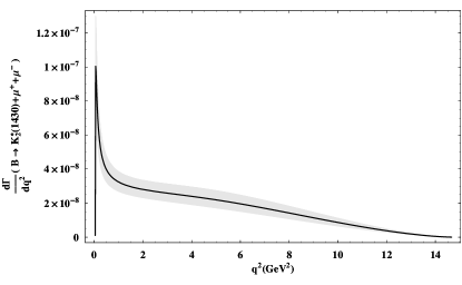
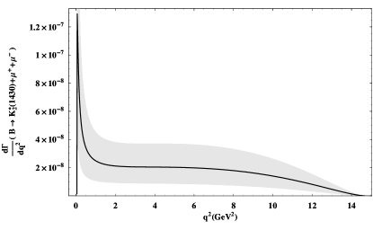
Figure 1: The shaded region show the uncertainty in the branching ratio of $B\to K_{2}^{\ast}(1430)l^{+}l^{-}$ calculation in (a) LCSR form factors and (b) pQCD form factors.

In order to make the quantitative analysis we have used the following values of the input parameters: $\alpha_{s}(m_{Z})=0.118$, $\alpha_{s}(m_{b})=0.223$, $m_{W}=80.22$GeV, $m_{b}=4.19$ GeV, $m_{c}=1.27$ GeV, $\tau_{B}=1.55\times 10^{-12}$sec, $f_{B}=200$ MeV and $m_{B}=5.28$ GeV, respectively. As in the exclusive $B$ meson decays the main inputs are the form factors which are non-perturbative quantities and one needs some model to calculate them. In order to make a reliable NP study one has to control the uncertainties arising from the different input parameters where form factors are the major contributors. The values of form factors calculated in pQCD approach Wei and in LCSR approach LCSR are summarized in Tables I and II respectively.

Using above given inputs along with the numerical values of the form factors calculated in LCSR(pQCD) approach (c.f. Tables I and II) the values of branching ratios for $B\rightarrow K_{2}^{\ast}(1430)l^{+}l^{-}(l=\mu,\tau)$ in SM are found to be Wei

$$Br(B\rightarrow K_{2}^{\ast}(1430)\mu^{+}\mu^{-})=2.43{{}^{+0.6}_{-0.5}}(2.5{{}^{+1.6}_{-1.1}})\times 10^{-7},$$

$$Br(B\rightarrow K_{2}^{\ast}(1430)\tau^{+}\tau^{-})=2.74{{}^{+0.9}_{-0.9}}(9.6{{}^{+6.2}_{-4.5}})\times 10^{-10}.$$ (49)

which is sizable and is well within the range of the LHCb. Also due to the similarity between this and its brother $B\rightarrow K^{*}(892)l^{+}l^{-}$ decay all the experimental techniques for well studied $B\rightarrow K^{*}(892)l^{+}l^{-}$ decays will be easily adjustable to $B\rightarrow K_{2}^{\ast}(1430)l^{+}l^{-}$ decays. The main decay of $K^{\ast}_{2}(1430)$ is the charged kaon and pion which are detectable at the LHCb Wei .

Here we can see that compared to the pQCD the LCSR uncertainties are much smaller as seen in Table I and II. In Figs. 1 we have displayed the branching ratios of $B\rightarrow K_{2}^{\ast}(1430)\mu^{+}\mu^{-}$ decays along with the error bands. It can be seen that in case of pQCD form factors the uncertainty region is much wider compared to that of LCSR form factors. Therefore, in the forthcoming analysis of $B\rightarrow K_{2}^{\ast}(1430)l^{+}l^{-}(l=\mu,\tau)$ in the SM4 we will use the LCSR form factors.

Now to study the complementarity of the $B\rightarrow K_{2}^{\ast}(1430)l^{+}l^{-}$ and $B\rightarrow K^{\ast}(892)l^{+}l^{-}$ we have also incorporated in this numerical study the results of the SM4 on the decays $B\rightarrow K^{\ast}(892)l^{+}l^{-}(l=\mu,\tau)$. For this process $B\rightarrow K^{\ast}(892)l^{+}l^{-}(l=\mu,\tau)$ we have used the LCSR form factors calculated by A. Ali et. al. Ali-ball . The plots for both decay channels with final state mesons $K_{2}^{*}$ and $K^{*}$ are presented side by side for each observable in this phenomenological analysis.

Regarding the parameters of the SM4, recently CDF collaboration has given the lower bound on the mass of the $t^{\prime}$ quark to be $m_{t^{\prime}}\geq 335$ GeV at $95\%$ CL CDFNEW . These bounds are little higher than the ones quoted in Ref. CDF of $m_{t^{\prime}}\gtrsim 256$ GeV. On the other hand, the perturbativity of the Yukawa coupling implies that $m_{t}^{\prime}\lesssim\sqrt{2\pi}\left\langle v\right\rangle\approx 600$ GeV, where $\left\langle v\right\rangle$ is the vacuum expectation value of the Higgs boson Londonnewsm4 . Thus, the mass $m_{t}^{\prime}$ is constrained in a band, $m_{t^{\prime}}=335-600$ GeV, which increases the predictability of SM4. Keeping in view that these bounds will be considerably improved at LHC, we will consider $m_{t^{\prime}}=300-600$ GeV in our numerical calculation. In addition to the masses of the sequential fourth generation of quarks the other important parameters are the CKM4 matrix elements, where $|V_{t^{\prime}s}|$ and $|V_{t^{\prime}b}|$ are of the main interest for present study. The experimental upper bounds on these CKM matrix elements are $|V_{t^{\prime}s}|<0.11$ and $|V_{t^{\prime}b}|<0.12$ boundsCKM ; Samitra . By taking the CKM unitarity condition, $\sum\limits_{i}V_{is}^{\ast}V_{ib},~{}(i=u,c,t,t^{\prime})$ together with the present measurements of the $3\times 3$ CKM matrix boundsSM3 , the bounds for CKM4 matrix elements are obtained to be boundsSM4 ; Samitra

$$|V_{t^{\prime}s}^{\ast}V_{t^{\prime}b}|\leq 1.2\times 10^{-2}.$$ (50)

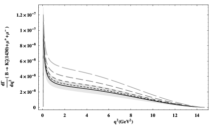
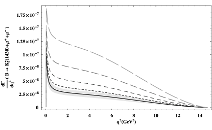
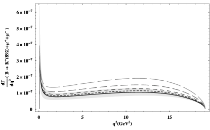
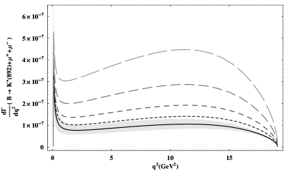
Figure 2: The dependence of decay rate of $B\rightarrow K_{2}^{\ast}(1430)\mu^{+}\mu^{-}$ on $q^{2}$ and $B\rightarrow K^{\ast}(892)\mu^{+}\mu^{-}$ for different values of $m_{t^{\prime}}$ and $\left|V_{t^{\prime}b}^{\ast}V_{t^{\prime}s}\right|$. $\left|V_{t^{\prime}b}^{\ast}V_{t^{\prime}s}\right|$ $=$ $0.006$ and $0.012$ in (a,b) and (c,d) respectively. In all the graphs, the solid line corresponds to the SM, dotted line, dashed, medium dashed and long dashed lines are for $m_{t^{\prime}}$ $=$ $300$ GeV and $400$ GeV, $500$ GeV and $600$ GeV respectively. Shaded region reflects the uncertainties involved in different input parameters.

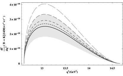
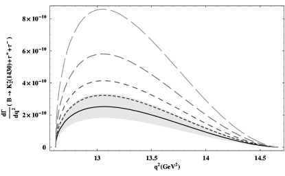
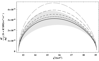
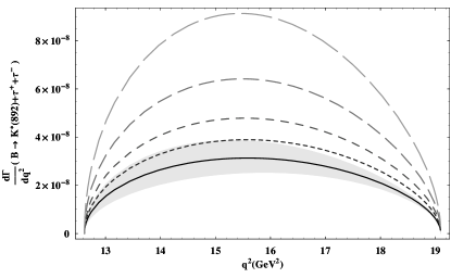
Figure 3: The dependence of decay rate of $B\rightarrow K_{2}^{\ast}(1430)\tau^{+}\tau^{-}$ and $B\rightarrow K^{\ast}(892)\tau^{+}\tau^{-}$ on $q^{2}$ for different values of $m_{t^{\prime}}$ and $\left|V_{t^{\prime}b}^{\ast}V_{t^{\prime}s}\right|$. $\left|V_{t^{\prime}b}^{\ast}V_{t^{\prime}s}\right|$ $=$ $0.006$ and $0.012$ in (a,b) and (c,d) respectively. In all the graphs, the solid line corresponds to the SM, dotted line, dashed, medium dashed and long dashed lines are for $m_{t^{\prime}}$ $=$ $300$ GeV and $400$ GeV, $500$ GeV and $600$ GeV respectively.

The numerical results for the branching ratios, forward-backward asymmetry, different polarization asymmetries of final state lepton and the helicity fractions of final state meson in $B\to(K^{\ast}_{2},K^{*})l^{+}l^{-}$ decays are depicted in Figs. 2-12. Fig. 2(a,b) describes the differential branching ratio of $B\rightarrow K_{2}^{\ast}(1430)\mu^{+}\mu^{-}$ decay, where one can see that the fourth generation effects are quite distinctive from those of the SM results both in the small and large momentum transfer $(q^{2})$ region. At small value of $q^{2}$ the dominant contribution comes from $C_{7}^{tot}(\mu)$ whereas for the large value of $q^{2}$ the major contribution is from the $Z$ exchange i.e., $C_{10}^{tot}$, which is sensitive to the mass of the fourth generation quark $m_{t^{\prime}}$. Now for the final state dimuon case, we can see that the differential branching ratio is enhanced sizable in terms of $m_{t^{\prime}}$ and $\left|V_{t^{\prime}b}^{\ast}V_{t^{\prime}s}\right|$. It is clear from Table III that for $m_{t^{\prime}}=600$ and $\left|V_{t^{\prime}b}^{\ast}V_{t^{\prime}s}\right|=1.2\times 10^{-2}$ the branching ratio of $B\rightarrow K_{2}^{\ast}(1430)\mu^{+}\mu^{-}$ decay is increased by a factor of $4$ in magnitude. Similar effects can also be observed for $B\rightarrow K_{2}^{\ast}(1430)\tau^{+}\tau^{-}$ decay presented in Fig. 3(a,b).

To compare the phenomenological profile of $B\to K_{2}^{\ast}(1430)l^{+}l^{-}$ and $B\to K^{\ast}(892)l^{+}l^{-}$ decays, we have taken the effects of the SM4 on the decays $B\rightarrow K^{\ast}(892)l^{+}l^{-}$, $l=\mu,\tau$ as well. The branching ratios for these decays are shown in Figs. 2(c,d) and 3(c,d) for the final state leptons are muons and tauons, respectively. Though the branching ratio of $B\rightarrow K_{2}^{\ast}(1430)\mu^{+}\mu^{-}$ is approximately $8$ times smaller in magnitude than the value of $B\rightarrow K^{\ast}(892)\mu^{+}\mu^{-}$ decay calculated in Ali-ball , but the SM4 contributions are almost same. Therefore, the phenomenology of $B\rightarrow K_{2}^{\ast}(1430)l^{+}l^{-}$ decay is as rich as it’s brother decay $B\rightarrow K^{\ast}(892)l^{+}l^{-}$.

Table 3: Branching ratio for $B\to K_{2}^{\ast}(1430)\mu^{+}\mu^{-}(\tau^{+}\tau^{-})$ decay for different values of $m_{t^{\prime}}$ and $\left|V_{t^{\prime}b}^{\ast}V_{t^{\prime}s}\right|$.

$m_{t^{\prime}}\left(\text{GeV}\right)$	$\left|V_{t^{\prime}b}V_{t^{\prime}s}\right|=3\times 10^{-3}$	$\left|V_{t^{\prime}b}V_{t^{\prime}s}\right|=6\times 10^{-3}$	$\left|V_{t^{\prime}b}V_{t^{\prime}s}\right|=9\times 10^{-3}$	$\left|V_{t^{\prime}b}V_{t^{\prime}s}\right|=12\times 10^{-3}$
$300$	$2.59\times 10^{-7}\left(6.56\times 10^{-10}\right)$	$2.74\times 10^{-7}\left(6.82\times 10^{-10}\right)$	$3.00\times 10^{-7}\left(7.27\times 10^{-10}\right)$	$3.34\times 10^{-7}\left(7.90\times 10^{-10}\right)$
$400$	$2.66\times 10^{-7}\left(6.65\times 10^{-10}\right)$	$3.02\times 10^{-7}\left(7.21\times 10^{-10}\right)$	$3.62\times 10^{-7}\left(8.14\times 10^{-10}\right)$	$4.47\times 10^{-7}\left(9.45\times 10^{-10}\right)$
$500$	$2.79\times 10^{-7}\left(6.82\times 10^{-10}\right)$	$3.55\times 10^{-7}\left(7.91\times 10^{-10}\right)$	$4.81\times 10^{-7}\left(9.72\times 10^{-10}\right)$	$6.58\times 10^{-7}\left(1.22\times 10^{-10}\right)$
$600$	$3.01\times 10^{-7}\left(7.11\times 10^{-10}\right)$	$4.43\times 10^{-7}\left(9.06\times 10^{-10}\right)$	$6.80\times 10^{-7}\left(1.23\times 10^{-9}\right)$	$1.01\times 10^{-6}\left(1.69\times 10^{-9}\right)$

In order to make the analysis more predictive the sensitivity of the branching ratio of $B\to K_{2}^{\ast}(1430)l^{+}l^{-}$ (after integration on $q^{2}$) on the fourth generation parameters is presented in Figs. 4 and 5 for final state leptons as $\mu$ and $\tau$, respectively. We can see that the NP effects arising due to the SM4 parameters are significantly different from that of the SM results.

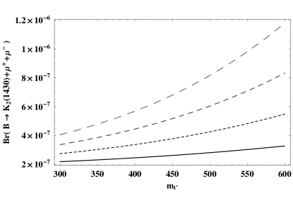
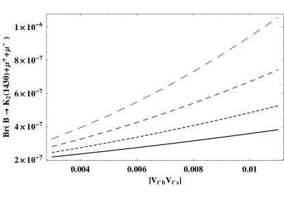
Figure 4: (a)The Dependence of Decay Width of $B\rightarrow K_{2}^{\ast}(1430)\mu^{+}\mu^{-}$ on $m_{t^{\prime}}$ for values of $\left|V_{t^{\prime}b}^{\ast}V_{t^{\prime}s}\right|$ = $3\times 10^{-3}$, $6\times 10^{-3}$, $9\times 10^{-3}$, $1.2\times 10^{-2}$, $1.5\times 10^{-2}$. (b) The Dependence of Decay Width on $\left|V_{t^{\prime}b}^{\ast}V_{t^{\prime}s}\right|$ for values of $m_{t^{\prime}}$ = $300$ GeV, $400$ GeV, $500$ GeV, $600$ GeV. The legends are same as in Fig. 2.

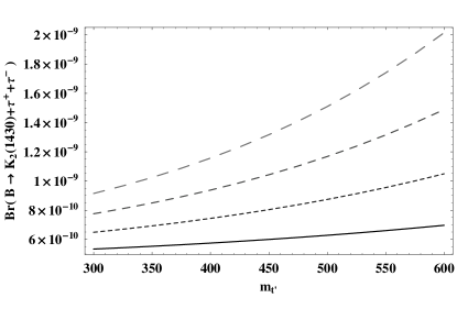
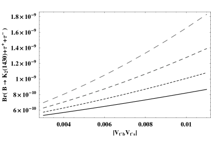
Figure 5: (a) The Dependence of Decay Width of $B\rightarrow K_{2}^{\ast}(1430)\tau^{+}\tau^{-}$ on $m_{t^{\prime}}$ for values of $\left|V_{t^{\prime}b}^{\ast}V_{t^{\prime}s}\right|$ = $3\times 10^{-3}$, $6\times 10^{-3}$, $9\times 10^{-3}$, $1.2\times 10^{-2}$, $1.5\times 10^{-2}$. (b) The Dependence of Decay Width on $\left|V_{t^{\prime}b}^{\ast}V_{t^{\prime}s}\right|$ for values of $m_{t^{\prime}}$ = $300$ GeV, $400$ GeV, $500$ GeV, $600$ GeV. The legends are same as in Fig. 2.

As an exclusive decay, there are different sources of uncertainties involved in the calculation of the above decay. The major uncertainties in the numerical analysis of $B\rightarrow K_{2}^{\ast}(1430)l^{+}l^{-}$ decay originate from the $B\rightarrow K_{2}^{\ast}(1430)$ transition form factors calculated in the LCSR approach, as shown in Table II, can bring about $20-30\%$ errors to the differential branching ratios. This shows that it may not be a suitable tool to look for the new physics for small values of the SM4 parameters. This can also be seen from Fig. 2a where for small values of SM4 parameters the NP effects lies inside the uncertainty band. Therefore, we have to look for the observables where hadronic uncertainties almost have no effect. Among them the most alluring are the zero position of the forward-backward asymmetry, lepton polarization asymmetries and the helicity fractions of the final state meson, which being almost free from the hadronic uncertainties, serve as an important tool to look for the NP.

In the SM the zero crossing of the FBA is due to the destructive interference between the photon penguin ($C_{7}^{eff}$) and the $Z$ penguin ($C_{9}^{eff}$) and at the leading order in $\alpha_{s}$ this is independent of the form factors. For the decay $B\rightarrow K_{2}^{\ast}(1430)\mu^{+}\mu^{-}$, the value of the the zero crossing is approximately $(q^{2}\simeq 4.0\text{GeV}^{2})$. The deviation of the zero crossing from the SM value gives us some clues for the NP. Fig. 6 (a,b) shows the effect of the fourth generation on the zero-position of the forward-backward asymmetry for $B\rightarrow K_{2}^{\ast}(1430)\mu^{+}\mu^{-}$. One can see that the value of the forward-backward asymmetry decreases from the SM value but the position of zero crossing remains the same for the low value of SM4 parameters $(m_{t^{\prime}},\left|V_{t^{\prime}b}^{\ast}V_{t^{\prime}s}\right|)$ (c.f. Fig. 6(a,b)). However at the large value of the CKM4 matrix elements and the mass $m_{t^{\prime}}$ the zero position is shifted to the For $B\rightarrow K_{2}^{\ast}(1430)\tau^{+}\tau^{-}$ the forward-backward asymmetry is presented in Fig. 7(a,b). Here, one can easily distinguish the SM4 from that of the SM. For the decay $B\rightarrow K^{\ast}(892)l^{+}l^{-}$ Figs. 6,7(c,d) show similar pattern but with different value of FBA zero crossing. Thus the forward backward asymmetry qualitatively show that the two decays, as expected, are very much alike.

Here we would like to make an important remark: It has been shown by Beneke et. al. that next-to-leading (NLO) corrections to $B\to K^{\ast}(892)l^{+}l^{-}$ decays give small corrections to the invariant mass spectrum, but there is a large correction to the predicted location of the forward-backward asymmetry zero Beneke which is about $30\%$. This is because of the fact that all dependence of the form factors arises first at NLO. Therefore, to perform a reliable NP study in the zero position of the forward-backward asymmetry one needs such kind of calculation for $B\to K_{2}^{\ast}(1430)l^{+}l^{-}$ decay process as well.

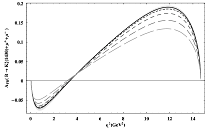
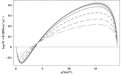
Figure 6: The dependence of forward-backward asymmetry of $B\rightarrow K_{2}^{\ast}(1430)\mu^{+}\mu^{-}$ and $B\rightarrow K^{\ast}(892)\mu^{+}\mu^{-}$ on $q^{2}$ for different values of $m_{t^{\prime}}$ and $\left|V_{t^{\prime}b}^{\ast}V_{t^{\prime}s}\right|$ in (a,b) and (c,d) respectively. The values of the fourth generation parameters and the legends are same as in Fig. 2.

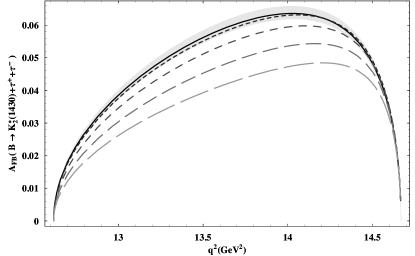
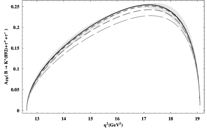
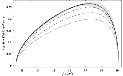
Figure 7: The dependence of forward-backward asymmetry of $B\rightarrow K_{2}^{\ast}(1430)\tau^{+}\tau^{-}$ and $B\rightarrow K^{\ast}(892)\tau^{+}\tau^{-}$ on $q^{2}$ for different values of $m_{t^{\prime}}$ and $\left|V_{t^{\prime}b}^{\ast}V_{t^{\prime}s}\right|$ in (a,b) and (c,d) respectively. The values of the fourth generation parameters and the legends are same as in Fig. 2.

Fig. 8(a,b) shows the dependence of longitudinal lepton polarization asymmetry for the $B\rightarrow K_{2}^{\ast}(1430)\mu^{+}\mu^{-}$ decay on the square of momentum transfer for different values of $m_{t^{\prime}}$ and $\left|V_{t^{\prime}b}^{\ast}V_{t^{\prime}s}\right|$. The value of longitudinal lepton polarization for muon is around $1$ in the SM and we have significant deviation in this value in the SM4. Just in the case of $m_{t^{\prime}}=600$ GeV and $\left|V_{t^{\prime}b}^{\ast}V_{t^{\prime}s}\right|=1.2\times 10^{-2}$ the value of the longitudinal lepton polarization becomes $0.4$ which will help us to see experimentally the SM4 effects in these decays. Similar effects can been seen for the final state tauon (c.f. Fig. 8(c,d)). In this case the shift from the SM value is very small because of the factor $\left(1-\frac{4m_{l}^{2}}{q^{2}}\right)$ in Eq. (42). Following the same lines the longitudinal lepton polarization asymmetry for $B\rightarrow K^{\ast}(892)l^{+}l^{-}$ is shown in Fig 8(e,f,g,h). Here we can see that the longitudinal lepton polarization asymmetry for $B\rightarrow K^{\ast}(892)l^{+}l^{-}$ go hand in hand with its predecessor tensor decay $B\rightarrow K_{2}^{\ast}(1430)l^{+}l^{-}$.

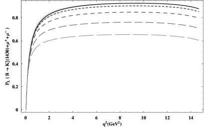
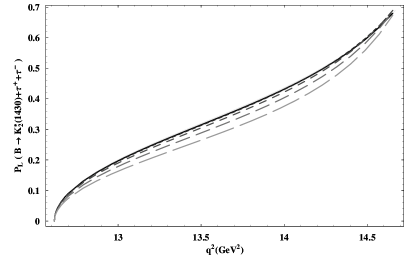
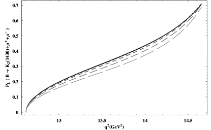
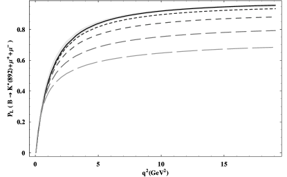
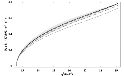
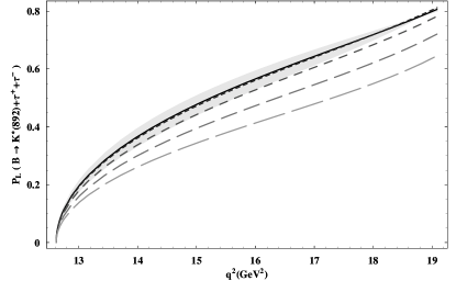
Figure 8: The dependence of longitudinal lepton polarization asymmetry of $B\rightarrow K_{2}^{\ast}(1430)l^{+}l^{-}(l=\mu,\tau)$ and $B\rightarrow K^{\ast}(892)l^{+}l^{-}$ on $q^{2}$ for different values of $m_{t^{\prime}}$ and $\left|V_{t^{\prime}b}^{\ast}V_{t^{\prime}s}\right|$. The values of the fourth generation parameters and the legends are same as in Fig. 2.

The dependence of normal lepton polarization asymmetries for $B\rightarrow K_{2}^{\ast}l^{+}l^{-}$ on the momentum transfer square are presented in Fig. 9(a,b,c,d). In terms of Eq. (43), one can see that it is proportional to the mass of the final state lepton. In the SM4 one can see a slight shift, from the SM value, which is not so large for $l=\mu$ as from Eq. (43). Now for $l=\tau$ one expects large values of normal lepton polarization compared to the $l=\mu$ case. Figure 9(c,d) shows that there is a significant increase in the value of $P_{N}$ in the SM4 parameter space. As for $B\rightarrow K^{\ast}(892)l^{+}l^{-}$ decay, $P_{N}$ of $K^{\ast}$is distinctively different $P_{N}$ of $K_{2}^{\ast}$in low $q^{2}$ region for final state muons (Fig. 9(e,f)). While for the tauons the $P_{N}(K^{*})$ looks altogether different from $P_{N}(K_{2}^{*})$ as depicted in Fig. 9(g,h). Even for the extreme values of the SM4 parameters effects on the $P_{N}(K^{\ast})$ falls inside the error bands, which is not the case for $P_{N}(K_{2}^{\ast})$ (c.f. Fig. 9(d,h)). Thus SM4 effects on $P_{N}$ can distinguish very clearly between of these two semileptonic decay channels.

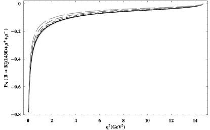
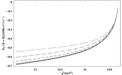
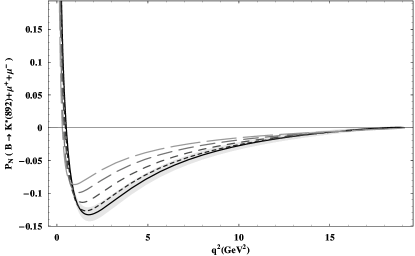
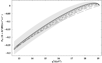
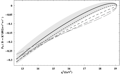
Figure 9: The dependence of Normal lepton polarization asymmetry of $B\rightarrow K_{2}^{\ast}(1430)l^{+}l^{-}(l=\mu,\tau)$ and $B\rightarrow K^{\ast}(892)l^{+}l^{-}$ on $q^{2}$ for different values of $m_{t^{\prime}}$ and $\left|V_{t^{\prime}b}^{\ast}V_{t^{\prime}s}\right|$. The values of the fourth generation parameters and the legends are same as in Fig. 2.

Fig. 10 show the value of transverse lepton polarization both in the SM as well as in the SM4 for $B\rightarrow K_{2}^{\ast}(1430)l^{+}l^{-}$ and $B\rightarrow K_{2}^{\ast}(892)l^{+}l^{-}$ decays. It is clear that it is zero in the SM but non zero in the sequential fourth generation SM (SM4). This non zero value comes from the interference of the Wilson coefficient for SM4 which are complex in SM4, see Eqs. (16, 17). If we compare the two decays involving $K^{*}(892)$ and $K_{2}^{*}(1430)$ the transverse lepton polarization look almost identical (c.f. Fig. 10(a,b,c,d)). The transverse lepton polarization is proportional to the lepton mass which makes its value small for the muons, ane for the tauons (Fig. 10(e,f,g,h)) the value of the transverse lepton polarization is slightly larger.

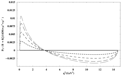
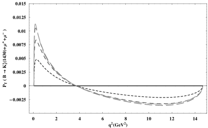
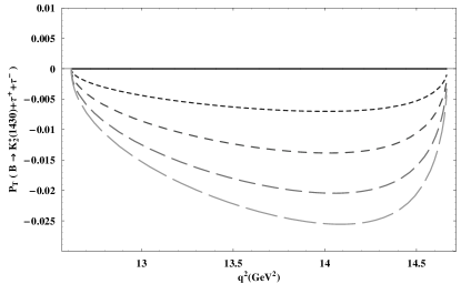
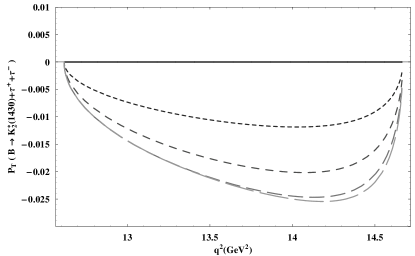
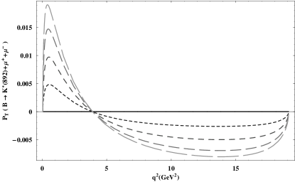
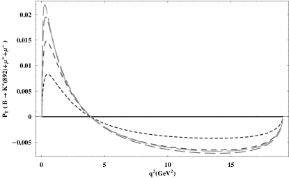
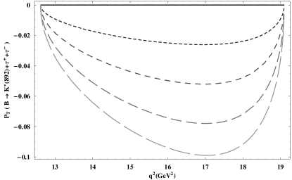
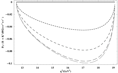
Figure 10: The dependence of Transverse lepton polarization asymmetry of $B\rightarrow K_{2}^{\ast}(1430)l^{+}l^{-}(l=\mu,\tau)$ and $B\rightarrow K^{\ast}(892)l^{+}l^{-}$ on $q^{2}$ for different values of $m_{t^{\prime}}$ and $\left|V_{t^{\prime}b}^{\ast}V_{t^{\prime}s}\right|$. The values of the fourth generation parameters and the legends are same as in Fig. 2.

In order to study the spin structure of the out going meson, the helicity fractions act as an ideal probe. Since $K_{2}^{*}(1430)$ is a tensor particle therefore its spin structure is very different from its corresponding ground state vector meson $K^{*}(890)$. Figure 11 shows longitudinal helicity fraction of both decays involving $K_{2}^{*}(1430)$ and $K^{*}(892)$. It can be clearly seen that the longitudinal helicity fraction for these two decays have different signatures especially in case of $l=\mu$. The longitudinal helicity fraction $f_{L}(K_{2}^{*}(1430))$ with $l=\mu$ starts with initial values of $0.8$ and then the values drop down the hill to about $0.4$ at high $q^{2}$. On the other hand for $K^{*}(892)$ the longitudinal helicity fraction begins with higher value of about $0.9$ and ends at lower value of $0.3$. However, when the final state lepton is $\tau$ the new physics effects become more prominent in both decays. The $f_{L}$ values for decays involving $K_{2}^{*}(1430)$ and $K^{*}(892)$ as final state mesons numerically begin with $0.75$ and $0.62$ respectively and finish at $0.4$ and $0.3$ respectively (Figs 11(c,d,g,h)). This difference between the initial values and the final values of $f_{L}$, for the to decay modes, show that these decays are behaving differently from each other when we study the spin effects of the final state meson.

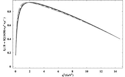
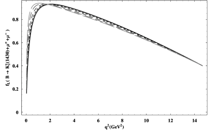
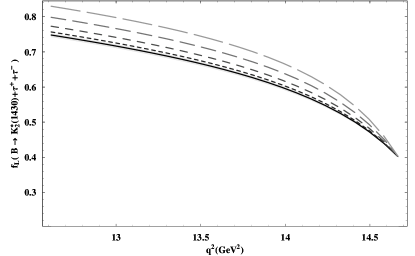
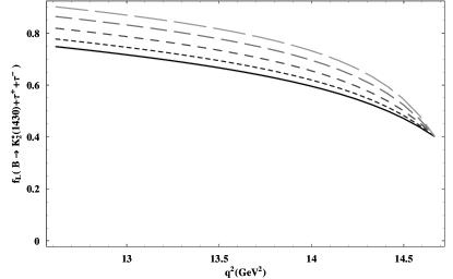
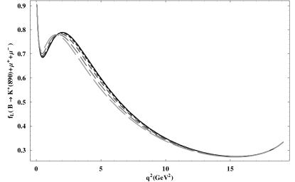
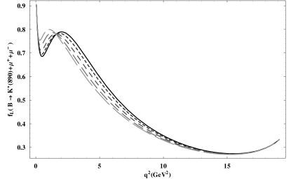
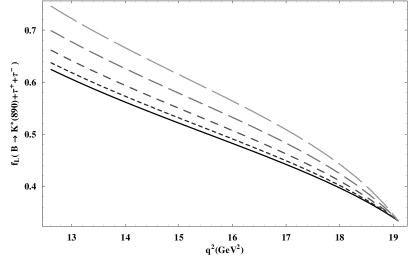
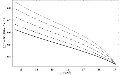
Figure 11: The dependence of Longitudinal helicity fraction of $B\rightarrow K_{2}^{\ast}(1430)l^{+}l^{-}$ and $B\rightarrow K^{\ast}(892)l^{+}l^{-}$ on $q^{2}$ for different values of $m_{t^{\prime}}$ and $\left|V_{t^{\prime}b}^{\ast}V_{t^{\prime}s}\right|$. The values of the fourth generation parameters and the legends are same as in Fig. 2.

The transverse helicity fractions of final state meson behave contrary to longitudinal helicity fraction since helicity fractions add up to give unity (c.f. Fig. 12). A significant shift in the SM4 from the corresponding SM value is found in the transverse helicity fractions both for the $K^{\ast}(892)$ and $K_{2}^{\ast}(1430)$ mesons.

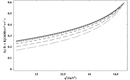
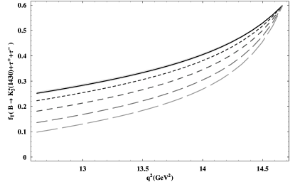
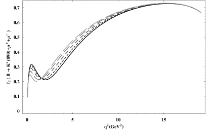
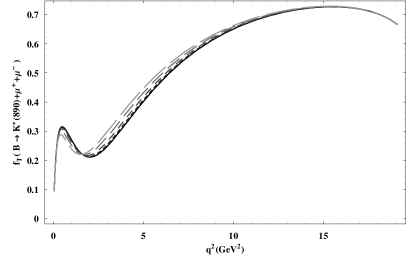
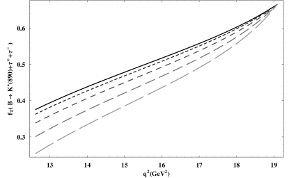
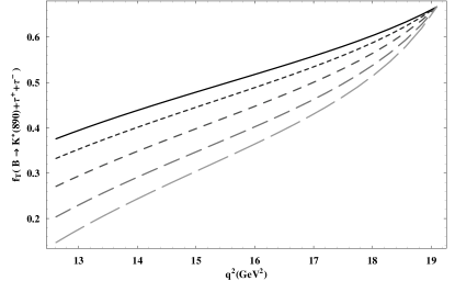
Figure 12: The dependence of Transverse helicity fraction of $B\rightarrow K_{2}^{\ast}(1430)l^{+}l^{-}$ on $q^{2}$ for different values of $m_{t^{\prime}}$ and $\left|V_{t^{\prime}b}^{\ast}V_{t^{\prime}s}\right|$. The values of the fourth generation parameters and the legends are same as in Fig. 2.

VI Conclusion:

We have carried out the study of invariant mass spectrum, forward-backward asymmetry, lepton polarization asymmetries and the helicity fractions of the final state meson $(K_{2}^{\ast})$ for the semileptonic decay $B\rightarrow K_{2}^{\ast}(1430)l^{+}l^{-}$ $(l=\mu,\tau)$ in SM4. In particular, we have analyzed the sensitivity of these physical observables on the fourth generation quark mass $m_{t^{\prime}}$ as well as the CKM mixing angle $\left|V_{t^{\prime}b}^{\ast}V_{t^{\prime}s}\right|$. We have also made a qualitative analysis between $B\rightarrow K_{2}^{\ast}(1430)l^{+}l^{-}$ and the corresponding $B\rightarrow K^{\ast}(892)l^{+}l^{-}$ decays. The main outcomes of this study can be summarized as follows:

• The differential branching ratios deviate sizably from that of the SM especially both in the small and large momentum transfer region. These effects are significant and the branching ratio increases by a factor of $4$ for $m_{t^{\prime}}$ $=$ $600$ GeV and $\left|V_{t^{\prime}b}^{\ast}V_{t^{\prime}s}\right|$ $=$ $1.2\times 10^{-2}$ in $B\rightarrow K_{2}^{\ast}(1430)\mu^{+}\mu^{-}$ decay. Though the branching ratio of this decay is an order of magnitude smaller than its brother decay $B\rightarrow K^{\ast}(892)l^{+}l^{-}$ but the SM4 effects in both the decays are same. Now for the final state tauon’s case, the increases in the value of the branching ratio of $B\rightarrow K_{2}^{\ast}(1430)\tau^{+}\tau^{-}$ decay is very small and is usually masked by the uncertainties involved in different input parameters like form factors.

• The value of the forward-backward asymmetry decreases significantly from that of the SM value in the SM4 when the mass of the fourth generation quark varies from $300$ GeV to $600$ GeV. The value of the zero position of forward-backward asymmetry shifted towards the left for all values of $\left|V_{t^{\prime}b}^{\ast}V_{t^{\prime}s}\right|$ in $B\rightarrow K_{2}^{\ast}(1430)\mu^{+}\mu^{-}$ decay. This shifting is significant for large values of the fourth generation CKM matrix elements $\left|V_{t^{\prime}b}^{\ast}V_{t^{\prime}s}\right|$ and fourth generation top quark mass $m_{t^{\prime}}$. It is known that the NLO corrections to $B\to K^{\ast}l^{+}l^{-}$ decay can bring $30\%$ corrections to the zero position of the FBA, therefore, such calculation for $B\to K_{2}^{\ast}(1430)l^{+}l^{-}$ is still lacking.

• The longitudinal, normal and transverse polarizations of leptons are calculated in the SM4. We observed that the longitudinal and transverse lepton polarization asymmetry in $B\to K_{2}^{\ast}(1430)l^{+}l^{-}$ and $B\to K^{\ast}(892)l^{+}l^{-}$ decays are same but the normal lepton polarization of these two decays is different. It is found that the SM4 effects are very promising in both decays, which could be measured at future experiments, and would shed light on the new physics beyond the SM. It is hoped that this can be measurable at the LHCb where a large number of $\ b\bar{b}$ pairs are expected to be produced.

• The SM4 effects on helicity fraction are mild but still notably different from SM. In case of $B\to K_{2}^{\ast}\tau^{+}\tau^{-}$ the asymptotic values of $f_{L}$ and $f_{T}$ are distinctly different from their SM values. This observable is also important to probe NP effects on the final state tensor meson $K_{2}^{*}$ and vector meson $K^{*}$. A comparison of the helicity fractions of $K_{2}^{\ast}(1430)$ and $K^{\ast}(892)$ was also investigated and it was found that both decay modes are not entirely similar in all respects.

In summary, the experimental investigation of observables, like branching ratios, forward-backward asymmetry, lepton polarization asymmetries and the helicity fractions of the final state $K_{2}^{\ast}(1430)$ meson in $B\rightarrow K_{2}^{\ast}(1430)l^{+}l^{-}$ decay will be a useful compliment of the much investigated $B\rightarrow K^{\ast}(892)l^{+}l^{-}$ decay.

References

- (1) A. Ali, P. Ball, L. T. Handoko et al., Phys. Rev. D61, 074024 (2000). [hep-ph/9910221]; C. S. Kim, Y. G. Kim, C. D. Lu and T. Morozumi, Phys. Rev. D62, 034013 (2000) [arXiv:hep-ph/0001151]; M. Beneke, T. Feldmann, D. Seidel, Nucl. Phys. B612, 25-58 (2001). [hep-ph/0106067]; C. H. Chen and C. Q. Geng, Nucl. Phys. B636, 338 (2002) [arXiv:hep-ph/0203003]; F. Kruger and J. Matias, Phys. Rev. D71, 094009 (2005) [arXiv:hep-ph/0502060]; A. Ali, G. Kramer, G. -h. Zhu, Eur. Phys. J. C47, 625-641 (2006). [hep-ph/0601034]; C. Bobeth, G. Hiller and G. Piranishvili, JHEP 0807, 106 (2008) [arXiv:0805.2525 [hep-ph]]; U. Egede, T. Hurth, J. Matias, M. Ramon and W. Reece, JHEP 0811, 032 (2008) [arXiv:0807.2589 [hep-ph]]; W. Altmannshofer, et al., JHEP 0901, 019 (2009). [arXiv:0811.1214 [hep-ph]]; C. W. Chiang, R. H. Li and C. D. Lu, arXiv:0911.2399 [hep-ph]; A. K. Alok, A. Dighe, D. Ghosh, D. London, J. Matias, M. Nagashima and A. Szynkman, JHEP 1002, 053 (2010) [arXiv:0912.1382 [hep-ph]]; Q. Chang, X. Q. Li and Y. D. Yang, JHEP 1004, 052 (2010) [arXiv:1002.2758 [hep-ph]]; A. Bharucha and W. Reece, Eur. Phys. J. C69, 623 (2010) [arXiv:1002.4310 [hep-ph]]; A. Khodjamirian, T. Mannel, A. A. Pivovarov and Y. M. Wang, JHEP 1009, 089 (2010) [arXiv:1006.4945 [hep-ph]]; C. Bobeth, G. Hiller and D. van Dyk, JHEP 1007, 098 (2010) [arXiv:1006.5013 [hep-ph]]; A. K. Alok, A. Datta, A. Dighe, M. Duraisamy, D. Ghosh, D. London and S. U. Sankar, arXiv:1008.2367 [hep-ph].
- (2) B. Aubert et al. [BABAR Collaboration], Phys. Rev. Lett. 102, 091803 (2009) [arXiv:0807.4119 [hep-ex]]; J. T. Wei et al. [BELLE Collaboration], Phys. Rev. Lett. 103, 171801 (2009) [arXiv:0904.0770 [hep-ex]]; T. Aaltonen et al. [CDF Collaboration], Phys. Rev. D79, 011104 (2009) [arXiv:0804.3908 [hep-ex]].
- (3) B. Adeva, et al. [LHCb Collaboration], arXiv:0912.4179 [hep-ex]; M. Patel and H. Skottowe, A Fisher discriminant selection for at LHCb, LHCb-2009-009.
- (4) R. L. Gac, [LHCb Collaboration], arXiv:1009.5902 [hep-ex].
- (5) B. Aubert et al. [BABAR Collaboration], Phys. Rev. D70, 091105 (2004) [arXiv:hep- ex/0409035]; S. Nishida et al. [Belle Collaboration], Phys. Rev. Lett. 89, 231801 (2002) [arXiv:hep-ex/0205025].
- (6) S. Rai Choudhury, et al., Phys. Rev. D74, 054031 (2006) [hep-ph/0607289]; S. R. Choudhury, A. S. Cornell and N. Gaur, Phys. Rev. D81, 094018 (2010) [arXiv:0911.4783 [hep-ph]]; H. Hatanaka and K. C. Yang, Phys. Rev. D79, 114008 (2009) [arXiv:0903.1917 [hep-ph]]; H. Hatanaka and K. C. Yang, Eur. Phys. J. C67, 149 (2010), arXiv:0907.1496 [hep-ph].
- (7) W. Wang, Phys. Rev. D83, 014008 (2011) arXiv: 1008.5326 [hep-ph]; Run-Hui Li, Cai-Dian Lu and Wei Wang, arXiv: 1012.2129 [hep-ph]
- (8) B. Holdom, W. -S. Hou, T. Hurth, M. L. Mangano, S. Sultansoy and G. Unel, PMC Phys. A3 (2009) 4.
- (9) W. -S. Hou, A. Soni and H. Steger, Phys. Lett. B192(1987) 441; W. S. Hou, R. S. Willey and A. Soni, Phys. Rev. Lett. 58 (1987) 1358;
- (10) M. Chanowitz, Phys. Lett. B352 (1995) 376.
- (11) M. Hashimoto, arXiv:1001.4335; J. Alwall et al., Eur. Phys. J. C49 (2007) 791-801, hep-ph/0607115; M. S. Chanowitz, Phys. Rev. D79 (2009) 113008, arXiv: 0904.3570; V. A. Novikov, A. N. Rozanov, and M. I. Vysotsky, arXiv: 0904.4570; J. Erler and P. Langacker, arXiv: 1003.3211; H.-J. He, N. Polonsky, S. Su, Phys. Rev. D64 (2001) 053004, [hep-ph/0102144]; P. Q. Hung and C. Xiong, arXiv: 0911.3890; P. Q. Hung and C. Xiong, arXiv: 0911.3892; K. S. Babu, X. G. He, X. Li, and S. Pakvasa, Phys. Lett. B205 (1988) 540; D. London, Phys. Lett. B234 (1990) 354; Y. Dincer, Phys. Lett. B505 (2001) 89; A. Arhrib and W.-S. Hou, Eur. Phys. J. C27 (2003) 555-561, hep-ph/0211267; W.-S. Hou, M. Nagashima, and A. Soddu, Phys. Rev. D72 (2005) 115007, hep-ph/0508237; W.-S. Hou, M. Nagashima, and A. Soddu, Phys. Rev. D76 (2007) 013504, hep-ph/0610385; T. M. Aliev, A. Ozpineci and M. Savci, Nucl. Phys. B585 (2000) 275. T. M. Aliev, A. Ozpineci and M. Savci, Eur. Phys. J. C29 (2003) 265; V. Bashiry and K. Azizi, JHEP 0707 (2007) 64; V. Bashiry and F. Flahati, arXiv: 0707.3242; F. Zolfagharpour and V. Bashiry, arXiv: 0707.4337; V. Bashiry and M. Bayer, arXiv: 0903.2631; A. Soni, A. K. Alok, A. Giri, R. Mohanta, and S. Nandi, arXiv: 0807.1971; J. A. Herrera, R. H. Benavides, and W. A. Ponce, Phys. Rev. D78 (2008) 073008, 0810.3871; M. Bobrowski, A. Lenz, J. Riedl, and J. Rohrwild, Phys. Rev. D79 (2009) 113006, 0902.4883; G. Eilam, B. Melic, and J. Trampetic, Phys. Rev. D80 (2009) 113503, 0909.3227; Wei-Shu Hou, Chin.J.Phys.47:134 (2009), arXiv: 0803.1234 [hep-ph]; Fayyazuddin, arXiv: 0907.3285 [hep-ph]; A. Soni, A. K. Alok, A. Giri, R. Mohanta, and S. Nandi, arXiv: 1002.0595; A. J. Buras, B. Duling, T. Feldmann, T. Heidsieck, C. Promberger, and S. Recksiegel, arXiv: 1002.2126; W. S. Hou and C. Y. Ma, arXiv: 1004.2186; E. Lunghi and A. Soni, arXiv: 1007.4015; Z. Murdock, S. Nandi, and Z. Tavartkiladze, Phys. Lett. B668 (2008) 303-307, arXiv: 0806.2064; R. M. Godbole, S. K. Vempati, and A. Wingerter, arXiv: 0911.1882; M. Jamil Aslam, Phys. Rev.D83 (2011) 035017, arXiv: 1007.4865 [hep-ph]; G. W. S. Hou, arXiv: 1101.2158 [hep-ph]; H. Chen and W. Huo, arXiv: 1101.4660 [hep-ph]; Otto Eberhardt, Alexander Lenz, 1005.3505 [hep-ph]; A. K. Alok, A. Dighe and S. Ray, Phys. Rev. D 79 (2009) 034017 [arXiv:0811.1186 [hep-ph]].
- (12) K. C. Yang, Phys. Lett. B695 (2011) 444-448.
- (13) D. Atwood, S. Kumar Gupta, A. Soni, arXiv: 1104.3871 [hep-ph].
- (14) T. Aaltonen et al. [CDF Collaboration], arXiv: 1103.2482 [hep-ex].
- (15) T. Aaltonen et al. [CDF Collaboration], Phys. Rev. Lett. 100, 161803 (2008); P. Q. Hung and M. Sher, Phys. Rev. D 77, 037302 (2008).
- (16) A. K. Aloke, A. Dighe, D. London, arXiv: 1011.2634 [hep-ph].
- (17) V. E. Ozcan, S. Sultansoy and G. Unel, [arXiv: hep-ph/0802.2621].
- (18) S. Nandi and A. Soni, [arXiv: hep-ph/1011.6091]; Sumit K. Garg, Sudhir K. Vempati, [arXiv: hep-ph/1103.1011].
- (19) K. Nakamura, [PDG], J. Phys. G: Nucl. Part. Phys. 37, 075021 (2010).
- (20) H. Chen and W. Huo, [arXiv: hep-ph/1101.4660].
- (21) G. Buchalla, A. J. Buras and M. E. Lautenbacher, Rev. Mod. Phys. 68 (1996) 1125.
- (22) A. J. Buras and M. Munz, Phys. Rev. D52 (1995) 186; A. J. Buras, M. Misiak, M. Munz and S. Pokorski, Nucl. Phys. 424 374.
- (23) C.S. Kim, T. Morozumi, A.I. Sanda, Phys. Lett. B 218 (1989) 343.
- (24) A. Ali, T. Mannel and T. Morozumi, Phys. Lett. B273 (1991) 505.
- (25) F. Kruger and L. M. Sehgal, Phys. Lett. 380 (1996) 199.
- (26) B. Grinstein, M. J. Savag and M. B. Wise, Nucl. Phys. B319 (1989) 271.
- (27) G. Cella, G. Ricciardi adn A. Vicere, Phys. Lett. B258 (1991) 212.
- (28) C. Bobeth, M. Misiak and J. Urban, Nucl. Phys. B574 (2000) 291.
- (29) H. H. Asatrian, H. M. Asatrian, C. Grueb and M. Walker, Phys. Lett. B507 (2001) 162.
- (30) M. Misiak, Nucl. Phys. B393 (1993) 23, Erratum, ibid. B439 (1995) 461.
- (31) T. Huber, T. Hurth, E. Lunghi, [arXiv: hep-ph/0807.1940].
- (32) W. S. Hou et al., Phys. Rev. Lett. textbf98 131801 (2007) [hep-ph/0611107].
- (33) D. Melikhov, N. Nikitin and S. Simula, Phys. Lett. B 430 (1998) 332 [arXiv: hep-ph/9803343].
- (34) J. M. Soares, Nucl. Phys. B 367 (1991) 575.
- (35) G. M. Asatrian and A. Ioannisian, Phys. Rev. D 54 (1996) 5642 [arXiv: hep-ph/9603318].
- (36) J. M. Soares, Phys. Rev. D 53 (1996) 241 [arXiv: hep-ph/9503285].
- (37) Hisaki Hatanaka, Kwei-Chou Yang, Phys. Rev. D79, 114008 (2009) [arXiv: hep-ph/0903.1917].
- (38) T. M. Aliev and M. Savci, Eur. Phys. J. C 50 (2007) 91 [arXiv: hep-ph/0606225].
- (39) C. H. Chen and C. Q. Geng, Phys. Rev. D 64 (2001) 074001 [arXiv: hep-ph/0106193].
- (40) A. Ali, P. Ball, L. T. Handoko et al., Phys. Rev. D61, 074024 (2000); [hep-ph/9910221]
- (41) M. Beneke, Th. Feldmann and D. Seidel, Nucl. Phys. B612 (2001) 25; hep-ph/0106067.