Résumé

This paper investigates the problem of selecting variables in regression-type models for an ”instrumental” setting. Our study is motivated by empirically verifying the conditional convergence hypothesis used in the economical literature concerning the growth rate. To avoid unnecessary discussion about the choice and the pertinence of instrumental variables, we embed the model in a very high dimensional setting. We propose a selection procedure with no optimization step called LOLA, for Learning Out of Leaders with Adaptation. LOLA is an auto-driven algorithm with two thresholding steps. The consistency of the procedure is proved under sparsity conditions and simulations are conducted to illustrate the practical good performances of LOLA. The behavior of the algorithm is studied when instrumental variables are artificially added without a priori significant connection to the model. Using our algorithm, we provide a solution for modeling the link between the growth rate and the initial level of the gross domestic product and empirically prove the convergence hypothesis.

Index Terms — Variable Selection, Instrumental Variables, Linear Model, High Dimension, Sparsity. AMS: 62G08

1 Introduction

Let us consider the usual linear model $Y=X\alpha+u$ stated to explain the causal relationship of explanatory variables $X$ on another variable $Y$ in the specific and problematic case where the p-value associated to the Fisher test is small implying that the regression is not significant. This can happen if the covariates $X$ are endogenous: for instance when determinant predictors are omitted from the model or when the covariates $X$ are correlated with the errors $u$. The insertion of instrumental variables $Z$ in the model may lead to consistent estimation of the coefficients $\alpha$. In economy theory, variables reporting behavior breaks (policy and political changes, natural disasters) appear to be good candidates to create instrumental variables. Choosing the instruments is a serious issue. We propose to address this issue in an objective way by considering a huge set of potential variables $Z_{1},\ldots,Z_{p}$. Then obviously, a new problem appears: selecting among this huge set of potential candidates the relevant ones. When the number $p$ of candidates is very large with respect to the number $n$ of available observations, the usual classical selection methods fail. The goal of our paper is to present a very simple procedure called LOLA (with no recursive step and no optimization step) dedicated to high dimensional regression models and to examine its selection properties when confronted to this specific problem of selecting instrumental variables.

Let us first present the specific question concerning the International Economic Growth. One especially important point in the empirical growth literature is to evaluate the effect of an initial level $X$ of gross domestic product (GDP) per capita on the growth rate of GDP $Y$. The conditional convergence hypothesis states that, other things being equaled, countries with lower GDP per capita are expected to grow more than others due to higher marginal returns on capital stock. This convergence hypothesis should imply a negative effect. However, when empirical tests are performed on the simple linear model $Y=\alpha_{1}+\alpha_{2}X+u$, the alternative ”$H_{1}:\;\alpha_{2}<0$” is rejected (see Table 2, Section 5.2). A natural idea is that other phenomena interfere in this relationship hiding the negative effect. Unfortunately, growth theory is not explicit enough about the set of key factors of the growth. These factors could belong to various categories: policy variables (fiscal, exchange rate and trade policies), political variables (rule of law, political rights, …), religious variables, regional variables, type of investment (equipment/non equipment), variables relating to the macroeconomic environment (inflation, initial level of GDP,…), variables accounting for the international environment (terms of trade, …), etc. Let us explain for instance how Sala (1997) proceeds to select the instrument variables among all the potential factors. Based on previous studies, three predictors (the level of income, the life expectancy and the primary-school enrollment rate) are retained a priori. Next, all the possibilities of introducing three other predictors (the number of variables is then $p=1+3+3=7$) are inspected and the regression model is estimated. A test is then built to choose among all the estimated regression models. The methodology explains the title of the paper: ”I just ran two millions regression”. We present here a different approach: we consider a huge quantity of predictors to be selected and we compute only ONE regression model but in high dimension.

The growth rate problem is also studied in Belloni and Chernozhukov (2010) where results are obtained using the lasso methodologies implying optimization steps. Since their results are convincing, we think the methodology is promising and we compare our results to theirs. We also add a nonparametric point of view, which shed a new light on the construction of instrumental variables. Instead of adding economic variables, we just consider the data as a signal and analyze it as depending on two factors: the initial level $X$ of gross domestic product plus a unknown signal function estimated in a nonparametric way. As in Belloni and Chernozhukov (2010), we use the Barro and Lee data base which contains a huge number of instruments $Z=(Z_{1},\ldots,Z_{p})$ including many covariates for characterizing the different countries (see Section 5 and for a detailed description of the data, see Barro and Sala (1995) ). Since the number of instruments is large $p\sim 300$ compared to the number of countries $n\sim 100$, we are in a high dimensional setting and we proceed as follows:

$\bullet$ First, we apply the selection procedure LOLA to reduce the dimensionality of the problem and to extract the relevant instruments. This procedure is auto-driven which has the advantage to avoid the search for tuning parameters. Let us emphasize that the number ${\widehat{S}}$ of selected instruments is an output of our procedure and is not imposed a priori.

$\bullet$ Next, we use the selected instruments to estimate the parameter $\alpha_{2}$ describing the relationship between $X$ (GDP) and $Y$ (growth rate).

The results obtained with LOLA are excellent to verify empirically the conditional convergence hypothesis: the estimation of parameter $\alpha_{2}$ is negative and roughly speaking, the null hypothesis ”$H_{0}:\,\alpha_{2}=0$” is rejected even for small significant prescribed test levels. Some determinants for the growth rate are identified and we notice differences according to the periods of time considered in the study. Moreover, some selected variables are the same as the instruments selected in Belloni and Chernozhukov (2010) even though we consider a larger number of predictors.

Let us come back now to the more general setting $Y=X\beta+u$ where $X=(X_{1},\ldots,X_{p})$ is a list of $p$ predicting variables. These models are situated in a stream of papers devoted to the estimation of $\beta$ as well as the selection in a high dimensional setting. The most accomplished methods in this context have in common a crucial assumption called ”Sparsity Assumption”. Roughly speaking, it is assumed that, even if the model depends on a huge number of parameters, only a (very) small number of them are significant. Hence a selection step is conceivable. Basically, the numerous methods which are proposed in this context can be classified in three categories: the filtering methods retaining the best explanatory variables (using various criteria), the ’wrapping’ methods (among them the greedy algorithms) operating a selection in a stepwise way, and the optimization methods (such as Dantzig selector or Lasso minimisation) minimizing a criteria combining an empirical risk with a penalization term related to the number of retained coefficients. Although it is impossible to be exhaustive in such a productive domain, we cite among many others Fan and Lv (2010, 2008), Tibshirani (1996), Candes and Tao (2007), Bunea, Tsybakov, and Wegkamp (2007), Needell and Tropp (2009), Tropp and Guilbert (2007), Barron, Cohen, Dahmen and DeVore (2008), Haury, Jacob, and Vert (2010) (and apologize for all the papers which would deserve to be cited here). Since it is a rough common feeling in the applied community that these methods are generally more taylored to prediction, often generate instability in the selection step, and that the simplest ones (filtering) finally behave very honorably for selection criteria, we detail here a selection method (LOL), which situates in between filtering and wrapping methods, since it has only two selection steps, but remains one of the simplest one. This methods has been proved to have, despite its simplicity, theoretical optimal properties for the prediction criteria (see Kerkyacharian,Mougeot,Picard and Tribouley (2009) and Mougeot, Picard and Tribouley (2010) ).

In this paper, we investigate the selection properties of this procedure. From a theoretical point of view, we state exponential convergence of the false positive and false negative rates under fairly general conditions. Then, our main focus is to study the practical performances of the selection procedure in the particular domain of instrumental variables. Let us describe in more details LOL selection procedure. Two consecutive steps of thresholding are performed. In each of these steps we ’kill’ variables and the result of our selection is the variables which have successfully passed the two steps.

$\bullet$ The first step is a thresholding procedure allowing to reduce the dimensionality of the problem in a rather rough way by a simple inspection of the ”correlations”, computed between the target variable and the predictors.

$\bullet$ The least square method is then used on the linear sub-model defined by the variables retained after the first step. The second step of thresholding is performed on the estimations of the parameters of the sub-model. This step is more refined and corresponds to a denoising phase of the algorithm.

This procedure is called LOL for ”Learning Out of Leaders”. The thresholding levels $t$ and $s$ used in both steps are the inputs of LOL algorithm and are set by the statistician. Theoretical results are established in terms of $s$ and $t$ and more precisely, Proposition 1 states the consistency of the LOL algorithm in the sense that the number of false detections as well as the number of false negative tend to zero when the number of observations tends to infinity. Some assumptions are obviously needed to obtain the convergence properties: the sparsity assumption (only a few parameters are significant even if we do not know their number and position), the significance assumption (the ’significant’ coefficients are above a ’significant’ level). Both properties are standard, particularly in the high dimensional setting. We address also in an experimental way some problems which are not solved in the theoretical part. Among them, we focus on building an operational procedure which is auto driven (i.e. the levels $s$ and $t$ are chosen in an adaptive way). This procedure is called LOLA procedure for LOL completed by an A algorithm allowing adaptation. We provide an illustration of LOLA thanks to simulations considering the very common case where the predictors are Gaussian variables. We first observe that LOLA appears to be an extremely accurate procedure when the predictors are independent or when the number of predictors to be selected is small. Hence, in a second step, we relax these ideal conditions by considering dependent variables and increasing the number of variables to be selected. We observe that the results given by LOLA procedure are still very convincing. We also investigate the performance of LOLA in a toy instrumental setting related to the Boston Housing data. Finally, we address, using Baro and Lee data, the convergence hypothesis problem in economy.

The paper is organized as follows. In Section 2, LOL algorithm is described , the general model and the hypotheses on the model are presented. Theoretical results on the consistency of the LOL procedure is stated in Theorem 1. In Section 3, we explain how to modify LOL into LOLA to obtain a data driven procedure and we explore practical performances of LOLA with some simulations. Section 4 is dedicated to explore a first toy example using a classical dataset (Boston Housing) with a huge additional set of simulated ’instrumental’ variables. Before applying to real data, the purpose of this section is to verify the ability of our algorithm to accurately select the appropriate variables, when an important set of unappropriate variables are added. Finally, in Section 5 we focus on the central question and we prove the hypothesis convergence used in the Solow-Swan-Ramsey growth model. The proofs of the theoretical results are detailed in Section 6.

2 LOL and theoretical properties

The selection procedure need two tuning parameters which are inputs given by the user. The assumptions needed to obtain the theoretical results are presented in this case. The consistency of the procedure is established in Theorem 1.

2.1 LOL Procedure

The selection algorithm is denoted LOL$(X,Y,t,s)$ : the inputs are the target variable $Y$, the predictor variables $(X_{1},\ldots,X_{p})$ and the two tuning parameters $t,s$, specified by the user. As output, the procedure provides the set of indices $\widehat{\mathcal{I}}$ of the selected variables.

$\widehat{\mathcal{I}}\leftarrow$ LOL$(X,Y,t,s)$	Input:	target $Y$, regression variables $X=(X_{1},\ldots,X_{p})$
		tuning parameters $t,s$
	Output:	set of indices of the selected regression variables $\widehat{\mathcal{I}}$

Let us describe LOL$(X,Y,t,s)$. The regression variables $X$ are first normalized and defined by $\widetilde{X}=XD$ where $D$ is a $(p\times p)$ diagonal matrix $D_{\ell m}:=\sigma_{\ell}^{-1}\,{\mathbb{I}}_{\ell=m}$ and $\sigma^{2}_{\ell}=n^{-1}(X_{\ell}^{t}X_{\ell})$ is the empirical second moment of the predictor $X_{\ell}$. The coherence of the matrix of the normalized predictors is then computed:

$$\tau_{n}=\sup_{\ell\not=m}|\frac{1}{n}\sum_{i=1}^{n}\widetilde{X_{i\ell}}\widetilde{X_{im}}|$$

The ’correlations’ (scalar products) between the target variable $Y$ and the normalized predictors $\widetilde{X_{\ell}}^{\prime}$s are then sorted by increasing order:

$$|\widetilde{X_{\bullet}}^{t}Y|_{(1)}\geq|\widetilde{X_{\bullet}}^{t}Y|_{(2)}\geq\ldots\geq|\widetilde{X_{\bullet}}^{t}Y|_{(p)}.$$

The leaders are the predictors associated with the highest ’correlations’, with indices belonging to the set

$${\mathcal{J}}=\,\left\{\ell=1,\ldots,p,\;|\widetilde{X_{\ell}}^{t}Y|\geq\left(|\widetilde{X_{\bullet}}^{t}Y|_{(\lfloor\tau_{n}^{-1}\rfloor)}\vee t\right)\right\}$$ (1)

where $t$ is one of the input of LOL algorithm . Denoting the extracted matrix $\widetilde{X_{{\mathcal{J}}}}$ by

$$(\widetilde{X_{\mathcal{J}}})_{i,\ell}=\widetilde{X_{i\ell}}\quad\mbox{ for any }\ell\in{\mathcal{J}}\mbox{ and }i\in\{1,\ldots,n\}$$

the Ordinary Least Square (OLS) estimator for the pseudo linear model

$$\forall\ell=1,\ldots,p,\quad\widehat{\beta_{\ell}}=\left((\widetilde{X_{\mathcal{J}}}^{t}\widetilde{X_{\mathcal{J}}})^{-1}\widetilde{X_{\mathcal{J}}}^{t}\,Y\right)_{\ell}\,{\mathbb{I}}\{\ell\;\in{\mathcal{J}}\}$$

the set of indices of the selected predictors is finally given by

$$\widehat{\mathcal{I}}=\{\ell=1,\ldots,p,\;|\widehat{\beta_{\ell}}|\geq s\}$$

where $s$ is the second parameter input of the LOL algorithm.

2.2 Model assumptions and selection criteria

We consider a Gaussian (or sub-gaussian) high dimensional linear model. More precisely, we assume that the target variable $Y$ and the $p$ predictors $X=(X_{1},\ldots,X_{p})$ are linked through the linear regression model

$$Y =X\beta+\varepsilon$$

where $\beta\in\mathbb{R}^{p}$ is an unknown parameter and the vector $\varepsilon=(\varepsilon_{i})_{i=1,\ldots,n}$ is a vector of independent Gaussian variables $N(0,\eta^{2})$. In the selection problem, it is generally assumed that only a few coefficients $\beta_{\ell}$ are non zero. The set of non zero coefficients

$$\mathcal{I}:=\left\{\ell\in\;\{1,\ldots,p\},\beta_{\ell}\not=0\right\}$$

is precisely the set to be estimated. A sparsity condition is introduced to enforce the cardinality of $\mathcal{I}$ to be less than $S$. In practice such kind of assumption is not realistic so a relaxed setting is here considered: only a few coefficients are larger than a first threshold $s_{n}$ and the significant coefficients (the ones we definitely want to detect) are larger than a second threshold $t_{n}$. More precisely, we assume:

• Sparsity Conditions: There exist $S>0$ and thresholds levels $t_{n}$ and $s_{n}$ such that

  $$\#\left\{\ell\in\{1,\ldots,p\},\;|\sigma_{\ell}\beta_{\ell}|\geq s_{n}/2\right\}\;\leq{S}\quad\mbox{ and }\quad\sum_{\ell=1}^{p}|\sigma_{\ell}\beta_{\ell}|^{2}\;I\{|\sigma_{\ell}\beta_{\ell}|\leq 2t_{n}\}\leq\,\frac{S\log{p}}{n}$$ (2)

  $\sigma_{l}$ are the normalizing factors defined in Section 2.1.

• Size Condition: There exist a positive constant $M$ such that

  $$\sum_{\ell=1}^{p}|\sigma_{\ell}\beta_{\ell}|\leq{M}$$ (3)

• Significance: There exists a sequence $\mu_{n}>0$ such that the set $\mathcal{I}$ of coefficients to be detected is defined by

  $$\mathcal{I}:=\left\{\ell\in\{1,\ldots,p\},\;|\sigma_{\ell}\beta_{\ell}|\geq\mu_{n}\right\}$$ (4)

Recall that a selection procedure whose output is denoted by $\widetilde{\mathcal{I}}$ is said to be consistent if $P(\,\widetilde{\mathcal{I}}=\mathcal{I}\,)$ is tending to $1$ when the number $n$ of observations is tending to infinity. More precisely, to evaluate the quality $\widetilde{\mathcal{I}}$, the number of False Positive $FP$ and the number of False Negative decisions $FN$ are generally computed:

$$FP:=\sum_{\ell=1}^{p}I\{\ell\not\in\mathcal{I}\}I\{\ell\in\widetilde{\mathcal{I}}\}\quad\mbox{ and }\quad FN:=\sum_{\ell=1}^{p}I\{\ell\in\mathcal{I}\}I\{\ell\not\in\widetilde{\mathcal{I}}\}.$$

2.3 Performances

The performances of LOL algorithm are depending - and this is a common feature in the regression problem - on the regression matrix $X$ and particularly on the coherence $\tau_{n}$ of the $(p\times p)$ matrix $(D^{t}XXD)$ defined as

$$\tau_{n}=\sup_{\ell\not=m}|\,(DX^{t}XD)_{\ell m}|$$

where $D$ is the $(p\times p)$ diagonal matrix $D_{\ell m}:=\sigma_{\ell}^{-1}\,{\mathbb{I}}_{\ell=m}$ and $\sigma_{\ell}^{2}:=\frac{1}{n}\sum_{i=1}^{n}X_{i\ell}^{2}$ is the empirical second moment of variable $X_{\ell}$. This quantity is important because it induces a bound on the size of the invertible sub-matrices built with the columns of $(D^{t}XXD)$ and thus on the maximum number of leaders used by our algorithm. For more details, we refer to Mougeot, Picard and Tribouley (2010).

The consistency results are first stated for general threshold levels $t_{n},s_{n}$.

Theorem 1.

Suppose that $p\leq\exp(an)\;$ for some constant $a>0$. Choose the thresholds $t_{n},s_{n}$ such that $t_{n}\geq s_{n}\vee\tau_{n}\vee\sqrt{\log{p}/n}$. Recall that $\widehat{\mathcal{I}}$ is the output of the algorithm LOL($X,Y,t_{n},s_{n}$). Then

$$P\left(\mathcal{I}=\widehat{\mathcal{I}}\right)\geq 1-\exp\left(-c\,ns_{n}^{2}\right)$$

as soon as the vector $\beta$ verifies the sparsity conditions (2) as well as the size and significance conditions (3), (4) for

$$\mu_{n}\geq O\left(t_{n}\vee\tau_{n}s_{n}\,\sqrt{n}\vee s_{n}\,\sqrt{|\log{\tau_{n}}|}\right)\quad\mbox{ and }\quad S\leq O(ns_{n}^{2}).$$

Theorem 1 is a consequence of the following proposition which gives distinct evaluations of the errors induced by the false positive detections and the false negative detections. It is interesting to observe that slightly different assumptions are needed for both detections: for instance, no explicit condition for $\mu_{n}$ is needed to insure the convergence of the rate of False Negative detections.

Proposition 1.

Let $k$ be a given positive number. Assume that $p\leq\exp(an)\;$ for some $a>0$.

• False Negative (FN): Choose the threshold levels $t_{n}\geq s_{n}$ and assume that the vector $\beta$ verifies the sparsity conditions (2) as well as the size and significance conditions (3), (4) for

  $$\mu_{n}\geq O\left(t_{n}\vee\tau_{n}\sqrt{\frac{S}{k}}\vee\sqrt{\frac{S}{nk}}\vee\sqrt{\frac{S|\log{\tau_{n}}|}{nk}}\right).$$ (5)

  Then there exists a constant $c>0$ such that

  $$P(FN>k) \leq\exp\left(-c\,kn\mu^{2}_{n}\right).$$

• False Positive (FP): Choose the thresholds

  $$t_{n}\geq s_{n}\vee O\left(\sqrt{\log{p}/n}\vee\,\tau_{n}\right)$$ (6)

  and assume that the vector $\beta$ verifies the sparsity conditions (2) as well as the size and significance conditions (3), (4) for $S\leq O(nks_{n}^{2})$.

  Then there exists some constant $c>0$ such that

  $$P(FP>k) \leq\exp\left(-c\,kns^{2}_{n}\right).$$ (7)

Observe that the requirements on the thresholds are quite loose but clearly the performances of the algorithm suffer when the thresholds are too low (by weakening the exponential rates -see (7), (6)-). They also suffer when the thresholds are too high since the significant coefficients have to be above the thresholds -see (5)- and then only very large coefficients are detected.

A specific case of interest is for

$$\tau_{n}=O(\sqrt{\log{p}/n}).$$

For instance, it can easily be shown that this case especially occurs with overwhelming probability when the entries $X$ are i.i.d. gaussian $N(0,\sigma^{2})$. This case is considered in details in the following simulation study.

Corollary 1.

Assume $\tau_{n}=O(\sqrt{\log{p}/n}).$ The algorithm LOL$(X,Y,O(\sqrt{\log{p}/n}),O(\sqrt{\log{n}/n}))$ is consistent as soon as the vector $\beta$ satisfies to the sparsity, size and significance conditions for

$$\mu_{n}\geq O(\sqrt{\log{p}\log{n}/n})\quad\mbox{ and }\quad S\leq O(\log{n}).$$

3 Adaptive LOL and practical properties

In this part we address in an experimental way some problems which are not solved in the theoretical part. Among them, the most crucial question is the way to choose the tuning parameters $t_{n}$ and $s_{n}$. We focus on building an auto driven procedure which is illustrated with some simulations.

3.1 LOLA Procedure

The auto-driven procedure is called LOLA procedure, which is LOL( ) completed by procedure A( ) allowing the adaptive tuning of the threshold levels $t_{n}$ and $s_{n}$

$$\mbox{LOLA}(X,Y)=\mbox{LOL}(X,Y,\hat{t},\hat{s})$$

with the following choices of the tuning parameters

$$\hat{t}=\mbox{A}((\widetilde{X_{1}}^{t}Y,\ldots,\widetilde{X_{p}}^{t}Y)) \hat{s}=\mbox{A}((\widehat{\beta_{1}},\ldots,\widehat{\beta_{p}}))$$ and

where $\widetilde{X}$ and $\hat{\beta}$ are defined in LOL() algorithm. The algorithm A( ) is described by

$u\leftarrow$ A$(Z)$	Input:	variables $Z=(Z_{1},\ldots,Z_{m})$
	Output:	level $u$

and the output $u$ is computed as follows. Let $|Z|_{(1)}\leq|Z|_{(2)}\leq\ldots\leq|Z|_{(m)}$ be the ordered sample and consider the deviance function defined by

$$\mbox{dev}(J)=\sum_{j=1}^{J}\left(|Z|_{(j)}-\overline{|Z|}^{(J-)}\right)^{2}+\sum_{j=J+1}^{m}\left(|Z|_{(j)}-\overline{|Z|}^{(J+)}\right)^{2}$$

where $\overline{|Z|}^{(J-)}$ and $\overline{|Z|}^{(J+)}$ are the empirical means of the $|Z|_{(j)}$’s for respectively $j=1,\ldots,J$ and $j=J+1,\ldots,m$. We choose as threshold level

$$u=|Z|_{(\widehat{J})}\quad\mbox{ for }\quad\hat{J}=\mbox{Arg}\min_{j=1,\ldots m}\mbox{dev}(J).$$

Notice that A() is entirely data-driven and can be roughly justified as follows: since the thresholds are used to select the higher responses $|Z|^{\prime}$s (being here either the scalar product $|\widetilde{X}^{t}Y|^{\prime}$s or the estimators of the linear coefficient $|\hat{\beta}|^{\prime}$s) among a set of given variables, we aim at splitting the set of variables, into two clusters in such a way that the higher ones are forming one of the two clusters. The output of the A( ) algorithm is the frontier computed between the clusters: it is then chosen by minimizing the deviance between classes (see also Kerkyacharian, Mougeot, Picard and Tribouley (2009) ). Obviously, A( ) algorithm performs better when both clusters are distinctly separated which is the case in our theoretical setting since the sparsity assumption suggests that the law of the $|Z|$ (in absolute value) should be a mixture of two distributions: one for the variables included in the model (positive mean) and one for the others which should be very small (zero mean).

Observe that the A( ) algorithm has its own interest since it could be useful in many other nonparametric settings such as denoising or density estimation where a thresholding procedure is performed. For instance, the input of A( ) could be the empirical wavelet coefficients $\hat{\beta}_{j,k}$ when local thresholding is considered.

3.2 Illustration with simulations

The performances of LOLA algorithm are first presented by considering a classical framework where the predictors are realizations of gaussian variables. Intensive studies have been performed and we present here the results for $n=400$ and $p=2000$. LOLA procedure is repeated $K=100$ times using each time $n$ different random observations. Observations are simulated from the model $Y=X\beta+\varepsilon$ where $\varepsilon$ is a gaussian vector such that the signal over noise ratio satisfies $SNR=5$. The cardinal of the set of indices of the predictors to be selected $\mathcal{I}=\{\ell=1,\ldots,p,\,\beta_{\ell}\not=0\}$ is denoted $S$. Three experiments are presented

• Exp1: the predictors $X_{1},\ldots,X_{p}$ are independent and $S=10$

• Exp2: the predictors $X_{1},\ldots,X_{p}$ are linear dependent and $S=10$

• Exp3: the predictors $X_{1},\ldots,X_{p}$ are independent and $S=50$.

The empirical coherences computed on the $n-$sample of the predictors $X=(X_{1},\ldots,X_{p})$ are

	Exp1	Exp2	Exp3
$\tau_{n}$	0.25	0.72	0.25

and deliver the following message: the results for Exp2 should be considered with cautiousness since $\tau_{n}$ is large. It is also a benefit of LOLA to compute an empirical indicator giving a warning sign to the user.

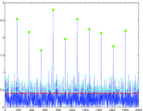
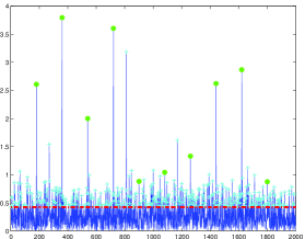
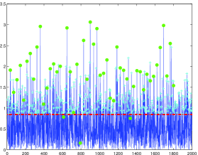
Exp1	Exp2	Exp3

Figure 1: Empirical second moment between $Y$ and $X_{1},\ldots,X_{p}$ for $p=2000$, $n=400$, the predictors $X^{\prime}$s are gaussian. Exp1: The predictors are independent, $S=10$. Exp2: The predictors are dependent, $s=10$. Exp3: The predictors are independent, $S=50$. The horizontal line is the auto-driven level $\hat{t}$.

The two successive thresholding steps of the algorithm are first detailed using the three different examples presented above. Figure 1 illustrates the first step of LOLA for the selection of the leaders for one experiment chosen among all $K=100$ experiments. All the scalar products $|\widetilde{X_{\ell}}^{t}Y|$ for $\ell=1,\ldots p=2000$ are represented in the picture; the estimated level $\hat{t}$ computed with procedure $A()$ is indicated with a horizontal line. The leaders are all the variables $\widetilde{X_{\ell}}$ with a scalar product $|\widetilde{X_{\ell}}^{t}Y|$ exceeding the threshold and are labeled with a small cross. let $\mathcal{L}$ denotes the set of leader indices. The indices belonging to $\mathcal{I}$ are circled to indicate the variables which should be rightly selected.

Observe that the reduction of the dimensionality is drastic: $N=144$ leaders are selected during the first step among the $p=2000$ initial predictors. When the sparsity is small and when the predictors are independent (see Exp1), the values of the scalar products of the predictors really involved in the model are close to the value of the coefficients (here $|\beta_{\ell}|\sim 2$). For Exp1, the first step is fine since any variable defined in $\mathcal{I}$ is chosen to be a leader. As the sparsity increases or when the predictors become dependent as it is the case for Exp2 or Exp3, the empirical scalar products between the predictors and the target may have more unstable behaviors leading to significant coefficients falling below the threshold $\hat{t}$ and as a consequence not selected as leaders during the first thresholding step. For Exp3, three variables $p_{0}\in\{612,790,1338\}$ which should be kept are eliminated at the first step and are definitively lost for selection.

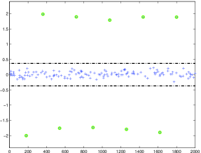
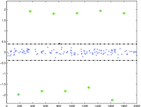
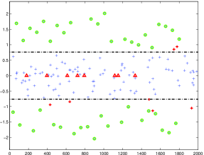
Exp1	Exp2	Exp3

Figure 2: Estimators of the linear coefficients $\beta_{\ell}$ for $\ell\in\mathcal{L}$ for $p=2000$, $n=400$, the predictors $X^{\prime}$s are gaussian. Exp1: The predictors are independent, $S=10$. Exp2: The predictors are dependent, $S=10$. Exp3: The predictors are independent, $S=50$. The horizontal lines are the auto-driven levels $\pm\,\hat{s}$.

Figure 2 illustrates the effect of the second thresholding of LOLA procedure for the same experiments for Figure 1.

The horizontal lines represent the levels $\pm\hat{s}$ where $\hat{s}$ is the output of procedure A( ). Figure 2 gives the estimated coefficients $\widehat{\beta_{\ell}}$ for $\ell\in\mathcal{L}$ computed with the OLS method restricted to the sub-set of predictors selected as leaders. The circle is the label for the coefficients $\widehat{\beta_{\ell}}$ with $\ell\in\mathcal{I}$ which are kept: this label allows to see the number TP of true positive detections. Triangular is the label for the coefficients $\widehat{\beta_{\ell}}$ with $\ell\in\mathcal{I}$ but which are below the level $\hat{s}$ (in absolute value): this label allows to see the number FN of false negative detections. Diamond is the label for the coefficients $\widehat{\beta_{\ell}}$ with $\ell\not\in\mathcal{I}$ which are kept by LOLA: this label allows to see the number FP of false positive detections. The results for Exp1 are excellent: both clusters of coefficients $\widehat{\beta_{\ell}}$ are well separated and A( ) algorithm performs in this situation very accurately; we obtain FN=FP=$0$ and we get exactly $\widehat{\mathcal{I}}=\mathcal{I}$. For Exp3, the separation between both clusters is not so straight and miss detections (triangular pattern) as false detections (cross not circled) are observed: FN$=8$ and FP$=7$.

The global performances obtained with $K$ experiments are presented in Table 1. For each column, the number of indices to be estimated is indicated into brackets. The first two columns focus on true detections and the last ones on false detections. Results for exp1 are perfect: LOLA algorithm selects always the right predictors and there is no error. When the sparsity $S$ increases, the results are less powerful: some predictors (FN$=13.9$) which should be selected by LOLA are finally not selected. Nevertheless, we observe that the number of false positive detections is again small (FP$=1.2$).

3.3 Conclusion and Comments

In order to be concise in this presentation, the above illustrations focused only on gaussian random variables with $SNR=5$. It should be stressed that an extensive simulation study has been conducted in parallel in order to evaluate the performances of LOLA. Various distributions for the predictors and different SNR have been implemented and studied. As conclusions to this experimental design, it can be stressed that for a given number of observations and potential predictors, the selection is more accurate for a low sparsity level. The number of false negatives and false positives tend to be null as the number of observations increases for a fixed number of predictors and/or the sparsity level decreases for a fixed number of predictors. It should be noted that very similar results are obtained if the Gaussian predictors are replaced by uniform, Bernoulli random variables or mixture of the above distributions.

As can be seen in Corollary 1, LOL procedure is consistent under a condition on the coherence $\tau_{n}\leq O\left(\sqrt{\log{p}/n}\right)$. This condition is verified with overwhelming probability for instance when the entries of the matrix $X$ are independent and identically random variables with a sub-gaussian common distribution but the results obtained in Exp2 show that the procedure is still working quite well even if this hypothesis is not satisfied. This fits a common fact in high dimensional setting, which is that the theoretical results are often more pessimistic than the true performances of the procedures. Moreover, before running the procedure, it should be noticed that the computation of $\tau_{n}$ brings some benefit as an indication of potential misbehaviors.

4 LOLA properties in a toy ’instrumental’ setting

We begin by studying the practical quality of our algorithm with real data combined with simulated instrumental data by revisiting the Boston Housing data set available from the UCI machine learning data base repository: http://archive.ics.ucfi.edu/ml/. One of our goal is here to evaluate the ability of LOLA procedure to accurately select the right predictors even if the original variables are embedded in a huge space built with artificial variables. This analysis also help to point out which kind of variables are wrongly selected from the complementary artificial space and which one are not selected from the initial space.

The original Boston Housing data are defined by one continuous target variable $Y$ (the median value of owner-occupied homes in USD) and $p_{0}=13$ predictive variables observed for $n=506$ observations. For our purpose, these original data are embedded in a high dimensional space of size $p=2100+13$ by adding artificially $300$ independent random variables of $7$ different laws: normal, $\log$normal, bernoulli, uniform, exponential, Student and Cauchy in equal proportion. This set of distributions is chosen to mimic the different empirical laws of the $p_{0}=13$ original predictive variables. In order to numerically evaluate the performances of LOLA, the procedure is called $K=100$ different times. Each time, a new set of artificial ’instruments’ has been simulated. Also, to evaluate the instability of the algorithm, each time the procedure has been performed on a 0.75$n$ sub-sample of the initial $n$- sample, randomly chosen.

Since the initial data are observed (and not simulated), we do not know in advance which variables should be selected in the model. In order to evaluate the performances of LOLA algorithm, we considered two benchmark procedures: a) the classical multiple regression following by variable selection using a simple Student test, b) the stepwise regression method (significant level 95%). Obviously, the two benchmark procedures are performed in the regular space of data with $p_{0}=13$ variables and $K=100$ times again by randomly choosing and $0.75\,n$ observations among the original data set.

In the high dimensional model ($p=2113$), the empirical coherence is $\tau_{n}=0.98$ which is very high and indicates that the predictors are very dependent. We applied LOLA procedure to this huge set of data. The results show that the number of false detections of the artificial variables is extremely low: we only select $92$ adding variables over 2100 random variables for a total of $K=100$ experiments. It is interesting to observe that half of the selected variables are distributed according to the cauchy law and $10\%$ are distributed according to the $T(2)$ law. A complementary work shows that the impact of heavy tailed distributions for the predictors is similar to the impact of dependence between predictors.

Figure LABEL:fig:3 shows the frequencies of detection for the initial $p_{0}=13$ predictors using LOLA procedure, OLS with Student test and stepwise regression. The results obtained with LOLA and OLS with Student test are similar very similar. This comparison confirms that our procedure performs fairly well in the presence of a huge number of artificial ’instrumental variables’.

This preliminary investigation, as a first step, as well as the previous simulation study, justifies the use in the sequel of LOLA as a selection algorithm in the presence of an important set of instrumental variables and make stronger our conclusions of the following section.

5 International Economic Growth

We study in this section the problem of convergence hypothesis in economic expounded in the introduction. We use the Barro and Lee data available from http://www.nber.org/pub/barro.lee. We present different models to evaluate the casual effect of a initial level $X$ of gross domestic product on the growth rate (of gross domestic product) using parametric models and economic variables as well as non-parametric models. Our aim is to empirically prove that the convergence hypothesis is valid and to compare our results with the results presented in Belloni and Chernozhukov (2010).

The Barro and Lee data are extracted as in Belloni and Chernozhukov (2010) and missing data are removed for each studied case. Notice that we restrict the number of countries ($n$) in the study since we want to take into consideration a large number of variables ($p$). It is important to keep this in mind for a further interpretation of the results.

5.1 The data

The national growth rate in gross domestic product (GDP) per capita is our dependent variable $Y$ and is studied for different periods of time. The predictor $X$ is an initial amount of the gross domestic product (GDP) per capita. More precisely, the variables are defined by $Y=\log\left({\mbox{GPD}_{t_{2}}/\mbox{GPD}_{t_{1}}}\right)$ and $X=\log(\mbox{GPD}_{t_{0}})$ for the following periods of time:

	Period $[t_{1},t_{2}]$	Initial Date $t_{0}$	$n$	$p$
Exp1	1965-75	1960	63	208
Exp2	1965-75	1965	63	208
Exp3	1975-85	1970	52	375
Exp4	1975-85	1975	52	375

The Barro and Lee data contain different economical indicators from 1960 to 1985. Six categories of variables are considered: Education (1), Population/Fertility (2), Governement Expendidures (3), PPP deflators (4), Political variables (5), Trade Policy and others (6).

In view to measure the accuracy of LOLA, as well as to increase the stability of the algorithm and also to see the impact of the sample of countries on the selection and estimation, we run the procedure $K=1000$ times using each time on a portion of $0.85n$ data randomly chosen from the initial data set. All the given results (the estimator $\hat{\alpha}_{2}$, the bounds of the confidence interval computed under the gaussian hypothesis, the $R^{2}$ and the p-value associated to the global Fisher test) are then averaged for the $K=1000$ experiments. The empirical standard deviation normalized by $\sqrt{K}$ is given into brackets. The indicator $N_{0}$ is the frequency of the even ”zero belongs to the confidence interval”. Ideally, $N_{0}=0$. The confidence intervals are computed for a coverage of $90\%$ which leads to test the null hypothesis $H_{0}:\;\alpha_{2}=0$ against $H_{1}:\;\alpha_{2}<0$ at the level $5\%$.

5.2 LOLA in a parametric setting

First, it should be noticed thanks to the results obtained by the standard OLS given in Table 2 that the linear model $Y=\alpha_{1}+\alpha_{2}X+u$ is irrelevant. For all periods of time, the $R^{2}$ is almost zero and the p-value leads to reject the significance of the model. Since $N_{0}=1$, the hypothesis $H_{0}:\;\alpha_{2}=0$ is always accepted at level $5\%$.

We now use LOLA procedure to select the subset of explanatory variables $Z_{\mbox{selected}}$ containing the maximum of information in order to explain $X$ or $Y$. Taking inspiration into the vast literature about instrumental variables in econometrics (see among many others Angrist, Imbens and Rubin (1996), Blundell and Powell (2003), Florens (2003), Darolles, Fan, Florens, Renault (2010) and Florens, Heckman, Meghir, Vytlacil (2003) in a nonparametric or semi-parametric framework), we select the instruments using the two following models

$$\mbox{Model 1:}\quad X=Z\beta+\mbox{error}\quad\mbox{ and }\quad\mbox{Model 2:}\quad Y=\alpha_{1}+\alpha_{2}X+Z\beta+\mbox{error}.$$

Depending on the situation, each of them has its own justification and interest: Model 1 is used in the first step of the Instrumental Variable method while Model 2 relies the endogeneity of $X$ in the initial model $Y=\alpha_{1}+\alpha_{2}X+u$ with the possibility that covariates $Z$ are missing. The selected instruments $Z_{\mbox{selected}}$ (obtained either via Model 1 or Model 2) are then used as control variables and we consider the following model

$$Y=\alpha_{1}+\alpha_{2}X+Z_{\mbox{selected}}\beta+\mbox{error},$$ (8)

where $\alpha_{1},\;\alpha_{2}$ and $\beta$ are estimated (OLS). For Model 1 (above) and Model 2 (below), we obtain the following results given in Table 3.

The selection via Model 2 seems to be more appropriate than the selection via Model 1: the p-value associated to the Fisher test is very small which leads to accept the significance of Model (Equation 8). We now focus on the results obtained with the selection using Model 2. Observe that the results concerning Exp1 and Exp2 (respectively Exp3 and Exp4) are very similar: the date $t_{0}$ of the initial amount of the GDP leads to similar results. The estimation of the coefficient $\alpha_{2}$ is negative and the confidence interval never contains zero (remember that the results are averaged on $K=1000$ experiments). Results are better for Exp1 (and Exp2) than for Exp3 (and Exp4): $N_{0}$ is equals $2\%$ for the first period of study instead of $30\%$ for the second period of study. Analyzing the empirical densities of the estimator $\hat{\alpha}_{2}$ given in Figure 4, we notice that for both periods of time, the support is almost included in $R^{-}$: for the period $1965-1975$ and $t_{0}=1960$, all of the runs provide negative estimated values while for the period $1975-1985$ and $t_{0}=1970$, 99.8% of the runs do.

Notice that the number of selected instruments is quite reasonable ($\hat{S}\sim 6$ or $8$) so we can also comment our results on a qualitative point of view. Incidentally, it is very interesting to identify the determinants of growth. To partially answer this question, Figure 5 shows the frequencies of selected variables using Model 2 when the growth rates under consideration are for both periods 1965-75 and 1975-85. The six vertical areas define the 6 broad categories of variables as given in the beginning of this part. It is interesting to notice that the sets of selected variables are quite different for both periods of time. For 1965-75, the most selected variables are indicators of the demography of the countries like ”Life expectancy at age 0” (1960, 1970, 1965-69, 1970-74) and ”Total Fertility rate” (1965-69) while for period 1975-85, they are ”Total gross enrollment ratio for secondary education” (1975), ”Male gross enrollment ratio for secondary education” (1965), ”Growth rate of population” (1965-69), ”Ratio of real government ”consumption” expenditure net of spending on defense and on education to real GDP” (1965-69) and ”Black market premium” (1975-79, 1980-84). This, of course can be partially due to the instability of the method, it may also have economical interpretations.

5.3 Comparison with results by Belloni and Chernozhukov

In Belloni and Chernozhukov (2010), a lasso procedure is used for the first period 1965-75. The method depends on a tuning parameter $\lambda$: the smaller is $\lambda$, the more instrument variables are selected and larger (in absolute value) is the estimator of $\alpha_{2}$. In the following table, we recall the results by Belloni and Chernozhukov (2010) when $\lambda$ is varying and our results when all the data are used ($K=1$) since no stability bootstrapping has been performed in Belloni and Chernozhukov (2010). Observe that the LOLA procedure leads to larger estimators of $\alpha_{2}$ (in absolute value) and confidence intervals which are better separated from zero. We verify that zero never belongs to the intervals of confidence obtained by LOLA procedure even if the level $\alpha$ becomes larger than $90\%$.

For 1965-75, the selected variables are ”Percentage of ”no schooling in the male population” (1970) and ”Percentage of ”primary school attained” in the total population and in the female population” (1970). These variables related to the education policy are also selected by Belloni and Chernozhukov (2010). It is striking that LOLA selects variables which are the same as in Belloni and Chernozhukov (2010). Recall that LOLA works in high dimension (here $p\sim 200$ or $300$) while the lasso procedure is used in the standard case where $p<n$ ($p\sim 40$). For the second period 1975-1985, LOLA retains

• ”Percentage of primary school complete in the female population” (1960, 1965)

• ”Population Proportion over 65” (1960)

• ”Growth rate of population” (average on 1980-84)

• ”Black market premium” (average on 1975-79, average on 1980-84)

as in Belloni and Chernozhukov (2010) and in addition

• ”Total gross enrollment ratio for secondary education” (1975, 1980)

• ”Total fertility rate” (1970, average on 1980-84)

• ”Life expectancy at age 0” (1975).

5.4 LOLA in a non-parametric setting

If we are only interested by the sign of the coefficient $\alpha_{2}$, it could be interesting to build a set of tailored instrumental variables which have no economical meaning but which provides a very good model

$$Y=\alpha_{2}X+\alpha_{1}+Z\beta+\mbox{ error}$$

in the sense that the number $\hat{S}$ of variables $Z$ is small and that the null hypothesis $H_{0}:\alpha_{2}=0$ is rejected. Using our own instruments has also another advantage: the study can be conducted with almost all the countries ($n\sim 110$) while half were removed in the previous part because pieces of information were missing for some variables: by instance China, Singapore were not considered for the first period of time and many countries from Africa were missing in the study for the second period.

As a consequence, let us consider the vector $X$ as a signal, and indeed replace $X$ by $X_{(.)}$ where $X_{(.)}$ is the vector such that $X_{(1)}\leq\ldots\leq X_{(n)}$ such a way that the curve of the initial amount of the GDP becomes smoother. Taking inspiration from the learning theory (see Kerkyacharian, Mougeot, Picard and Tribouley (2009) ), we build a set of functions called dictionary ${\mathcal{D}}$ containing the functions cosinus, sinus, box and Schauder:

$${\mathcal{D}}=\left\{\varphi_{\lambda}\right\}_{\lambda\in\Lambda}=\left\{\varphi^{1}_{\lambda_{1}},\varphi^{2}_{\lambda_{2}},\varphi^{3}_{\lambda_{3},}\varphi^{4}_{j,k}\quad\mbox{ for }1\leq\lambda_{1},\lambda_{2},\lambda_{3}\leq n,0\leq j\leq\log_{2}(n),1\leq k\leq 2^{j}-1\right\}$$

for

$$\varphi^{1}_{\lambda}(x) = \cos(2\pi\lambda\,x)\quad\mbox{ and }\quad\varphi^{2}_{\lambda}(x)=\sin(2\pi\lambda\,x)$$

$$\varphi^{3}_{\lambda}(x) = 1_{[a_{\lambda},b_{\lambda}]}(x)\mbox{ where }a_{\lambda},b_{\lambda}\backsim{\mathcal{U}}_{[0,n]}$$

$$\varphi^{4}_{j,k}(x) = 2^{j/2}\varphi^{3}(2^{j}x-k)\quad\mbox{ where }\quad\varphi^{4}(x)=\left(x1_{[0,0.5]}(x)\right)-\left(x1_{[0.5,1]}(x)-1\right).$$

For each function of the dictionary, the curve $Z_{\lambda}=\;^{t}\left(\varphi_{\lambda}\left(1/n\right),\ldots,\varphi_{\lambda}\left(i/n\right),\ldots,\varphi_{\lambda}\left(n/n\right)\right)$ is considered as an instrumental variable and the matrix $Z=\left(Z_{\lambda}\right)_{\lambda\in\Lambda}$ contains $p=\#{\mathcal{D}}$ predictors. Here, we get $n=110$ and $p=300$. The obtained results are excellent

Observe that the number of selected instruments is smaller than in the parametric setting as well as the fit is better if we are only concerned by the explanation of $Y$ by $X$. The confidence interval for $\alpha_{2}$ almost never contain zero: see the very small values of $N_{0}$. Again, we observe that the initial $t_{0}$ has no influence on the estimation of $\alpha_{2}$ and that the estimator is slightly smaller for the second period of time. In order to compare the non parametrical methodology with the parametrical methodology, we give again the empirical densities of the estimator $\hat{\alpha}_{2}$: here the results are excellent since their supports are strictly contained in $R^{-}$.

Finally, if we end this section with a rapid comparison with Belloni and Chernozhukov (2010), using all the available data in one run, we always accept the hypothesis $\alpha_{2}<0$. Notice that the number of selected instruments is again relatively small and is comparable to the number founded in Belloni, Chernozhukov (2010) for $\lambda=0.4$. Again, our estimators are further away from zero than the lasso estimators.

6 Proof of Theorem 1

Theorem 1 is an obvious consequence of Proposition 1.

The main ingredients for proving Proposition 1, are Lemma 1 and Lemma 2. These lemmas are proved in Mougeot, Picard and Tribouley (2010): see the terms $IBS$ and $OBB+OBS$ for Lemma 1 and the term $IBS$ for Lemma 2 and put $\alpha_{\ell}=\sigma_{\ell}\,\beta_{\ell}$ and $\widehat{\alpha_{\ell}}=\sigma_{\ell}\,\widehat{\beta_{\ell}}$.

Lemma 1.

Recall that ${\mathcal{J}}$ is the set of the indices of the leaders defined in (1). Assume that the sparsity conditions (2) are satisfied by the sequence $(\beta_{\ell}),\ell=1,\ldots,p$. For any $\lambda\geq C\left(S\tau_{n}^{2}+S\log{p}/n\right)$ where $C$ is a computable constant depending on $\eta^{2}$ and $\sum_{\ell=1}^{p}|\sigma_{\ell}\beta_{\ell}|$, we get

$$P\left(\sum_{\ell\in\Omega_{\iota}}\;|\sigma_{\ell}\beta_{\ell}|^{2}\;\;>\;\lambda\right)\leq 2\exp\left(-c\,\frac{n\lambda}{\eta^{2}}\right)\quad\mbox{ for }\iota=1,2,$$

with

$$\Omega_{1}=\{\ell=1,\ldots,\;p,\;|\sigma_{\ell}\beta_{\ell}|\geq 2s_{n},\,|\sigma_{\ell}\widehat{\beta_{\ell}}|\leq s_{n}\}$$

and

$$\Omega_{2}=\{\ell=1,\ldots,\;p,\;\ell\not\in{\mathcal{J}},\,|\sigma_{\ell}\beta_{\ell}|\geq 2t_{n}\}$$

and where $c$ is an universal constant.

Lemma 2.

Recall that ${\mathcal{J}}$ is the set of the indices of the leaders defined in (1). Assume that the sparsity conditions (2) are satisfied by the sequence $(\beta_{\ell}),\ell=1,\ldots,p$ and choose threshold levels $t_{n},s_{n}$ such that $t_{n}>s_{n}\vee C\left(\tau_{n}+\sqrt{\log{p}/n}\right)$. Then, for any $\lambda\geq C\left(S/n\right)$ where $C$ is a constant depending on $\sigma^{2}$ and $M$, we get

$$P\left(\sum_{\ell\in\Omega_{3}}\;|\sigma_{\ell}\widehat{\beta_{\ell}}-\sigma_{\ell}\beta_{\ell}|^{2}\;\;>\;\lambda\right)\leq\exp\left(-c\,\frac{n\lambda}{\sigma^{2}}\right)$$

with

$$\Omega_{3}=\{\ell\in{\mathcal{J}},\;|\sigma_{\ell}\beta_{\ell}|\leq s_{n}/2,\,|\sigma_{\ell}\widehat{\beta_{\ell}}|\geq s_{n}\}$$

and where $c$ is an universal constant.

Now, we are ready to prove Proposition 1. First, we focus on $FN$. Using (4), and for $\mu_{n}>s_{n}/2$, we get

$$\#(\mathcal{I})=\#\left(\{\ell,\;|\sigma_{\ell}\beta_{\ell}|\geq\mu_{n}\}\right)\leq S\leq\lfloor\tau_{n}^{-1}\rfloor$$

and we conclude applying Lemma 1 with $\mu_{n}\geq 2(s_{n}\vee t_{n})$. More precisely, for a given $k$, we get

$$P(FN>k) =P(\#(\mathcal{I}\cap(\widehat{\mathcal{I}})^{c})\;>\;k)$$

$$=P(\#\{\ell,\;|\sigma_{\ell}\beta_{\ell}|\not=0,|\sigma_{\ell}\widehat{\beta_{\ell}}|\,{\mathbb{I}}\{|\sigma_{\ell}\widehat{\beta_{\ell}}|\geq s_{n}\}=0\}\;>\;k)$$

$$\leq P(\sum_{\ell=1}^{p}|\sigma_{\ell}\beta_{\ell}|^{2}\;{\mathbb{I}}\{\,|\sigma_{\ell}\beta_{\ell}|\geq\mu_{n}\}\;{\mathbb{I}}\{\,|\sigma_{\ell}\widehat{\beta_{\ell}}|\,{\mathbb{I}}\{|\sigma_{\ell}\widehat{\beta_{\ell}}|\geq s_{n}\}=0\}\;>\;k\mu_{n}^{2})$$

$$\leq P(\sum_{\ell\in\Omega_{1}}\;|\sigma_{\ell}\beta_{\ell}|^{2}\;>\;k\mu_{n}^{2}/2)+P(\sum_{\ell\in\Omega_{2}}\;|\sigma_{\ell}\beta_{\ell}|^{2}\;>\;k\mu_{n}^{2}/2)$$

$$\leq 2\exp\left(-c\;\frac{nk\mu_{n}^{2}}{2\sigma^{2}}\right)$$

as soon as

$$k\;\mu_{n}^{2}/(2\sigma^{2})\geq c^{\prime}\,\left(M^{2}\;\tau_{n}^{2}\vee\frac{1}{n}\vee\frac{|\log{\tau_{n}}|}{n}\right)\,S.$$

Similarly, applying Lemma 2 with $t_{n}>s_{n}\vee C\left(\tau_{n}+\sqrt{\log{p}/n}\right)$, we get

$$P(FP>k) =P(\#(\mathcal{I}^{c}\cap\widehat{\mathcal{I}})\;>\;k)$$

$$=P(\#\{\ell,\;|\sigma_{\ell}\beta_{\ell}|\geq\mu_{n},|\sigma_{\ell}\widehat{\beta_{\ell}}|\,{\mathbb{I}}\{|\sigma_{\ell}\widehat{\beta_{\ell}}|\geq s_{n}\}\not=0\}\;>\;k)$$

$$\leq P\left(\sum_{\ell\in\Omega_{3}}\;|\sigma_{\ell}\widehat{\beta_{\ell}}-\sigma_{\ell}\beta_{\ell}|^{2}\;\;>\;ks_{n}^{2}\right)\;\leq\exp\left(-c\;\frac{nks_{n}^{2}}{\sigma^{2}}\right)$$

a soon as

$$k\;\frac{s_{n}^{2}}{\sigma^{2}}\geq c\,\frac{S}{n}.$$

References

Angrist, J., G. Imbens, and D. R. Rubin.

(1996). Identification of Causal Effects Using Instrumental Variables. Journal of the American Statistical Association, 91, pp 444–455.

Barro, R. and Lee, J.-W.

(1994). Data set for a panel of 139 countries.

Barron A. R., Cohen A., Dahmen, W. and DeVore, R. A.

(2008). Approximation and learning by greedy algorithms. The Annals of Statistics, 36, pp 64–94.

Belloni, A. and Chernozhukov, V

(1999). $L_{1}$-penalized quantile regression in high-dimensonal sparse models. ArXiv e-prints

Bickel, P. J., Ritov, Y. and Tsbybakov, A.

(2008). Simultaneous analysis of Lasso and Dantzig selector. ArXiv e-prints

Blundell, R. and Powel, J.

(2003). Endogeneity in Nonparametric and Semiparametric Regression Models, Cambridge Univ. Press., Advances in Economics and Econometrics: Theory and Applications, 2, pp 312–350.

Bunea, F., Tsbybakov, A. and Wegkamp, M.

(2007). Sparsity oracle inequalities for the Lasso, Electronic Journal of Statistics, 1, pp 169–194.

Candes, E. and Tao, T..

(2007). The Dantzig selector: statistical estimation when $p$ is much larger than $n$ The Annals of Statistics, 35, pp 2313–2351.

Darolles, S. and Fan, Y. and Florens, J.-P. and Renault, R.

(2010). Nonparametric Instrumental Regression, IDEI Working Paper, 228 .

Fan, J. and Lv, J.

(2008). A Selective Overview of Variable Selection in High Dimensional Feature Space. Journal of the Royal Statistic Society B, 70, pp 849–911.

Fan, J. and Lv, J.

(2010). Sure independence screening for ultrahigh dimensional feature space Statistica Sinica, 20, pp 101–148.

Florens, J.P..

(2003). Inverse problems and structural econometrics: The example of instrumental variables. Cambridge Univ. Press., In Advances in Economics and Econometrics: Theory and Applications, 2, pp 284-311.

Florens, J.-P. and Heckman, J. and Meghir, C. and Vytlacil, E.

(2003). Instrumental Variables, Local Instrumental Variables and Control Functions, IDEI Working Paper , 249.

Haury, A.-C., Jacob, L. and Vert, J.-P.

(2010). Increasing stability and interpretability of gene expression signatures, ArXiv e-prints .

Kerkyacharian, G., Mougeot, M., Picard, D. & Tribouley, K.

(2009). Learning Out of Leaders, Multiscale, Nonlinear and Adaptive Approximation. Lecture Notes in Comput. Sci. Springer.

Mougeot, M., Picard, D. & Tribouley, K.

(2010). Learning Out of Leaders. ArXiv e-prints

Needell, D. and Tropp, J. A.

(2009). CoSaMP: iterative signal recovery from incomplete and inaccurate samples Applied and Computational Harmonic Analysis, 26, pp 301–321.

Sala-I-Martin, X.

(1997). I Just Ran Two Million Regressions. The American Economic Review, 87, pp 178–183.

Tibshirani, R.

(1996). Regression Shrinkage and Selection via the Lasso. Journal of the Royal Statistical Society B, , 58, pp 267-288.

Tropp, Joel A. and Gilbert, Anna C.

(2007). Signal recovery from random measurements via orthogonal matching pursuit. Institute of Electrical and Electronics Engineers. Transactions on Information Theory, 53, pp 4655–4666.

	TN	TP	FN	FP
Exp1	1990.0 (1990)	10.0 (10)	0.0 (0)	0.0 (0)
Exp2	1989.9 (1990)	9.2 (10)	0.8 (0)	0.7 (0)
Exp3	1948.8 (1950)	36.1 (50)	13.9 (0)	1.2 (0)

Table 1: Simulations performances for $K=100$ replications. The true target value is given into brackets.

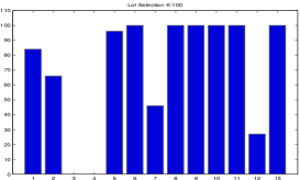
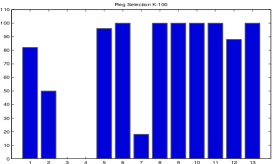
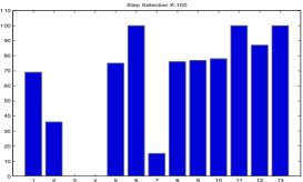
LOLA ($p=1213$)	OLS Student Selection($p=13$)	STEP ($p=13$)

Figure 3: Variables selection performances for Boston data, $K=100$

	$\widehat{\alpha_{2}}$	Confidence Interval	$N_{0}$	$R^{2}$	p-value for $F$ test
Exp1	0.012	[-0.038 , 0.062 ]	1.000	0.005	0.673
Exp2	0.017	[-0.031 , 0.065 ]	1.000	0.008	0.577
Exp3	0.051	[-0.002 , 0.104 ]	1.000	0.045	0.139
Exp4	0.058	[ 0.006 , 0.111 ]	1.000	0.060	0.085

TABLE 2: Estimation of the model $Y=\alpha_{1}+\alpha_{2}X+u$ for the different periods of time. All the standard deviation values normalized by $\sqrt{1000}$ are smaller than $10^{-3}$.

	$\hat{S}$	$\widehat{\alpha_{2}}$	CI	$N_{0}$	p-value for $F$ test
Exp1	10.8 (0.1)	-0.245 (0.002)	[-0.358 (0.002), -0.132 (0.002)]	0.011 (0.003)	0.013 (0.001)
Exp2	10.9 (0.1)	-0.225 (0.002)	[-0.342 (0.002), -0.109 (0.002)]	0.039 (0.006)	0.025 (0.002)
Exp3	14.2 (0.1)	-0.227 (0.004)	[-0.429 (0.004), -0.025 (0.004)]	0.452 (0.015)	0.155 (0.005)
Exp4	14.6 (0.1)	-0.175 (0.004)	[-0.434 (0.005), 0.083 (0.004)]	0.742 (0.014)	0.255 (0.006)
Exp1	6.3 (0.1)	-0.246 (0.002)	[-0.342 (0.002), -0.150 (0.001)]	0.016 (0.004)	0.007 (0.041)
Exp2	6.3 (0.1)	-0.232 (0.002)	[-0.331 (0.002), -0.132 (0.001)]	0.025 (0.005)	0.011 (0.042)
Exp3	8.4 (0.1)	-0.166 (0.003)	[-0.266 (0.003), -0.066 (0.002)]	0.230 (0.013)	0.004 (0.017)
Exp4	8.4 (0.1)	-0.149 (0.003)	[-0.262 (0.003), -0.036 (0.002)]	0.311 (0.014)	0.009 (0.034)

TABLE 3: Estimation of $\alpha_{2}$ for determinants $Z$ selected via Model 1 (above) and Model 2 (below).

FIGURE 4. Exp1: 1965-75, $t_{0}=1960$, empirical density of $\hat{\alpha}_{2}$	Exp3: 1975-85, $t_{0}=1970$, empirical density of $\hat{\alpha}_{2}$

FIGURE 5. Selected variables for different periods 1965-1975, $t_{0}=$ 1960 (bottom) and 1975-1985, $t_{0}=$1970 (below). Area 1: Education, Area 2: Population/Fertility, Area 3: Governement Expendidures, Area 4: PPP deflators, Area 5: Political variables, Area 6: Trade Policy and others.

	M	$\lambda$	$\hat{S}$	$\widehat{\alpha_{2}}$	CI
Exp1	BC	1.183	2	-0.016	[-0.025, -0.004]
Exp1	BC	0.788	4	-0.041	[-0.054, -0.029]
Exp1	BC	0.591	3	-0.044	[-0.065, -0.034]
Exp1	BC	0.473	11	-0.051	[-0.065, -0.032]
Exp1	M2		3	-0.136	[-0.212 , -0.060 ]
Exp2	M2		3	-0.116	[-0.191 , -0.040 ]
Exp3	M2		11	-0.351	[-0.442 , -0.261 ]
Exp4	M2		11	-0.332	[-0.443 , -0.221 ]

TABLE 4. Estimation of $\alpha_{2}$ for selection obtained via lasso procedure and LOLA for Model2.

	$\hat{S}$	$\widehat{\alpha_{2}}$	CI	$N_{0}$
Exp1	7.964	-0.116	[-0.146 , -0.085 ]	0.001
Exp2	7.896	-0.115	[-0.144 , -0.085 ]	0.000
Exp3	7.958	-0.130	[-0.165 , -0.096 ]	0.002
Exp4	7.769	-0.139	[-0.172 , -0.106 ]	0.000
Exp1	8.772	-0.085	[-0.099 , -0.072 ]	0.002
Exp2	8.736	-0.083	[-0.097 , -0.070 ]	0.005
Exp3	8.766	-0.096	[-0.111 , -0.080 ]	0.004
Exp4	8.773	-0.094	[-0.109 , -0.079 ]	0.002

TABLE 5. Estimation of $\alpha_{2}$ for various periods of time and for predictors $Z$ selected via Model1 (above) and Model2 (below). All the standard deviation values normalized by $\sqrt{1000}$ are smaller than $10^{-3}$.

FIGURE 6. Exp1: 1965-75, $t_{0}=1960$, empirical density of $\hat{\alpha}_{2}$	Exp3: 1975-85, $t_{0}=1970$, empirical density of $\hat{\alpha}_{2}$

	$\hat{S}$	$\widehat{\alpha_{2}}$	CI		$\hat{S}$	$\widehat{\alpha_{2}}$	CI
Exp1	8	-0.120	[-0.148 , -0.092 ]		8	-0.086	[-0.098 , -0.073 ]
Exp2	8	-0.116	[-0.144 , -0.089 ]		8	-0.083	[-0.095 , -0.071 ]
Exp3	8	-0.133	[-0.165 , -0.100 ]		9	-0.100	[-0.114 , -0.085 ]
Exp4	7	-0.140	[-0.172 , -0.108 ]		9	-0.093	[-0.107 , -0.079 ]

TABLE 6. Estimation of $\alpha_{2}$ for both periods of time and for determinants $Z$ selected via Model1 (left) and Model2 (right).