The dynamic thermal expansivity of liquids near the glass transition.

Abstract

Based on previous works on polymers by Bauer et al. [Phys, Rev. E (2000)], this paper describes a capacitative method for measuring the dynamical expansion coefficient of a viscous liquid. Data are presented for the glass-forming liquid tetramethyl tetraphenyl trisiloxane (DC704) in the ultraviscous regime. Compared to the method of Bauer et al. the dynamical range has been extended by making time-domain experiments and by making very small and fast temperature steps. The modelling of the experiment presented in this paper includes the situation where the capacitor is not full because the liquid contracts when cooling from room temperature down to around the glass-transition temperature, which is relevant when measuring on a molecular liquid rather than polymer.

The glass transition occurs when the configurational degrees of freedom of a liquid are frozen in. Below the glass transition temperature, $T_{g}$, only isostructural contraction takes place as temperature is decreased further. The measured thermal expansion coefficient, $\alpha$ (and heat capacity, $c_{p}$) are therefore lower in the glass than in the equilibrium liquid. This change of the thermal expansion coefficient (and the heat capacity), is probably the most classical signature of the glass transition, and a figure illustrating this change (see Fig. 1) is almost inevitably the starting point of introductory talks or texts on the glass transition (eg. Ref. Angell et al., 2000; Dyre, 2006).

Figure 1: Illustration of the temperature dependence of volume and expansion coefficient of a liquid in the vicinity of the glass-transition. Upon cooling the expansivity decreases abruptly at the glass transition. This gives rise to a kink in the temperature dependence of the volume. These features are the original signatures of the glass transition.

The change in the heat capacity at the glass transition $\Delta c_{p}=c_{p,liq}-c_{p,glass}$ has been studied extensively and is widely believed to play a role for the dynamics of liquids close to the glass transition. The change in expansion coefficient $\Delta\alpha_{p}=\alpha_{p,liq}-\alpha_{p.glass}$ has received less attention, but is of similar importance. This is seen, for instance, in the literature related to the Prigogine-Defay ratio, a dimensionless number characterizing the glass transition Davies and Jones (1953); Prigogine and Defay (1954); Goldstein (1963); Moynihan and Gupta (1978); Ellegaard et al. (2007).

The glass is an out-of-equilibrium state and therefore the values of the thermodynamic derivatives are not rigorously well defined. They depend on cooling rate and also on the time spent in the glassy state. Contrary to this the linear response of the metastable equilibrium liquid state is well defined and history independent Ellegaard et al. (2007). The linear expansion coefficient of a viscous liquid close to its glass transition is dynamic, that is time (or frequency) dependent with short times giving a low (glass-like) value, $\alpha_{p,fast}$, while long times give a higher liquid value, $\alpha_{p,slow}$. The difference between these two levels $\Delta\alpha_{p,lin}=\alpha_{p,slow}-\alpha_{p,fast}$ thus gives well-defined information on the configurational part of the expansion coefficient. Likewise $\Delta c_{p,lin}=c_{p,slow}-c_{p,fast}$ is well defined.

The relaxation between the fast and the slow response takes place on a certain time scale which is temperature dependent. Considered in this way the measurement of the expansion coefficient can be viewed as a type of spectroscopy, which gives both a relaxation time and a spectral shape analogous to other methods like dielectric spectroscopy or mechanical spectroscopy. The study of the temperature dependence of relaxation times and of the spectral shape of different response functions is vital for understanding the viscous slowing down. There is a general belief that the liquid has a relaxation time, which is fairly well defined independent of probe, but also suggestions that different processes may decouple from each other at low temperatures Angell (1991).

There are good scientific reasons to study the dynamic linear expansion coefficient, but almost no data of this type are to be found in literature. The time-dependent expansion coefficient can be found by studying the change in volume as a function of time after a temperature step. Such volume relaxation experiments are very classic in glass science and still important Kovacs (1958); Greiner and Schwarzl (1989); Kolla and Simon (2005); Svoboda et al. (2006). However, volume relaxation experiments are traditionally performed as non-linear aging experiments, i.e., with large amplitudes in the temperature jump. This type of experiment gives information on the relaxation of the configurational degrees of freedom, but the expansion coefficient and its characteristic time scale cannot be determined, because the results depend on the amplitude and sign of the temperature jump. For sufficiently small temperature steps this is not the case, defining the linear response regime.

The only linear dynamic data we are aware of were reported about a decade ago by Bauer et al. Bauer et al. (2000a, b) followed by a paper by Fukao and Miyamoto Fukao and Miyamoto (2001). These papers reported frequency-domain measurements on thin polymer films, performed with temperature scans at a couple of fixed frequencies, covering 1.5 decade of the dynamics. The measurements were pioneering, but 1.5 decade is not very much for studying relaxation in viscous liquids, because the relaxation is extremely temperature dependent and quite “stretched”, which means that even at one fixed temperature the relaxation covers several decades.

The technique developed by Bauer et al. is based on a principle where the sample is placed in a parallel plate capacitor such that it is the sample that maintains the spacing between the plates. Thus a change in sample volume in response to temperature change leads to a change of the capacitance. This principle is also used in the present work. The advantage of this technique is that capacitance can be measured with high accuracy and it is this accuracy which makes linear experiments possible.

The use of sample-filled capacitors for measuring an expansion coefficient is not unique and it has been done by others before and after Bauer et al. (see eg. Ref. Meingast et al., 1996; Fukao and Miyamoto, 1999; Serghei et al., 2006; Oh and Green, 2009) in capacitative scanning dilatometry, i.e. working in a temperature ramping mode. Capacitative scanning dilatometry has to our knowledge never been used on simple liquids. It is particularly useful for studying thin polymer films because the signal gets better with a thin sample. The technique has been used for determining the glass-transition temperature for example as a function of film thickness Fukao and Miyamoto (1999); Serghei et al. (2006) or as a function of cooling rate Meingast et al. (1996). The main focus of these papers is on the temperature dependence of the expansion coefficient, while little attention is given to the absolute values. There have been no studies of the dynamics since the pioneering work of Bauer and no attempts to extend the dynamical range.

To the best of our knowledge there are no measurements of the dynamic linear expansion coefficient of molecular liquids. The reported data from scanning dilatometry and non-linear volume relaxation are also mainly for polymers, while data on molecular liquids is relatively scarce. This may be due to the higher technological importance of polymers. It is probably also related to the fact that working with molecular liquids requires other experimental conditions, meaning that techniques developed for polymers are not always directly applicable to liquids.

This paper gives a description of an experimental method developed for measuring the dynamical expansion coefficient of a viscous. As mentioned, the principle is based on the capacitive technique by Bauer et al. Bauer et al. (2000a, b). The method is modified in three respects compared to the work of Bauer et al.: 1) The modelling takes into account the situation where the capacitor is not full, which is relevant when measuring on a molecular liquid rather than on a polymer. 2) The experiment is performed in the time domain using a very fast temperature regulation, which gives a dynamical range of more than four decades. 3) The sensitivity is enhanced by using a capacitance bridge with a very high resolution. This makes it possible to measure the response following very small temperature steps, ensuring that the response is close to perfectly linear. As an application of the technique the paper presents data on the glass-forming liquid tetramethyl tetraphenyl trisiloxane (DC704) in the ultraviscous regime.

I Response functions with consistent dimensions

In a linear response experiment, the response of a system to an external perturbation is studied. If the perturbation is small the output is assumed to be linearly dependent on the input. The formalism to describe this is well known. However, different formulations can be used, and the version used in this work when converting the measured time-domain response to the frequency-domain response function is maybe not the most common one. The formalism used here has the advantage that the time-domain response function and the frequency-domain response function have the same dimension and there is no differentiation involved when transforming between the two. This section gives a summary of the response function formalism used including a comparison to the standard formalism.

The fundamental assumption is that the output depends linearly on the input. The most general statement is that the change in input $dI(t^{\prime})$ at time $t^{\prime}$ leads to a contribution in output $dO(t)$ at time $t$:

$$dO(t)=R(t-t^{\prime})dI(t^{\prime}).$$ (1)

It is here assumed that the change in output only depends on the time difference $(t-t^{\prime})$. Causality implies that

$$R(t)=0\textrm{ for }t<0.$$ (2)

Integrating on both sides of Eq. (1):

$$O(t)=\int^{t}_{-\infty}R(t-t^{\prime})dI(t^{\prime}),$$

and substituting $t^{\prime\prime}=t-t^{\prime}$ and writing $\dot{I}(t)=\dfrac{dI(t)}{dt}$

$$O(t) = -\int_{\infty}^{0}R(t^{\prime\prime})\dot{I}(t-t^{\prime\prime})dt^{\prime\prime}.$$

Changing $t^{\prime\prime}$ to $t^{\prime}$:

$$O(t)=\int^{\infty}_{0}R(t^{\prime})\dot{I}(t-t^{\prime})dt^{\prime}.$$ (3)

If the input is a Heaviside function:

$$I(t)=I_{0}H(t)=I_{0}\left\{\begin{array}[]{rl}0&\textrm{for }t\leq 0\\ 1&\textrm{for }t>0\end{array}\right.$$

then

$$O(t)=I_{0}\int^{\infty}_{0}R(t^{\prime})\delta(t-t^{\prime})dt^{\prime}=I_{0}R(t),$$ (5)

and it is seen that $R(t)$ is the output from a Heaviside step input.

Linear response can also be studied in the frequency domain. In the case of a harmonic oscillating input $I(t)=I_{0}e^{i(\omega t+\phi_{I})}$, the output $O(t)=O_{0}e^{i(\omega t+\phi_{O})}$ will be a periodic signal with the same frequency $\omega$, but there will be a phase shift of the output relative to the input. From Eq. (3) the output is

$$O(t) = \int^{\infty}_{0}R(t^{\prime})i\omega I_{0}e^{i\phi_{I}}e^{i\omega(t-t^{\prime})}dt^{\prime}$$

$$= I_{0}e^{i\omega t}e^{i\phi_{I}}i\omega\int^{\infty}_{0}R(t^{\prime})e^{-i\omega t^{\prime}}dt^{\prime}$$

$$= I(t)R(\omega),$$

where $R(\omega)$ is the frequency domain response function, which is given by the Laplace transform of $R(t)$ times $i\omega$:

$$R(\omega)=i\omega\int^{\infty}_{0}R(t^{\prime})e^{-i\omega t^{\prime}}dt^{\prime}.$$

The linear response relation is often expressed in an alternative formulation where the linearity assumption is expressed by

$$O(t) = \int^{t}_{-\infty}\mu(t-t^{\prime})I(t^{\prime})dt^{\prime},$$

where $\mu$ is sometimes called the memory function, but it is also sometimes called the response function. The use of the word response function for $\mu(t)$ is somewhat inconvenient because it has a different dimension compared to the frequency-domain response function $R(\omega)$. Substituting again ($t^{\prime\prime}=t-t^{\prime}$) and changing $t^{\prime\prime}$ to $t^{\prime}$

$$O(t) = \int_{0}^{\infty}\mu(t^{\prime})I(t-t^{\prime})dt^{\prime}.$$

Applying a Heaviside input again

$$O(t) = \int^{\infty}_{0}\mu(t^{\prime})I_{o}H(t-t^{\prime})dt^{\prime}$$ (6)

$$= I_{0}\int^{t}_{0}\mu(t^{\prime})dt^{\prime}.$$

From Eq. (5) and (6) we have

$$R(t)=\int_{0}^{t}\mu(t^{\prime})dt^{\prime},$$

and therefore

$$\dfrac{dR(t)}{dt}=\mu(t).$$ (7)

In the memory function formalism the frequency domain response is again found by inserting a harmonic oscillating input. In this case the result becomes

$$R(\omega)=\int^{\infty}_{0}\mu(t^{\prime})e^{-i\omega t^{\prime}}dt^{\prime}=\int^{\infty}_{0}\dfrac{dR(t)}{dt}e^{-i\omega t^{\prime}}dt^{\prime},$$

where the last equality comes from inserting Eq. (7). This expression is formally equivalent to Eq. (23) which can be shown by integration by parts and by invoking $R(t=0)=0$. However, when converting data in practice Eq. (23) has the advantages that differentiation of the time domain data is avoided. It is always good to avoid differentiation of numerical data because it introduces increased noise. Moreover, if we introduce an “instantaneous” response in terms of $R(t\rightarrow 0)\neq 0$ corresponding to very short times where we can not measures the time dependence of the response, then this information would be lost by differentiation.

II Principle, design and procedure

The method requires that there is a simple relation between sample density and dielectric constant. The dielectric constant in general has two contributions: atomic polarization and rotational polarization Böttcher (1973). The atomic polarization is due to the displacement of the electron cloud upon application of a field. This contribution is governed by the microscopic polarizability of the molecule, $x$ (usually called $\alpha$, but $\alpha$ is reserved for the expansivity in this paper). The atomic polarizability can be assumed to be temperature and density independent in the relevant range. This means that the desired simple relation between density and dielectric constant can be obtained when the atomic polarization is the only contribution.

The rotational polarization is due to rotation of the permanent dipoles in the sample. This contribution is relevant when the liquid has a permanent dipole moment and mainly at frequencies lower than or comparable to the inverse relaxation time of the liquid. The rotational contribution gives the dielectric signal monitored in standard dielectric spectroscopy. The rotational polarization is temperature-, density- and frequency-dependent, and it is therefore non-trivial to relate the density to the dielectric constant when rotational polarization is present. Therefore, in capacitative dilatometry it is a contribution one would like to avoid. It is sometimes assumed that the high frequency plateau value of the dielectric constant measured in dielectric spectroscopy contains only atomic polarization and that it corresponds to the square of refraction index $n^{2}$. However, there is also fast (“glass-like”) contribution to the rotational part of the polarization. The fast rotational contribution will dominate over the geometric effects even at high frequencies if the sample has a high dipole moment. This was demonstrated in Ref. Niss et al., 2005. To minimize the rotational contribution two things are done: 1) Only liquids with very small dipole moment are studied - i.e. liquids in which the atomic polarization is dominant at all frequencies and temperatures. 2) These liquids are only studied at frequencies much higher than the inverse relaxation time. In the data reported in this paper the measuring frequency is 10 kHz and the relaxation time is 100 seconds or more.

The cell is a capacitor made of circular copper plates of 1 cm diameter and 1 mm thickness, with a 50 $\mu$m spacing. The separation is kept by four 0.5 mm x 0.5 mm and 50 $\mu$m thick Kapton spacers. The spacing between the capacitor plates is filled with the sample liquid. The thin spacing results in a reasonably large dielectric signal (empty capacitance is 14 pF) despite the small size. The thin spacing moreover makes it possible to heat or cool the sample fast, even though the heat diffusion in the sample liquid is slow compared to the heat diffusion in the copper plates.

The cell is integrated with a microregulator, which is a tiny temperature regulator based on an NTC-thermistor (placed in the lower cupper plate of the capacitor-cell), a Peltier-element acting as a local source of heating and cooling, and an analog PID-control. The integrated cell and microregulator are placed in our main kryostat. With this setup the temperature of the sample can be changed by steps of up to 2 K within less than 10 s and the temperature can be kept stable is within a few micro Kelvin over days and weeks. The cell is shown in Fig. (2) and the whole system of the main kryostat and the microregulator is described in detail in Ref. Igarashi et al., 2008a.

The principle of the experiment is to make an “instantaneous” step in temperature and subsequently measure the capacitance at a fixed frequency as a function of time. From the capacitance we calculate the time-dependent expansion coefficient. In order for the temperature step to be “instantaneous” compared to the time scale of the relaxation we need the relaxation time to be 100 s or longer. This means that the measurements are performed at or below the conventional glass-transition temperature. Nevertheless, it is important to emphasize that, the liquid is in equilibrium when the experiment is performed because we wait at least five relaxation times whenever stepping to a new temperature before making a measurement. The measurements themselves also must be carried out over five relaxation times in order to obtain the relaxation curve all the way to equilibrium. All together, it takes days and sometimes even weeks to take a spectrum at a given temperature. This means that the experiment would be impossible without the stable temperature control ensured by the microregulator.

The relaxation time of viscous liquids close to the glass transition is extremely temperature dependent. We therefore need to make small temperature steps in order for the measured response to be linear. This means that the change in volume and thereby the measured capacitance is very small, the relative changes in capacitance $\textrm{d}C/C$ are of order 10^-4. We use an AH2700A Andeen Hagerling ultra-precision capacitance bridge, which measures capacitance with an accuracy of 5 ppm and true resolution of 0.5 attoFarad in the frequency range 50 Hz-20 kHz. The capacitance is measured every second at 10 kHz.

Figure 2: Schematic drawing of the dielectric measuring cell with the microregulator. The liquid is deposited in the 50 $\mu$m gap between the discs of the dielectric cell. The Peltier element heats or cools the dielectric cell, depending on the direction of the electrical current powering the element. The current is controlled by an analog temperature-control system that receives temperature feedback information from an NTC thermistor embedded in one disc of the dielectric cell (reproduced from Ref. Hecksher et al., 2010).

.

The sample used is liquid at room temperature and the capacitor is filled by letting the liquid suck in using the capillary effect. Complete filling is checked by measuring the capacitance before and after filling, comparing to the measured dielectric constant measured at the same temperature with a larger capacitor (which is easy to fill).

III Geometry and boundary conditions

In order to model the relation between the measured change in capacitance and the expansion coefficient some assumptions must be made regarding the behavior of the liquid during the experiment. In this section we describe these assumption and the arguments on which they are based.

The capacitor is filled completely at room temperature with a low viscosity molecular liquid. The measuring temperatures (close to and below the conventional glass-transition temperature) are typically around 100 degrees below room temperature for these types of liquids. The cooling makes the liquid contract in the radial direction because the distance between the plates is maintained by the spacers (which have a much smaller expansion coefficient). This has the consequence that the capacitor is not completely filled at the temperatures where the measurements take place. This gives rise to a difference compared to the measurements done on polymers in earlier work Bauer et al. (2000a, b), a difference which is taken into account when calculating the relation between the expansion coefficient and the change in capacitance in the following section.

The liquid contracts/expands radially as long as it has low viscosity, but the situation changes when the liquid gets ultraviscous. At high viscosities the liquid gets clamped between the plates due to the small distance between them. This has the consequence that the liquid can no longer contract/expand upon cooling/heating by flowing radially, but will contract/expand vertically and pull/push the plates changing the distance between them. This effect is the basis for the measurement, because the vertical expansion makes the capacitance change, and we calculate the expansion from the change in capacitance.

The distance between the plates is kept by the Kapton spacers at high temperatures (and long times) when the sample liquid flows. However, at times where the sample cannot flow, it is the sample, not the Kapton spacers which determines the distance. This is true because Kapton has a stiffness Davidson et al. (1992) of the same order of magnitude as the sample (in the GPa-range), but only takes up approximately 1% of the area between the plates.

The temperature change gives rise to an internal pressure, which is released by pressure diffusion via viscous flow. The characteristic time $\tau_{flow}$ of the radial flow between two plates of fixed distance $l$ can be estimated by the following argument. A temperature step of $\Delta T$ initiates an internal pressure $\Delta p=K_{T}\alpha_{p}\Delta T$ in the liquid. This creates a radial flow that eventually discharges the surplus volume $\Delta V=\Delta T\alpha_{p}\pi R^{2}l$. Although the volume flows in the radial direction we may as a crude estimation take the volume velocity, $\dot{V}$, of planar Pouiseuille flowLautrup (2005) $\dot{V}=\frac{\Delta p}{12\eta L}Wl^{3}$, where $L$ (the dimension in the direction of the flow) can be taken as $R$, and $W$ (the dimension perpendicular to the flow) can be taken as $2\pi R$. The characteristic discharge flowtime then becomes $\tau_{f}low=\frac{\Delta V}{\dot{V}}=6\frac{\eta}{K_{T}}(\frac{R}{l})^{2}$. The bulk modulus and the shear modulus are of the same order of magnitude. It follows that the Maxwell relaxation time is roughly given by $\tau_{M}\simeq\eta/K_{T}$ and that $\tau_{flow}\propto(R/l)^{2}\tau_{M}$. In the experiment we have $l$=50 $\mu$m and $R=5$ mm from which it follows that the radial flow time is ten thousand times longer than the Maxwell time. The alpha relaxation time is roughly given by the Maxwell time, the flow time will be more than ten days when the alpha relaxation time is one hundred seconds. This means that the liquid can be considered as radially clamped in the region we study (where all relaxation times are longer than 100 seconds). The transition between the radial flow and the clamped situation can be seen in dielectric constant when it is measured as a function of temperature, and the observed behavior is consistent with the above estimate.

The expansion coefficient we study with the boundary conditions described above is not the conventional isobaric expansion coefficient, $\alpha_{p}=\left.\frac{1}{V}\frac{\partial V}{\partial T}\right|_{p}$, because the liquid is clamped in two directions and only free to move in one direction. We call this expansion coefficient the longitudinal expansion coefficient, in analogy to the longitudinal modulus, (another name for it could be the iso-area expansion coefficient). It is expressed by $\alpha_{l}=\left.\frac{1}{V}\frac{\partial V}{\partial T}\right|_{A}=\left.\frac{1}{l}\frac{\partial l}{\partial T}\right|_{A}$, where $A$ is the constant area and $l$ is the dimension which is free to respond to the temperature change. The longitudinal expansion coefficient is related to the isobaric expansion coefficient $\alpha_{p}$ via the following relation

$$\alpha_{l}(\omega)=\frac{1}{1+\frac{4G(\omega)}{3K_{T}(\omega)}}\alpha_{p}(\omega).$$

Where $G$ is the shear modulus and $K_{T}$ is the isothermal bulk modulus, which are both dynamic i.e. frequency or time dependent as are the thermal expansion coefficients.

From this expression we see that $\alpha_{l}$ is smaller than $\alpha_{p}$, except at low frequencies (long times, or high temperatures) where $G=0$ which implies $\alpha_{l}=\alpha_{p}$. This expression for the longitudinal expansion coefficient is given (but not derived) in another equivalent form in terms of the Possoin’s Ratio in Refs. Fukao and Miyamoto, 1999; Bauer et al., 2000a; Wallace et al., 1995 and can be derived from row 3 of Eq. (53) in Ref. Christensen et al., 2007. Also note that there is a total lack of standard notation. Bauer et al. use $\alpha_{p}$ to note the linear expansion coefficient, which is the quantity often used to express volume expansion of solids. That is their $\alpha_{p}$ is 1/3 of our $\alpha_{p}$. The linear expansion coefficient is called $\alpha_{L}$ by Wallace et al. Wallace et al. (1995), while Fukao et al. Fukao and Miyamoto (1999) call it $\alpha_{\infty}$. The quantity we call the longitudinal expansion coefficient $\alpha_{l}$ is denoted $\alpha_{CA}$ (CA for clamped area) by Bauer, $\alpha_{N}$ by Wallace and $\alpha_{n}$ by Fukao (n for normal).

IV Relating the measured change in capacitance to $\alpha_{l}$

IV.1 Deriving the relation

In the measurement we perform a small temperature step $\delta T$ and subsequently measure the capacitance $C_{m}$ as a function of time. From the measurements we find the time dependent quantity $\frac{1}{C_{m}}\frac{\Delta C_{m}}{\Delta T}(t)$. In the following section we show that this quantity is proportional to the expansion coefficient, $\alpha_{l}(t)$, with a proportionality constant that depends on $\epsilon_{\infty}$ and the degree of filling of the capacitor, $f$, but not on the geometrical capacitance or the distance between the plates.

The starting point is that the only contribution to the high-frequency dielectric constant, $\epsilon_{\infty}$, is the atomic polarizability (Sec. II). We moreover use the Lorentz field Böttcher (1973) from which it follows that dielectric constant is given by the Clausius-Mossotti relation:

$$\frac{\epsilon_{\infty}-1}{\epsilon_{\infty}+2}=\frac{n}{3\epsilon_{0}}x,$$

where $x$ is the polarizability of a single molecule, $n$ is the number density of molecules, and $\epsilon_{0}$ is the vacuum permeability.

Moreover, we assume that we have a parallel plate capacitor which is partially filled with a dielectric liquid. The degree of filling is denoted by $f$ and the measured capacitance is given by

$$C_{m}=f\epsilon_{\infty}\frac{A\epsilon_{0}}{l}+(1-f)\frac{A\epsilon_{0}}{l}=\left[f\epsilon_{\infty}+(1-f)\right]C_{g}$$ (8)

where $C_{g}=\frac{A\epsilon_{0}}{l}$ is the geometrical capacitance of the empty capacitor at the given temperature.

The derivative with respect to temperature is now given by

$$\frac{\mathrm{d}C_{m}}{\mathrm{d}T}=\left[f\epsilon_{\infty}+(1-f)\right]\frac{\mathrm{d}C_{g}}{\mathrm{d}T}+C_{g}f\frac{\mathrm{d}\epsilon_{\infty}}{\mathrm{d}T}.$$ (9)

Here it is assumed that the liquid does not contract radially at the temperatures (and on the time scale) we consider (see Sec. III), thus $\textrm{d}f/\textrm{d}T=0$. The next step is to calculate $\frac{\mathrm{d}C_{g}}{\mathrm{d}T}$ and $\frac{\mathrm{d}\epsilon_{\infty}}{\mathrm{d}T}$ under the assumption that the area is constant. This was done by Bauer Bauer et al. (2000a, b). For completeness we include a detailed derivation as an Appendix. The result is

$$\frac{\mathrm{d}\epsilon_{\infty}}{\mathrm{d}T}=-K(\epsilon_{\infty})\alpha_{l}$$ (10)

where $K(\epsilon_{\infty})$ is given by $K(\epsilon_{\infty})=(\epsilon_{\infty}-1)(\epsilon_{\infty}+2)/3$ and

$$\frac{\mathrm{d}C_{g}}{\mathrm{d}T}=-C_{g}\alpha_{l}\,.$$ (11)

Inserting Eq. (10) and (11) in Eq. (9) yields

$$\frac{\mathrm{d}C_{m}}{\mathrm{d}T}=\left[f\epsilon_{\infty}+(1-f)\right](-C_{g}\alpha_{l})-C_{g}fK(\epsilon_{\infty})\alpha_{l}$$

$$=-C_{g}\left[f\epsilon_{\infty}+(1-f)+fK(\epsilon_{\infty})\right]\alpha_{l}\,.$$

Inserting $C_{g}=C_{m}/\left[f\epsilon_{\infty}+(1-f)\right]$ and dividing by $C_{m}$ leads to

$$\frac{1}{C_{m}}\frac{\mathrm{d}C_{m}}{\mathrm{d}T}=-\frac{f\epsilon_{\infty}+(1-f)+fK(\epsilon_{\infty})}{f\epsilon_{\infty}+(1-f)}\alpha_{l}\,.$$ (12)

Isolating finally $\alpha_{l}$ gives

$$\alpha_{l}=-\frac{f\epsilon_{\infty}+(1-f)}{f\epsilon_{\infty}+(1-f)+fK(\epsilon_{\infty})}\frac{1}{C_{m}}\frac{\mathrm{d}C_{m}}{\mathrm{d}T}$$

$$\alpha_{l}=P(f,\epsilon_{\infty}))\frac{1}{C_{m}}\frac{\mathrm{d}C_{m}}{\mathrm{d}T},$$ (13)

where

$$P(f,\epsilon_{\infty})=-\frac{f\epsilon_{\infty}+(1-f)}{f\epsilon_{\infty}+(1-f)+fK(\epsilon_{\infty})}$$

IV.2 The absolute value of $\alpha_{l}$

The determination of $\alpha_{l}$ and also the uncertainties of the measured value depend on determining correctly the proportionality constant $P(f,\epsilon_{\infty})$. In order to do so we need to determine the relevant values of $f$ and $\epsilon_{\infty}$. To find $f$ we use the expansion coefficient and to find the dielectric constant $\epsilon_{\infty}$ we use the measured empty capacitance along with the measured full capacitance.

The high-temperature expansion coefficient is found Gundermann (2012) to be 0.7*$10^{-3}$ $K^{-1}$; at low temperatures we find There is a small step of iteration involved in the data treatment here, since we use the expansion coefficient we find to get a more precise value of it. that it is around 0.5*$10^{-3}$ $K^{-1}$ in the long time limit. We use 0.6*$10^{-3}$ $K^{-1}$ as an average value, and find from this that the degree of filling is $f=0.95$ if the liquid is assumed to contract radially down to 213 K where the relaxation time is 100 s. The choice of expansion coefficient in the range 0.5-0.7*$10^{-3}$ $K^{-1}$ and final temperatures in the range 210-215 K makes $f$ change with $\pm 1$%. The effect of changing $f$ within this range leads only to $\pm 0.5$% changes in $P(f,\epsilon_{\infty})$.

Isolating the dielectric constant from Eq. (8) gives:

$$\epsilon_{\infty}=\frac{C_{m}-C_{g}(1-f)}{fC_{g}}$$ (14)

From this it is seen that the uncertainty in $f$ also gives an uncertainty in $\epsilon_{\infty}$, and this actually has a greater impact on the uncertainty of $P$ than the direct effect of the uncertainty on $f$. Including this effect, the uncertainty in $P$ due to uncertain degree on filling is still only $\pm 1$%.

In order to determine $\epsilon_{\infty}$ from Eq. (14) we need to know the geometric capacitance, $C_{g}$. This is found from measurements on the empty capacitor at the measuring temperature. We estimate that the uncertainty is $\pm 2$% on $C_{g}$. This estimate is made by comparing measurements made on the capacitor after assembling it anew. The total uncertainty on $\epsilon_{\infty}$ is roughly $\pm 3$%, which leads to an uncertainty on $P$ of $\pm 2$%.

Altogether the uncertainty on $P(f,\epsilon_{\infty})$ and therefore on the absolute value of $\alpha_{l}$ is about $\pm 3$%. It should be emphasized that this uncertainty has no effect on the shape or the time scale of the measured relaxation. This is so as long as we stick to linear experiments. For larger temperature steps there will be (at least in principle) some second-order effects making $P(f,\epsilon_{\infty})$ change during the relaxation because of the change in $\epsilon_{\infty}$.

In the modelling of the connection between measured change in capacitance to $\alpha_{l}$ we have not considered the radial expansion of the electrode plates. Including this (in the simples possible way) gives rise to an extra additive term $\frac{1}{C_{m}}\frac{\epsilon_{0}}{l}\frac{\mathrm{d}A}{\mathrm{d}T}$ in Eq. (12). The size of this term will be given by the linear expansion coefficient of the electrodes. They are in this case made of copper, which at the relevant temperature has a linear expansion of approximately $15\times 10^{-6}$ K^-1. The total measured change in the capacitance is about 50-100 times bigger, thus the effect is small. However, the time dependence is different therefore it could be relevant to include this effect in the future. Alternatively we also consider shifting to an electrode material with an even smaller expansion coefficient in order to avoid the effect all together.

It should be kept in mind that we have used the Lorentz field. This is an important assumption and the use of an other local field, when connecting density with the dielectric constant will change the result. Using the macroscopic Maxwell field, will yield the same everywhere, except for $K(\epsilon_{\infty})$ in Eq. (10) which will be given by $K_{Max}(\epsilon_{\infty})=(\epsilon_{\infty}-1)$ instead of the $K_{Lor}(\epsilon_{\infty})=(\epsilon_{\infty}-1)(\epsilon_{\infty}+2)/3$. This leads to a 20 % increase in $P$ and the calculated numerical value of $\alpha_{l}$. Again we stress that using another local field will change the absolute values, but will not change the time scale or shape of the measured relaxation.

While none of the above-mentioned things affect the time scale or the spectral shape of the measured relaxation, the temperature dependence of $\epsilon_{\infty}$ could in principle affect the temperature dependence of the calculated $\alpha_{l}$. However, this effect is negligible over the 6 degree range studied in the work and $P$ will be considered constant.

To summarize, the problems discussed in this section can lead to an unknown temperature- and frequency-independent scaling of all the measured $\alpha_{l}$-values.

IV.3 The shape of the relaxation curve

In the following we describe the measuring protocol in detail and describe a correction made on the data. We moreover use this to give an estimate of the uncertainty on the shape of the relaxation curves reported.

A main issue is, of course, the first part of the measuring curve where the temperature gets in equilibrium. Fig. (3) shows details of a single temperature step. It is clearly seen how the target temperature is achieved within less than 10 s, corresponding to a characteristic time of 2 s.

Fig. (4) a) shows a typical set of temperature steps: a series of up and down jumps are made at the same temperature, with variable amplitude.

Figure 3: Zoom on the temperature monitored in the NTC-bead in the lower capacitor plate during the first 40 seconds of at temperature step.

Fig. (4) b) shows the raw measured capacitance corresponding to the temperature steps in Fig. (4) a). Two things are worth noticing. First we see the expected rise in capacitance when temperature is decreased. Secondly, we see a long time drift of the equilibrium level.

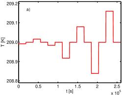
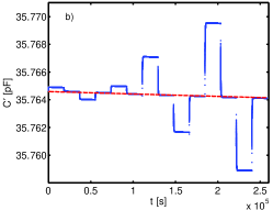
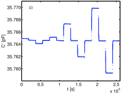
Figure 4: a) Example of temperature protocol at one temperature. A series of up and down jumps are made at the same reference temperature with different amplitude. The temperatures shown are those measured with the NTC-bead in the lower capacitor plate. Notice that the smallest jumps are 0.01 K. b) The measured capacitance (blue points). Notice that the relative changes in capacitance ($\textrm{d}C/C$) for the small jumps is less than 10^-4 and can still be measured precisely. There is a long time drift in the measured capacitance, the dashed line illustrates this background drift and this slope is subtracted of the data before further treatment.
c) The measured capacitance after subtraction of the drift.

At low temperatures where the liquid cannot contract radially it contracts vertically. Comparing measurements on the empty capacitor with liquid filled measurements we estimate that the expansion coeficient of the liquid is roughly 10 times larger than that of the Kapton spacers. This means that the liquid compresses the Kapton. However, on very long times it will be the Kapton which dominates (becuase the liquid flows) and the Kapton will therefore slowly relax and press the electrodes apart. We believe that this effect is what leads to the long time drift seen in Fig. (4) b).

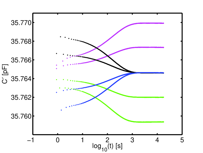
Figure 5: The corrected measured capacitance shown on a logarithmic time scale with the temperature change as starting time. The temperature steps with the same final temperature (shown in black and blue) all have the same final value of the capacitance. The data shown here correspond to the last 8-steps in Fig. (4)

The drift is subtracted before treating the data, as illustrated in Fig. (4) c) and Fig. (5).

We make both up jumps and down jumps in temperature and the subtraction of the drift has an opposite effect on the two. We can therefore check that the subtraction is made correctly by comparing up jumps and down jumps. This is illustrated in Fig. (6). The superposition of data obtained in up and down jumps also demonstrates that the experiment is linear and gives a general estimate of how precise the determination of the curve shape is.

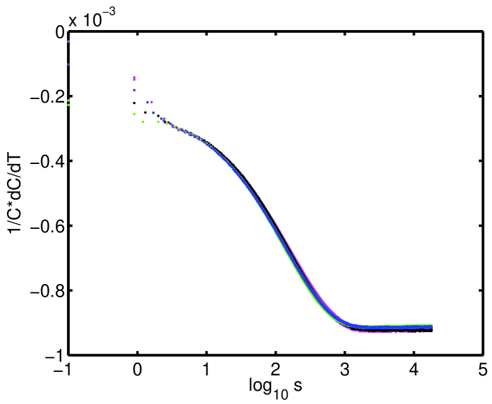
Figure 6: The relative change in C divided by the size of the temperature step. The data shown are the same data as in Fig. (5) and the colors used for each curve is the same. All the curves superpose, which demonstrates that the experiment is linear. Moreover it demonstrates that the subtraction of the background drift is successful.

The comparison of up and down jumps moreover serves to guarantee that the steps are linear. The relaxation time is strongly temperature dependent when the liquid is close to the glass transition, and the steps therefore have to be very small in order to maintain linear behavior. Smaller steps can be made as well, and the shape of the relaxation is maintained, but the curve starts to get noisy because the signal is very small. When we make larger temperature steps, we begin to get typical non-linear aging behavior. That is, the relaxation is slower for down jumps than for up jumps when the final temperature is the same. The setup is actually well suited for nonlinear experiments also; because of the extremely high resolution of the measured quantity we get very well-defined curves and can clearly see the nonlinear behavior already at steps of 1 degree. We plan to use the setup for these types of studies, as well, but focus in this paper on the linear results.

V Data

Fig. (7) shows the expansion coefficient as a function of time at four different temperatures. The data are shown for steps made with $\approx$0.1 K, except the data at 211 K which are taken with a temperature step of $\approx$0.01 K. This is why there is more noise on this dataset.

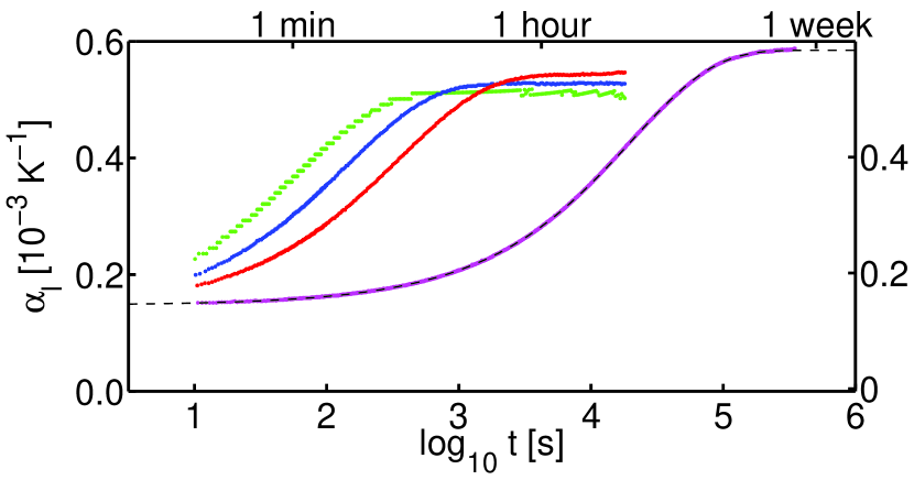
Figure 7: The measured time dependent expansion coefficient of Tetramethyltetraphenyltrisiloxane at T= 205 K, 209 K, 210 K and 211 K. At the lowest temperature we also show a fit to the modified stretched exponential Sağlanmak et al. (2010).

Fig. (8) shows all the data from Fig. (7) normalized and superimposed. This illustrates that the measured relaxation obeys time-temperature-superposition (TTS) within the studied (relatively narrow) temperature range. The fit shown in figure 7 is a fit to the superimposed curve obtain from the datasets at T=205 K and T=211 K.

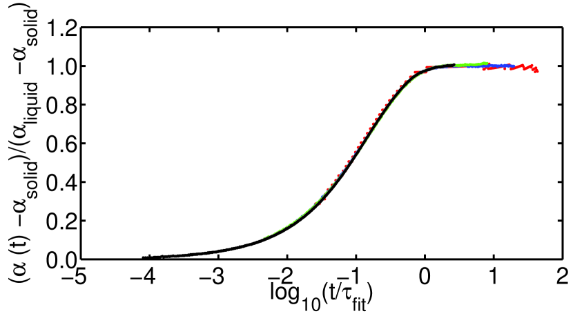
Figure 8: The data from Fig. (7) normalized and plotted versus time scaled with the relaxation time (as defined from the fit to the modified stretched exponential). The figure demonstrates that the data obey time temperature superposition (TTS).

The function used to fit the date is a modified stretched exponential Sağlanmak et al. (2010) given by:

$$\alpha(t)=\alpha_{\infty}+\Delta\alpha\left(1-\exp\left[-k\left(\frac{t}{\tau}\right)^{\beta}-\frac{t}{\tau}\right]\right).$$ (15)

In the fit to data we get $\beta=0.6$ and $k=2.6$. The quality of the fit is so good that we have used it as an interpolation of the data and used it to calculate the frequency-domain response, which is given by the transformation in Eq. (23). The transformation is made by making a discrete Fourier transform (using matlabs FFT-procedure) on the fit of the normalized curve evaluated in a number of points. The transformed normalized curve is shown in Fig. (9). Here we also show an Exponential relaxation which has been transformed using the same algorithm along with the analytical Laplace transform. Moreover, the high frequency power law, which corresponds to the exponent of the fit, is also shown.

Figure 9: Illustration of the Laplacetransform. Cyan Diamonds: Laplace Transform of the normalized data (found by brute force nummerical integration of the measured points). Blue: Laplacetransform of the normalized fit (see text for details). Red: Exponential relaxation which has been transformed using the same algorithm as the used for the fit. Black dashed : analytical Laplace transform of Exponential relaxation. Blue dashed-dotted line: power law, which corresponds to the exponent of the fit.

In Fig. (10) we show the Laplace transformed fit rescaled with amplitudes and time scales in order to show the temperature dependence of the frequency dependent thermal expansion coefficient.

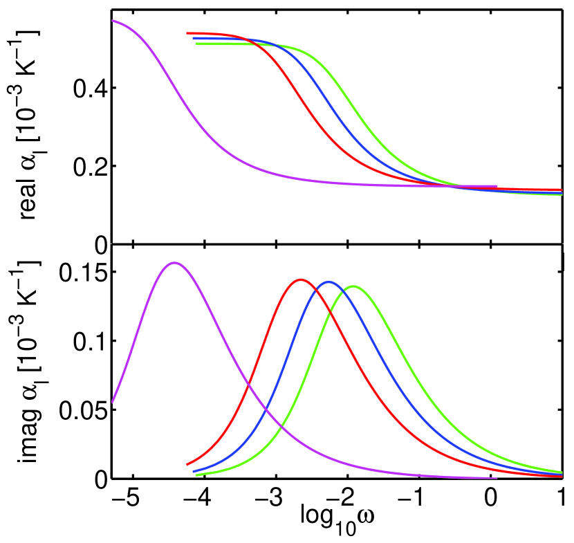
Figure 10: Laplace transformed fits (see the text for details). The curves are shown a in the dynamical range that roughly corresponds to the measurement.

VI Summary and outlook

We have presented a technique for measuring the dynamical expansion coefficient $\alpha(t)$ for a glass-forming liquid in the ultraviscous range. The experiment is performed on a setup which follows the capacitative principle suggested by Bauer et al. Bauer et al. (2000a). The dynamical range has been extended from 1.5 decade to more than four decades by making time-domain experiments, and by making very small and fast temperature steps. The modelling of the experiment has moreover been developed. Data is presented on the molecular glass-former tetramethyl tetraphenyl trisiloxane (DC704). This data set is to the best of our knowledge the first data on the dynamical expansion coefficient of a molecular liquid.

The technique presented in this paper is based on a principle where the sample is placed in a parallel plate capacitor such that the sample maintains the spacing between the plates. Thus a change in sample volume in response to a temperature change leads to a change of the capacitance. The advantage of this technique is that capacitances can be measured with very high precision, and the small density changes associated with linear experiments can therefore be determined reliably. One limitation of the technique is that it only works on timescales larger than 10 s, this could possibly be overcome by smaller samples and thereby faster temperature control. A more intrinsic limitation is that the technique only works for samples with very small dipole moment. For samples with large dipole moment we therefore need a complementary technique.

The measurements of the thermal expansivity is part of a general ambition in the “Glass and Time” group to measure different response function of viscous liquids. A unique feature of our techniques is that the all fit into the same type of cryostat Igarashi et al. (2008a), ensuring that the absolute temperature of the liquid is the same for all measurements. The thermal expansion measurements described in this paper are thus performed in the same cryostat as our shear mechanical spectroscopy Christensen and Olsen (1995), bulk mechanical spectroscopy Christensen and Olsen (1994), specific heat spectroscopy Jakobsen et al. (2010) and dielectric spectroscopy Igarashi et al. (2008b). The properties of liquids close to the glass transition are extremely temperature dependent, and small differences in the temperature calibration can lead to rather large differences in the results. Measuring different response functions at the exact same conditions therefore makes it possible to analyze new aspects of the viscous slowing down and the glass transition. In recent papers we used this to compare time scales of all the different response functions Jakobsen et al. (2011), to relate linear response to density scaling and to determine the linear Prigogine Defay ratio Gundermann et al. (2011).

VII Acknowledgments

The center for viscous liquid dynamics “Glass and Time” is sponsored by the Danish National Research Foundation (DNRF). Ib Høst Pedersen, Torben Rasmussen, Ebbe Larsen and Preben Larsen are thanked for their contribution to development of the temperature control and the measuring cell. Niels Boye Olsen is thanked for sharing his experience and ideas. Tina Hecksher and Bo Jakobsen are thanked for fruitful discussions.

Appendix I

The relation between the temperature derivative of the dielectric constant and of the geometrical capacitance with the longitudinal expansion coefficient was derived by Bauer Bauer et al. (2000a, b). For completeness we include a detailed derivation in this Appendix.

The longitudinal expansion coefficient is defined by

$$\alpha_{l}=\frac{1}{l}\left(\frac{\partial l}{\partial T}\right)_{A}$$ (16)

We start with the temperature derivative of $\epsilon_{\infty}$, which in this situation is given by:

$$\left(\frac{\partial\epsilon_{\infty}}{\partial T}\right)=\left(\frac{\partial\epsilon_{\infty}}{\partial l}\right)_{A}\left(\frac{\partial l}{\partial T}\right)_{A}$$ (17)

so we need and expression for the first term, $\left(\frac{\partial\epsilon_{\infty}}{\partial l}\right)_{A}$. The Clausius-Mossotti relation gives

$$\frac{xN}{3\epsilon_{0}Al}=\frac{(\epsilon_{\infty}-1)}{(\epsilon_{\infty}+2)}$$ (18)

where $N$ is the total number of molecules, $A$ is the area and $l$ is the thickness such that $N/(Al)$ is the number density of molecules and $x$ the microscopic polarizability of the molecule.

We rewrite this to get

$$\epsilon_{\infty}=\frac{xN}{3\epsilon_{0}Al}\left(\epsilon_{\infty}+2\right)+1$$

and take the derivative with respect to $l$ at constant $A$

$$\left(\frac{\partial\epsilon_{\infty}}{\partial l}\right)_{A}=\frac{xN}{3\epsilon_{0}Al}\left(\frac{\partial\epsilon_{\infty}}{\partial l}\right)_{A}-(\epsilon_{\infty}+2)\frac{xN}{3\epsilon_{0}Al^{2}}$$

which by reinserting Eq. (18) gives

$$\left(\frac{\partial\epsilon_{\infty}}{\partial l}\right)_{A}=\frac{(\epsilon_{\infty}-1)}{(\epsilon_{\infty}+2)}\left(\frac{\partial\epsilon_{\infty}}{\partial l}\right)_{A}-(\epsilon_{\infty}+2)\frac{1}{l}\frac{(\epsilon_{\infty}-1)}{(\epsilon_{\infty}+2)}.$$

We now isolate $\left(\frac{\partial\epsilon_{\infty}}{\partial l}\right)_{A}$ in this expression and get

$$\left(\frac{\partial\epsilon_{\infty}}{\partial l}\right)_{A}=-\frac{1}{l}\frac{(\epsilon_{\infty}-1)(\epsilon_{\infty}+2)}{3}$$

inserting this in Eq. (17)

$$\left(\frac{\partial\epsilon_{\infty}}{\partial T}\right)_{T}=-\frac{(\epsilon_{\infty}-1)(\epsilon_{\infty}+2)}{3}\frac{1}{l}\left(\frac{\partial l}{\partial T}\right)_{A}$$

which when comparing to the definition of the longitudinal expansion coefficient in Eq. (16) can be rewritten as

$$\left(\frac{\partial\epsilon_{\infty}}{\partial T}\right)_{T}=-\frac{(\epsilon_{\infty}-1)(\epsilon_{\infty}+2)}{3}\alpha_{l}=-K(\epsilon_{\infty})\alpha_{l}$$

where the last equality comes from defining $K(\epsilon_{\infty})=\frac{(\epsilon_{\infty}-1)(\epsilon_{\infty}+2)}{3}$

Now we move on to the temperature derivative of the geometrical capacitance, $C_{g}$, which in this situation is given by:

$$\left(\frac{\partial C_{g}}{\partial T}\right)=\left(\frac{\partial C_{g}}{\partial l}\right)_{A}\left(\frac{\partial l}{\partial T}\right)_{A}$$ (19)

The geometrical capacitance itself is given by

$$C_{g}=\frac{A\epsilon_{0}}{l}$$

giving

$$\left(\frac{\partial C_{g}}{\partial l}\right)_{A}=-\frac{A\epsilon_{0}}{l^{2}}=-\frac{1}{l}C_{g}$$

which when inserted in Eq. (19) and combined with the definition of the longitudinal expansion coefficient gives

$$\left(\frac{\partial C_{g}}{\partial T}\right)_{A}=-C_{g}\alpha_{l}.$$ (20)

VIII Appendix II : FD-theorem and the expansion coefficient

This appendix gives the formal definition of the dynamic expansion coefficient, including how it relates to fluctuations and how the frequency-domain response is related to the measured time-domain response. This is and extension of the presentation in Ref. Bauer et al., 2000a. However, Ref. Bauer et al., 2000a contains a typo as well some definitions which are not precise regarding the absolute levels of the response functions. The precise definitions are important for our use of the data in Ref. Gundermann et al., 2011.

The measured response to an external field, whether in the time domain or in the frequency domain, is directly related to the equilibrium thermal fluctuations of the system. This is expressed formally through the fluctuation dissipation theorem (FDT), which expressed in the time domain isDoi and Edwards (1986); Nielsen and Dyre (1996):

$$\dfrac{dR(t)}{dt}=-\dfrac{1}{k_{B}T}\dfrac{d}{dt}\langle\Delta A(t)\Delta B(0)\rangle.$$ (21)

Here $R(t)$ is the response function (see Sec. (I) for a definition) and sharp brackets refers to ensemble averages. $A$ is the measured physical quantity (that is the output $O(t)$ in Sec. (I)) and $B$ is conjugated to the applied input/field, which is called $I(t)$ in Sec. (I). The function $\langle\Delta A(t)\Delta B(0)\rangle$ is the correlation function, which in the simple case where $A=B$ reduces to the auto correlation function.

Integrating on both sides of Eq. (21) and inserting $R(t=0)=0$ gives the time-domain response function :

$$\int_{0}^{t}\dfrac{dR(t^{\prime})}{dt}dt^{\prime} = -\int^{t}_{0}\dfrac{1}{k_{B}T}\dfrac{d}{dt^{\prime}}\langle\Delta A(t^{\prime})\Delta B(0)\rangle dt^{\prime}$$

$$R(t) = \dfrac{1}{k_{B}T}(\langle\Delta A(0)\Delta B(0)\rangle-\langle\Delta A(t)\Delta B(0)\rangle).$$ (22)

from which it is seen that $R(t=0)=0$ as it should be. The frequency-domain response function, is given by the Laplace transform of $R(t)$ times $i\omega$:

$$R(\omega)=i\omega\int^{\infty}_{0}R(t^{\prime})e^{-i\omega t^{\prime}}dt^{\prime}.$$ (23)

Combining this with Eq. (VIII) gives the FDT in the frequency domain:

$$R(\omega) = -\dfrac{i\omega}{k_{B}T}\int^{\infty}_{0}\langle\Delta A(t)\Delta B(0)\rangle-\langle\Delta A(0)\Delta B(0)\rangle e^{-i\omega t}dt$$ (24)

$$= \dfrac{1}{k_{B}T}\langle\Delta A(0)\Delta B(0)\rangle-\dfrac{i\omega}{k_{B}T}\int^{\infty}_{0}\langle\Delta A(t)\Delta B(0)\rangle e^{-i\omega t}dt.$$

Considering now a linear experiment where a small temperature step $\delta T$ is applied to a system at constant pressure at $t=0$. Its volume response is subsequently measured as a function of time:

$$\delta V(t)=R(t-t^{\prime})\delta T(t^{\prime}),$$ (25)

then the response function $R(t)$ is given by $R(t)=\frac{\delta V(t)}{\delta T}$ (see Sec. I for more details on the linear response formalism). The time-dependent isobaric expansion coefficient is defined by

$$\alpha_{p}(t) = \dfrac{1}{V}\frac{\delta V(t)}{\delta T}$$ (26)

$$= \dfrac{R(t)}{V}$$

In terms of the FDT (Eq. (VIII)), the relevant fluctuations for $\alpha_{p}(t)$ are volume and entropy, and the expansion coefficient can therefore be expressed in the following way:

$$\alpha_{p}(t) = \dfrac{1}{Vk_{b}T}\left(\langle\Delta V(0)\Delta S(0)\rangle-\langle\Delta V(t)\Delta S(0)\rangle\right).$$ (27)

The frequency-domain response function $\alpha_{p}(\omega)$ is then (from Eq. (24))

$$\alpha_{P}(\omega)=\dfrac{1}{Vk_{B}T}\langle\Delta V(0)\Delta S(0)\rangle-\dfrac{i\omega}{Vk_{B}T}\int^{\infty}_{0}\langle\Delta V(t)\Delta S(0)\rangle e^{-i\omega t}dt.$$ (28)

References

- Angell et al. (2000) C. A. Angell, K. L. Ngai, G. B. McKenna, P. F. McMillan, and S. W. Martin, J. Appl. Phys. 88, 3113 (2000).
- Dyre (2006) J. C. Dyre, Rev. Mod. Phys. 78, 953 (2006).
- Davies and Jones (1953) R. O. Davies and G. O. Jones, Adv. Phys. 2, 370 (1953).
- Prigogine and Defay (1954) I. Prigogine and R. Defay, Chemical Thermodynamics (Longmans, London, 1954).
- Goldstein (1963) M. Goldstein, J. Chem. Phys. 39, 3369 (1963).
- Moynihan and Gupta (1978) C. T. Moynihan and P. K. Gupta, J. Non-Cryst. Solids 29, 143 (1978).
- Ellegaard et al. (2007) N. L. Ellegaard, T. Christensen, P. V. Christiansen, N. B. Olsen, U. R. Pedersen, T. B. Schrøder, and J. C. Dyre, J. Chem. Phys. 126, 074502 (2007).
- Angell (1991) C. A. Angell, J. Non-Cryst. Solids 131-133, 13 (1991).
- Kovacs (1958) A. J. Kovacs, J. Pol. Sci. 30, 131 (1958).
- Greiner and Schwarzl (1989) R. Greiner and F. Schwarzl, Coll. and Pol. Sci. 267, 39 (1989).
- Kolla and Simon (2005) S. Kolla and S. L. Simon, Polymer 46, 733 (2005).
- Svoboda et al. (2006) R. Svoboda, P. Pustkova, and J. Malek, J. Non-Cryst. Solids 352, 42 (2006).
- Bauer et al. (2000a) C. Bauer, R. Böhmer, S. Moreno-Flores, R. Richert, H. Sillescu, and D. Neher, Phys. Rev. E 61, 1755 (2000a).
- Bauer et al. (2000b) C. Bauer, R. Richert, R. Böhmer, and T. Christensen, J. Non-Cryst Solids 262, 276 (2000b).
- Fukao and Miyamoto (2001) K. Fukao and Y. Miyamoto, Phys. Rev. E 64, 011803 (2001).
- Meingast et al. (1996) C. Meingast, M. Haluska, and H. Kuzmany, J. Non-Cryst. Solids 201, 167 (1996).
- Fukao and Miyamoto (1999) K. Fukao and Y. Miyamoto, Europhys. Lett. 46, 649 (1999).
- Serghei et al. (2006) A. Serghei, Y. Mikhailova, K. J. Eichhorn, B. Voit, and F. Kremer, J. Polymer Sci. B-Polymer Phys. 44, 3006 (2006).
- Oh and Green (2009) H. Oh and P. F. Green, Nature Materials 8, 139 (2009).
- Böttcher (1973) C. J. F. Böttcher, Theory of electric polarization, vol. 1 (Elsevier Scientific Publishing Company, 1973), 2nd ed.
- Niss et al. (2005) K. Niss, B. Jakobsen, and N. B. Olsen, J. Chem. Phys. 123 (2005).
- Igarashi et al. (2008a) B. Igarashi, T. Christensen, E. H. Larsen, N. B. Olsen, I. H. Pedersen, T. Rasmussen, and J. C. Dyre, Rev. Sci. Instrum. 79, 045105 (2008a).
- Hecksher et al. (2010) T. Hecksher, N. B. Olsen, K. Niss, and J. C. Dyre, J. Chem. Phys 133, 174514 (2010).
- Davidson et al. (1992) M. Davidson, S. Bastian, and F. Markley, in FERMILAB-Conf-92/100 (Fermi National Accelerator Laboratory, 1992).
- Lautrup (2005) B. Lautrup, Physics of Continuous Matter (IoP, Institute of Physics Publishing, 2005).
- Wallace et al. (1995) W. E. Wallace, J. H. van Zanten, and W. L. Wu, Phys. Rev. E 52, 3329 (1995).
- Christensen et al. (2007) T. Christensen, N. B. Olsen, and J. C. Dyre, Phys. Rev. E 75, 041502 (2007).
- Gundermann (2012) D. Gundermann, Ph.D. thesis, Roskilde University (2012).
- (29) There is a small step of iteration involved in the data treatment here, since we use the expansion coefficient we find to get a more precise value of it.
- Sağlanmak et al. (2010) N. Sağlanmak, A. I. Nielsen, N. B. Olsen, J. C. Dyre, and K. Niss, J. Chem. Phys 132, 024503 (2010).
- Christensen and Olsen (1995) T. Christensen and N. B. Olsen, Rev. Sci. Instr. 66, 5019 (1995).
- Christensen and Olsen (1994) T. Christensen and N. B. Olsen, Phys. Rev. B 49, 15396 (1994).
- Jakobsen et al. (2010) B. Jakobsen, N. B. Olsen, and T. Christensen, Phys. Rev. E tror jeg (accepted) ?? (2010).
- Igarashi et al. (2008b) B. Igarashi, T. Christensen, E. H. Larsen, N. B. Olsen, I. H. Pedersen, T. Rasmussen, and J. C. Dyre, Rev. Sci. Instrum. 79, 045106 (2008b).
- Jakobsen et al. (2011) B. Jakobsen, T. Hecksher, K. Niss, T. Christensen, N. B. Olsen, and J. C. Dyre, arXiv:1106.0227v1 [cond-mat.soft] (2011).
- Gundermann et al. (2011) D. Gundermann, U. R. Pedersen, T. Hecksher, N. P. Bailey, B. Jakobsen, T. Christensen, N. B. Olsen, T. B. Schrøder, D. Fragiadakis, R. Casalini, et al., Nature Physics 7 (2011).
- Doi and Edwards (1986) M. Doi and S. F. Edwards, The Theory of Polymer Dynamics (Oxford University Press, 1986).
- Nielsen and Dyre (1996) J. K. Nielsen and J. C. Dyre, Phys. Rev. B 54, 15754 (1996).