Exact and efficient calculation of Lagrange multipliers in constrained biological polymers: Proteins and nucleic acids as example cases

Abstract

In order to accelerate molecular dynamics simulations, it is very common to impose holonomic constraints on their hardest degrees of freedom. In this way, the time step used to integrate the equations of motion can be increased, thus allowing, in principle, to reach longer total simulation times. The imposition of such constraints results in an aditional set of $N_{c}$ equations (the equations of constraint) and unknowns (their associated Lagrange multipliers), that must be solved in one way or another at each time step of the dynamics. In this work it is shown that, due to the essentially linear structure of typical biological polymers, such as nucleic acids or proteins, the algebraic equations that need to be solved involve a matrix which is banded if the constraints are indexed in a clever way. This allows to obtain the Lagrange multipliers through a non-iterative procedure, which can be considered exact up to machine precision, and which takes $O(N_{c})$ operations, instead of the usual $O(N_{c}^{3})$ for generic molecular systems. We develop the formalism, and describe the appropriate indexing for a number of model molecules and also for alkanes, proteins and DNA. Finally, we provide a numerical example of the technique in a series of polyalanine peptides of different lengths using the AMBER molecular dynamics package.
Keywords: constraints, Lagrange multipliers, banded systems, molecular dynamics, proteins, DNA

1 Introduction

Due to the high frequency of the fastest internal motions in molecular systems, the discrete time step for molecular dynamics simulations must be very small (of the order of femtoseconds), while the actual span of biochemical proceses typically require the choice of relatively long total times for simulations (e.g., from microseconds to milliseconds for protein folding processes). In addition to this, since biologically interesting molecules (like proteins [1] and DNA [2]) consist of thousands of atoms, their trajectories in configuration space are esentially chaotic, and therefore reliable quantities can be obtained from the simulation only after statistical analysis [3]. In order to cope with these two requirements, which force the computation of a large number of dynamical steps if predictions want to be made, great efforts are being done both in hardware [4, 5] and in software [6, 7] solutions. In fact, only in very recent times, simulations for interesting systems of hundreds of thousand of atoms in the millisecond scale are starting to become affordable, being still, as we mentioned, the main limitation of these computational techniques the large difference between the elemental time step used to integrate the equations of motion and the total time span needed to obtain useful information. In this context, strategies to increase the time step are very valuable.

A widely used method to this end is to constrain some of the internal degrees of freedom [8] of a molecule (typically bond lengths, sometimes bond angles and rarely dihedral angles. For a Verlet-like integrator [9, 10], stability requires the time step to be at least about five times smaller than the period of the fastest vibration in the studied system [11]. Here is where constraints come into play. By constraining the hardest degrees of freedom, the fastest vibrational motions are frozen, and thus larger time steps still produce stable simulations. If constraints are imposed on bond lengths involving hydrogens, the time step can typically be increased by a factor of 2 to 3 (from 1 fs to 2 or 3 fs) [12]. Constraining additional internal degrees of freedom, such as heavy atoms bond lengths and bond angles, allows even larger timesteps [13, 11], but one has to be careful, since, as more and softer degrees of freedom are constrained, the more likely it is that the physical properties of the simulated system could be severely distorted [14, 15, 16].

The essential ingredient in the calculation of the forces produced by the imposition of constraints are the so-called Lagrange multipliers [17], and their efficient numerical evaluation is therefore of the utmost importance. In this work, we show that the fact that many interesting biological molecules are esentially linear polymers allows to calculate the Lagrange multipliers in order $N_{c}$ operations (for a molecule where $N_{c}$ constraints are imposed) in an exact (up to machine precision), non-iterative way. Moreover, we provide a method to do so which is based in a clever ordering of the constraints indices, and in a recently introduced algorithm for solving linear banded systems [18]. It is worth mentioning that, in the specialized literature, this possibility has not been considered as far as we are aware; with some works commenting that solving this kind of linear problems (or related ones) is costly (but not giving further details) [19, 20, 21], and some other works explicitly stating that such a computation must take $O(N_{c}^{3})$ [22] or $O(N_{c}^{2})$ [23, 24] operations. Also, in the field of robot kinematics, many $O(N_{c})$ algorithms have been devised to deal with different aspects of constrained physical systems (robots in this case) [25, 26, 27], but none of them tackles the calculation of the Lagrange multipliers themselves.

This work is structured as follows. In sec. 2, we introduce the basic formalism for the calculation of constraint forces and Lagrange multipliers. In sec. 3, we explain how to index the constraints in order for the resulting linear system of equations to be banded with the minimal bandwidth (which is essential to solve it efficiently). We do this starting by very simple toy systems and building on complexity as we move forward towards the final discussion about DNA and proteins; this way of proceeding is intended to help the reader build the corresponding indexing for molecules not covered in this work. In sec. 4, we apply the introduced technique to a polyalanine peptide using the AMBER molecular dynamics package and we compare the relative efficiency between the calculation of the Lagrange multipliers in the traditional way ($O(N_{c}^{3})$) and in the new way presented here ($O(N_{c})$). Finally, in sec. 5, we summarize the main conclusions of this work and outline some possible future applications.

2 Calculation of the Lagrange multipliers

If holonomic, rheonomous constraints are imposed on a classical system of $n$ atoms, and the D’Alembert’s principle is assumed to hold, its motion is the solution of the following system of differential equations [17, 28]:

$$m_{\alpha}\frac{\mathrm{d}^{2}\vec{x}_{\alpha}(t)}{\mathrm{d}t^{2}} =\vec{F}_{\alpha}(x(t))+\sum_{I=1}^{N_{c}}{\lambda_{I}(t)\vec{\nabla}_{\alpha}\sigma^{I}(x(t))}\ ,\qquad\alpha=1,\ldots,n\ ,$$ (2.1a)

$$\sigma^{I}(x(t)) =0\ ,\qquad I=1,\ldots,{N_{c}}\ ,$$ (2.1b)

$$x(t_{0}) =x_{0}\ ,$$ (2.1c)

$$\frac{\mathrm{d}x(t_{0})}{\mathrm{d}t} =\dot{x}_{0}\ ,$$ (2.1d)

where (2.1a) is the modified Newton’s second law and (2.1b) are the equations of the constraints themselves; $\lambda_{I}$ are the Lagrange multipliers associated with the constraints; $\vec{F}_{\alpha}$ represents the external force acting on atom $\alpha$, $\vec{x}_{\alpha}$ is its Euclidean position, and $x$ colectively denote the set of all such coordinates. We assume $\vec{F}_{\alpha}$ to be conservative, i.e., to come from the gradient of a scalar potential function $V(x)$; and $\sum_{I=1}^{{N_{c}}}\lambda_{I}\vec{\nabla}_{\alpha}\sigma^{I}(x)$ should be regarded as the force of constraint acting on atom $\alpha$.

Also, in the above expression and in this whole document we will use the following notation for the different indices:

• $\alpha,\beta,\gamma.\epsilon,\zeta=1,\ldots,n$ (except if otherwise stated) for atoms.

• $\mu,\nu=1,\ldots,3n$ (except if otherwise stated) for the atoms coordinates when no explicit reference to the atom index needs to be made.

• $I,J=1,\dots,N_{c}$ for constrains and the rows and columns of the associated matrices.

• $k,l$ as generic indices for products and sums.

The existence of $N_{c}$ constraints turns a system of $N=3n$ differential equations with $N$ unknowns into a system of $N+{N_{c}}$ algebraic-differential equations with $N+{N_{c}}$ unknowns. The constraints equations in (2.1b) are the new equations, and the Lagrange multipliers are the new unknowns whose value must be found in order to solve the system.

If the functions $\sigma^{I}(x)$ are analytical, the system of equations in (2.1) is equivalent to the following one:

$$m_{\alpha}\frac{\mathrm{d}^{2}\vec{x}_{\alpha}(t)}{\mathrm{d}t^{2}} =\vec{F}_{\alpha}(x(t))+\sum_{I=1}^{{N_{c}}}{\lambda_{I}(t)\vec{\nabla}_{\alpha}\sigma^{I}(x(t))}\ ,$$ (2.2a)

$$\sigma^{I}(x(t_{0})) =0\ ,$$ (2.2b)

$$\frac{\mathrm{d}\sigma^{I}(x(t_{0}))}{\mathrm{d}t} =0\ ,$$ (2.2c)

$$\frac{\mathrm{d}^{2}\sigma^{I}(x(t))}{\mathrm{d}t^{2}} =0\ ,\quad\forall t\ ,$$ (2.2d)

$$x(t_{0}) =x_{0}\ ,$$ (2.2e)

$$\frac{\mathrm{d}x(t_{0})}{\mathrm{d}t} =\dot{x}_{0}\ .$$ (2.2f)

In this new form, it exists a more direct path to solve for the Lagrange multipliers: If we explicitly calculate the second derivative in eq. (2.2d) and then substitute eq. (2.2a) where the accelerations appear, we arrive to

$$\frac{\mathrm{d}^{2}\sigma^{I}}{\mathrm{d}t^{2}} = \sum_{\mu}\frac{1}{m_{\mu}}\left(F_{\mu}+\sum_{J}\lambda_{J}\frac{\partial\sigma^{J}}{\partial x^{\mu}}\right)\frac{\partial\sigma^{I}}{\partial x^{\mu}}+\sum_{\mu,\nu}\frac{\mathrm{d}x^{\mu}}{\mathrm{d}t}\frac{\mathrm{d}x^{\nu}}{\mathrm{d}t}\frac{\partial^{2}\sigma^{I}}{\partial x^{\mu}\partial x^{\nu}}$$ (2.3)

$$=: p^{I}+q^{I}+\sum_{J}R_{IJ}\lambda_{J}=0\ ,\qquad I=1,\ldots,N_{c}\ ,$$

where we have implicitly defined

$$p^{I} :=\sum_{\mu}\frac{1}{m_{\mu}}F_{\mu}\frac{\partial\sigma^{I}}{\partial x_{\mu}}=\sum_{\alpha}\frac{1}{m_{\alpha}}\vec{F}_{\alpha}\cdot\vec{\nabla}_{\alpha}\sigma^{I}\ ,$$ (2.4a)

$$q^{I} :=\sum_{\mu,\nu}\frac{\mathrm{d}x^{\mu}}{\mathrm{d}t}\frac{\mathrm{d}x^{\nu}}{\mathrm{d}t}\frac{\partial^{2}\sigma^{I}}{\partial x^{\mu}\partial x^{\nu}}\ ,$$ (2.4b)

$$R_{IJ} :=\sum_{\mu}\frac{1}{m_{\mu}}\frac{\partial\sigma^{I}}{\partial x^{\mu}}\frac{\partial\sigma^{J}}{\partial x^{\mu}}=\sum_{\alpha}{\frac{1}{m_{\alpha}}\vec{\nabla}_{\alpha}\sigma^{I}\cdot\vec{\nabla}_{\alpha}\sigma^{J}}\ ,$$ (2.4c)

and it becomes clear that, at each $t$, the Lagrange multipliers $\lambda_{J}$ are actually a known function of the positions and the velocities.

We shall use the shorthand

$$o^{I}:=p^{I}+q^{I}\ ,\qquad I=1,\ldots,N_{c}\ ,$$ (2.5)

and, $o$, $p$, and $q$ to denote the whole $N_{c}$-tuples, as usual.

Now, in order to obtain the Lagrange multipliers $\lambda_{J}$, we just need to solve

$$\sum_{I}R_{IJ}\lambda_{J}=-\left(p^{I}+q^{I}\right)\quad\Rightarrow\quad R\lambda=-o\ .$$ (2.6)

This is a linear system of $N_{c}$ equations and $N_{c}$ unknowns. In the following, we will prove that the solution to it, when constraints are imposed on typical biological polymers, can be found in $O(N_{c})$ operations without the use of any iterative or truncation procedure, i.e., in an exact way up to machine precision. To show this, first, we will prove that the value of the vectors $p$ and $q$ can be obtained in $O(N_{c})$ operations. Then, we will show that the same is true for all the non-zero entries of matrix $R$, and finally we will briefly discuss the results in [18], where we introduced an algorithm to solve the system in (2.6) also in $O(N_{c})$ operations.

It is worth remarking at this point that, in this work, we will only consider constraints that hold the distance between pairs of atoms constant, i.e.,

$$\sigma^{I(\alpha,\beta)}(x):=|\vec{x_{\alpha}}-\vec{x}_{\beta}|^{2}-(a_{\alpha,\beta})^{2}\ ,$$ (2.7)

where $a_{\alpha,\beta}$ is a constant number, and the fact that we can establish a correspondence between constrained pairs ($\alpha,\beta$) and the constraints indices has been explicitly indicated by the notation $I(\alpha,\beta)$.

This can represent a constraint on:

• a bond length between atoms $\alpha$ and $\beta$,

• a bond angle between atoms $\alpha$, $\beta$ and $\gamma$, if both $\alpha$ and $\beta$ are connected to $\gamma$ through constrained bond lengths,

• a principal dihedral angle involving $\alpha$, $\beta$, $\gamma$ and $\delta$ (see [29] for a rigorous definition of the different types of internal coordinates), if the bond lengths ($\alpha,\beta$), ($\beta,\gamma$) and ($\gamma,\delta$) are constrained, as well as the bond angles ($\alpha,\beta,\gamma$) and ($\beta,\gamma,\delta$),

• or a phase dihedral angle involving $\alpha$, $\beta$, $\gamma$ and $\delta$ if the bond lengths ($\alpha,\beta$), ($\beta,\gamma$) and ($\beta,\delta$) are constrained, as well as the bond angles ($\alpha,\beta,\gamma$) and ($\alpha,\beta,\delta$).

This way to constrain degrees of freedom is called triangularization. If no triangularization is desired (as, for example, if we want to constrain dihedral angles but not bond angles), different explicit expressions than those in the following paragraphs must be written down, but the basic concepts introduced here are equally valid and the main conclusions still hold.

Now, from eq. (2.7), we obtain

$$\vec{\nabla}_{\gamma}\sigma^{I(\alpha,\beta)}=2(\vec{x_{\alpha}}-\vec{x}_{\beta})(\delta_{\gamma,\alpha}-\delta_{\gamma,\beta})\ .$$ (2.8)

Inserting this into (2.4a), we get a simple expression for $p^{I(\alpha,\beta)}$

$$p^{I(\alpha,\beta)} := \sum_{\mu}\frac{1}{m_{\mu}}F_{\mu}\frac{\partial\sigma^{I(\alpha,\beta)}}{\partial x_{\mu}}=\sum_{\gamma}\frac{1}{m_{\gamma}}\vec{F}_{\gamma}\cdot\vec{\nabla}_{\gamma}\sigma^{I(\alpha,\beta)}$$

$$= \sum_{\gamma}\frac{2}{m_{\gamma}}\vec{F}_{\gamma}\cdot(\vec{x_{\alpha}}-\vec{x}_{\beta})(\delta_{\gamma,\alpha}-\delta_{\gamma,\beta})=2(\vec{x_{\alpha}}-\vec{x}_{\beta})\cdot\left(\frac{\vec{F}_{\alpha}}{m_{\alpha}}-\frac{\vec{F}_{\beta}}{m_{\beta}}\right)\ .$$

The calculation of $q^{I(\alpha,\beta)}$ is more involved, but it also results into a simple expression: First, we remember that the indices run as $\mu,\nu=1,\ldots,3n$, and $\alpha=1,\ldots,n$, and we produce the following trivial relationship:

$$\vec{x}_{\alpha} = x^{3\alpha-2}\hat{i}+x^{3\alpha-1}\hat{j}+x^{3\alpha}\hat{k}$$

$$\Rightarrow\quad\frac{\partial\vec{x}_{\alpha}}{\partial x^{\mu}} = \frac{\partial(x^{3\alpha-2}\hat{i}+x^{3\alpha-1}\hat{j}+x^{3\alpha}\hat{k})}{\partial x^{\mu}}=\delta_{3\alpha-2,\mu}\hat{i}+\delta_{3\alpha-1,\mu}\hat{j}+\delta_{3\alpha,\mu}\hat{k}\ ,$$ (2.10)

where $\hat{i}$, $\hat{j}$ and $\hat{k}$ are the unitary vectors along the $x$, $y$ and $z$ axes, respectively.

Therefore, much related to eq. (2.8), we can compute the first derivative of $\sigma^{I(\alpha,\beta)}$:

$$\frac{\partial\sigma^{I(\alpha,\beta)}}{\partial x^{\mu}} = \frac{\partial((\vec{x}_{\alpha}-\vec{x}_{\beta})^{2}-a^{2}_{\alpha,\beta})}{\partial x^{\mu}}$$ (2.11)

$$= 2(\vec{x}_{\alpha}-\vec{x}_{\beta})\cdot[(\delta_{3\alpha-2,\mu}\hat{i}+\delta_{3\alpha-1,\mu}\hat{j}+\delta_{3\alpha,\mu}\hat{k})$$

$$\qquad\qquad\qquad-(\delta_{3\beta-2,\mu}\hat{i}+\delta_{3\beta-1,\mu}\hat{j}+\delta_{3\beta,\mu}\hat{k})]\ ,$$

and also the second derivative:

$$\frac{\partial^{2}\sigma^{I(\alpha,\beta)}}{\partial x^{\mu}\partial x^{\nu}} = 2[(\delta_{3\alpha-2,\mu}\hat{i}+\delta_{3\beta,\mu}\hat{j}+\delta_{3\alpha,\mu}\hat{k})-(\delta_{3\beta-2,\mu}\hat{i}+\delta_{3\beta-1,\mu}\hat{j}+\delta_{3\beta,\mu}\hat{k})]$$ (2.12)

$$\mbox{}\cdot[(\delta_{3\alpha-2,\nu}\hat{i}+\delta_{3\alpha-1,\nu}\hat{j}+\delta_{3\alpha,\nu}\hat{k})-(\delta_{3\beta-2,\nu}\hat{i}+\delta_{3\beta-1,\nu}\hat{j}+\delta_{3\beta,\nu}\hat{k})]$$

$$= 2(\delta_{3\alpha-2,\mu}\delta_{3\alpha-2,\nu}+\delta_{3\beta-2,\mu}\delta_{3\beta-2,\nu}-\delta_{3\alpha-2,\mu}\delta_{3\beta-2,\nu}-\delta_{3\beta-2,\mu}\delta_{3\alpha-2,\nu}$$

$$\mbox{}+\delta_{3\alpha-1,\mu}\delta_{3\alpha-1,\nu}+\delta_{3\beta-1,\mu}\delta_{3\beta-1,\nu}-\delta_{3\alpha-1,\mu}\delta_{3\beta-1,\nu}-\delta_{3\beta-1,\mu}\delta_{3\alpha-1,\nu}$$

$$\mbox{}+\delta_{3\alpha,\mu}\delta_{3\alpha,\nu}+\delta_{3\beta,\mu}\delta_{3\beta,\nu}-\delta_{3\alpha,\mu}\delta_{3\beta,\nu}-\delta_{3\beta,\mu}\delta_{3\alpha,\nu})\ .$$

Taking this into the original expression for $q^{I(\alpha,\beta)}$ in eq. (2.4b) and playing with the sums and the deltas, we arrive to

$$q^{I(\alpha,\beta)} := \sum_{\mu,\nu}\frac{\mathrm{d}x^{\mu}}{\mathrm{d}t}\frac{\mathrm{d}x^{\nu}}{\mathrm{d}t}\frac{\partial^{2}\sigma^{I(\alpha,\beta)}}{\partial x^{\mu}\partial x^{\nu}}$$ (2.13)

$$= 2\left(\frac{\mathrm{d}x^{3\alpha-2}}{\mathrm{d}t}\right)^{2}+2\left(\frac{\mathrm{d}x^{3\beta-2}}{\mathrm{d}t}\right)^{2}-4\left(\frac{\mathrm{d}x^{3\alpha-2}}{\mathrm{d}t}\frac{dx^{3\beta-2}}{dt}\right)$$

$$\mbox{}+2\left(\frac{\mathrm{d}x^{3\alpha-1}}{\mathrm{d}t}\right)^{2}+2\left(\frac{\mathrm{d}x^{3\beta-1}}{\mathrm{d}t}\right)^{2}-4\left(\frac{\mathrm{d}x^{3\alpha-1}}{\mathrm{d}t}\frac{\mathrm{d}x^{3\beta-1}}{\mathrm{d}t}\right)$$

$$\mbox{}+2\left(\frac{\mathrm{d}x^{3\alpha}}{\mathrm{d}t}\right)^{2}+2\left(\frac{\mathrm{d}x^{3\beta}}{\mathrm{d}t}\right)^{2}-4\left(\frac{\mathrm{d}x^{3\alpha}}{\mathrm{d}t}\frac{\mathrm{d}x^{3\beta}}{\mathrm{d}t}\right)$$

$$= 2\left|\frac{\mathrm{d}\vec{x}_{\alpha}}{\mathrm{d}t}-\frac{\mathrm{d}\vec{x}_{\beta}}{\mathrm{d}t}\right|^{2}\ .$$

Now, eqs. (2.5), (2) and (2.13) can be gathered together to become

$$o^{I(\alpha,\beta)}=2\left|\frac{\mathrm{d}\vec{x}_{\alpha}}{\mathrm{d}t}-\frac{\mathrm{d}\vec{x}_{\beta}}{\mathrm{d}t}\right|^{2}+2(\vec{x_{\alpha}}-\vec{x}_{\beta})\cdot\left(\frac{\vec{F}_{\alpha}}{m_{\alpha}}-\frac{\vec{F}_{\beta}}{m_{\beta}}\right)\ ,$$ (2.14)

where we can see that the calculation of $o^{I(\alpha,\beta)}$ takes always the same number of operations, independently of the number of atoms in our system, $n$, and the number of constraints imposed on it, $N_{c}$. Therefore, calculating the whole vector $o$ in eq. (2.6) scales like $N_{c}$.

In order to obtain an explicit expression for the entries of the matrix $R$, we now introduce eq. (2.8) into its definition in eq. (2.4c):

$$R_{I(\alpha,\beta),J(\gamma,\epsilon)} := \sum_{\zeta=1}^{n}{\frac{1}{m_{\zeta}}\vec{\nabla}_{\zeta}\sigma^{I(\alpha,\beta)}\cdot\vec{\nabla}_{\zeta}\sigma^{J(\gamma,\epsilon)}}$$ (2.15)

$$= \sum_{\zeta=1}^{n}\frac{4}{m_{\zeta}}(\vec{x}_{\alpha}-\vec{x}_{\beta})\cdot(\vec{x}_{\gamma}-\vec{x}_{\epsilon})(\delta_{\zeta,\alpha}-\delta_{\zeta,\beta})(\delta_{\zeta,\gamma}-\delta_{\zeta,\epsilon})$$

$$= 4(\vec{x}_{\alpha}-\vec{x}_{\beta})\cdot(\vec{x}_{\gamma}-\vec{x}_{\epsilon})\left(\frac{\delta_{\alpha,\gamma}}{m_{\alpha}}-\frac{\delta_{\alpha,\epsilon}}{m_{\alpha}}-\frac{\delta_{\beta,\gamma}}{m_{\beta}}+\frac{\delta_{\beta,\epsilon}}{m_{\beta}}\right)\ ,$$

where we have used that

$$\sum_{\zeta=1}^{n}\delta_{\zeta,\alpha}\delta_{\zeta,\beta}=\delta_{\alpha,\beta}\ .$$ (2.16)

Looking at this expression, we can see that a constant number of operations (independent of $n$ and $N_{c}$) is required to obtain the value of every entry in $R$. The terms proportional to the Kroenecker deltas imply that, as we will see later, in a typical biological polymer, the matrix $R$ will be sparse (actually banded if the constraints are appropriately ordered as we describe in the following sections), being the number of non-zero entries actually proportional to $N_{c}$. More precisely, the entry $R_{IJ}$ will only be non-zero if the constraints $I$ and $J$ share an atom.

Now, since both the vector $o$ and the matrix $R$ in eq. (2.6) can be computed in $O(N_{c})$ operations, it only remains to be proved that the solution of the linear system of equations is also an $O(N_{c})$ process, but this is a well-known fact when the matrix defining the system is banded. In [18], we introduced a new algorithm to solve this kind of banded systems which is faster and more accurate than existing alternatives. Essentially, we shown that the linear system of equations

$$Ax=b\ ,$$ (2.17)

where $A$ is a $d\times d$ matrix, $x$ is the $d\times 1$ vector of the unknowns, $b$ is a given $d\times 1$ vector and $A$ is banded, i.e., it satisfies that for known $m<n$

$$A_{I,I+K} = 0\quad\forall\ K>m\ ,\forall I\ ,$$ (2.18)

$$A_{I+L,I} = 0\quad\forall\ L>m\ ,\forall I\ ,$$ (2.19)

can be directly solved up to machine precision in $\mathcal{O}(d)$ operations.

This can be done using the following set of recursive equations for the auxiliary quantities $\xi_{IJ}$ (see [18] for details):

$$\xi_{II} =\left(A_{II}-\sum_{M=max(1,I-m)}^{I-1}\xi_{IM}\xi_{MI}\right)^{-1}\ ,$$ (2.20a)

$$\xi_{IJ} =\xi_{II}\left(-A_{IJ}+\sum_{M=\max\{1,J-m\}}^{I-1}\xi_{IM}\xi_{MJ}\right)\ , \textrm{for}\quad I<J\ ,$$ (2.20b)

$$\xi_{IJ} =-A_{IJ}+\sum_{M=\max\{1,I-m\}}^{J-1}\xi_{IM}\xi_{MJ}\ , \textrm{for}\quad I>J\ ,$$ (2.20c)

$$c_{I} =b_{I}+\sum_{M=\max\{I-m,1\}}^{I-1}\xi_{IM}c_{M}\ ,$$ (2.20d)

$$x_{I} =\xi_{II}c_{I}+\sum_{K=I+1}^{\min\{I+m,n\}}\xi_{IK}x_{K}\ .$$ (2.20e)

If the matrix $A$ is symmetric ($A_{IJ}=A_{JI}$), as it is the case with $R$ [see (2.4c)], we can additionally save about one half of the computation time just by using

$$\xi_{IJ}=\xi_{JI}/\xi_{JJ}\ ,\qquad\textrm{for}\quad I>J\ ,$$ (2.21)

instead of (2.20c). Eq. (2.21) can be obtained from (2.20) by induction, and we recommend these expressions for the $\xi$ coefficients because other valid ones (like considering $\xi_{IJ}=\xi_{JI}$, $\xi_{II}=1/\sqrt{A_{II}-\sum_{M=max(1,I-m)}^{I-1}\xi_{IM}\xi_{MI}}$, which involves square roots) are computationally more expensive.

In the next sections, we show how to index the constraints in such a way that nearby indices correspond to constraints where involved atoms are close to each other and likely participate of the same constraints. In such a case, not only will the matrix $R$ in eq. (2.6) be banded, allowing to use the method described above, but it will also have a minimal bandwidth $m$, which is also an important point, since the computational cost for solving the linear system scales as $\mathcal{O}(N_{c}m^{2})$ (when the bandwidth is constant).

3 Ordering of the constraints

In this section we describe how to index the constraints applied to the bond lengths and bond angles of a series of model systems and biological molecules with the already mentioned aim of minimizing the computational cost associated to the obtention of the Lagrange multipliers. The presentation begins by deliberately simple systems and proceeds to increasingly more complicated molecules with the intention that the reader is not only able to use the final results presented here, but also to devise appropriate indexings for different molecules not covered in this work.

The main idea we have to take into account, as expressed in section 2, is to use nearby numbers to index constraints containing the same atoms. If we do so, we will obtain banded $R$ matrices. Further computational savings can be obtained if we are able to reduce the number of $\xi$ coefficients in eqs. (2.20) to be calculated. In more detail, solving a linear system like (2.6) where the $R$ is $N_{c}\times N_{c}$ and banded with semi-band width (i.e., the number of non-zero entries neighbouring the diagonal in one row or column) $m$ requires $O(N_{c}m^{2})$ operations if $m$ is a constant. Therefore, the lower the value of $m$, the smaller the number of required numerical effort. When the semi-band width $m$ is not constant along the whole matrix, things are more complicated and the cost is always between $O(N_{c}m_{\mathrm{min}}^{2})$ and $O(N_{c}m_{\mathrm{max}}^{2})$, depending on how the different rows are arranged. In general, we want to minimize the number of zero fillings in the process of Gaussian elimination (see [18] for further details), which is achieved by not having zeros below non-zero entries.

This is easier to understand with an example: Consider the following matrices, where $\Omega$ and $\omega$ represent different non-zero values for every entry (i.e., not all $\omega$, nor all $\Omega$ must take the same value, and different symbols have been chosen only to highlight the main diagonal):

$$A:=\left(\begin{array}[]{cccccc}\Omega&\omega&\omega&\omega&0&\ldots\\ &\Omega&0&0&0&\ldots\end{array}\right)\ ,\quad B:=\left(\begin{array}[]{cccccc}\Omega&\omega&\omega&0&0&\ldots\\ &\Omega&\omega&0&0&\ldots\end{array}\right)\ .$$ (3.1)

During the Gaussian elimination process that is behind (2.20), in $A$, five coefficients $\xi$ above the diagonal are to be calculated, three in the first row and two in the second one, because the entries below non-zero entries become non-zero too as the elimination process advances (this is what we have called ‘zero filling’). On the other hand, in $B$, which contains the same number of non-zero entries as $A$, only three coefficients $\xi$ have to be calculated: two in the first row and one in the second row. Whether $R$ looks like $A$ or like $B$ depends on our choice of the constraints ordering.

One has also to take into account that no increase in the computational cost occurs if a series of non-zero columns is separated from the diagonal by columns containing all zeros. I.e., the linear systems associated to the following two matrices require the same numerical effort to be solved:

$$C:=\left(\begin{array}[]{ccccccccccc}\Omega&\omega&\omega&0&0&\omega&\omega&0&\ldots\\ &\Omega&\omega&0&0&\omega&\omega&0&\ldots\\ &&\Omega&0&0&\omega&\omega&0&\ldots\end{array}\right)\ ,\quad D:=\left(\begin{array}[]{cccccccc}\Omega&\omega&\omega&\omega&\omega&0&\ldots\\ &\Omega&\omega&\omega&\omega&0&\ldots\\ &&\Omega&\omega&\omega&0&\ldots\end{array}\right)\ .$$ (3.2)

3.1 Open, single-branch chain with constrained bond lengths

As promised, we start by a simple model of a biomolecule: an open linear chain without any branch. In this case, the atoms should be trivially numbered as in fig. 3.1 (any other arrangement would have to be justified indeed!).

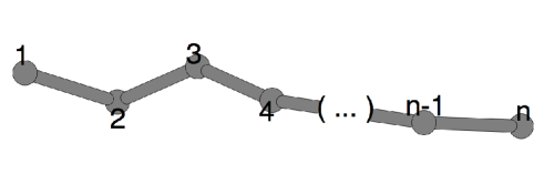
Figure 3.1: Numbering of the atoms in an open, single-branch chain.

If we only constrain bond lengths, the fact that only consecutive atoms participate of the same constraints allows us to simplify the notation with respect to eq. (2.7) and establish the following ordering for the constraints indices:

$$I(\alpha)=\alpha\ ,\quad I=1,\ldots,n-1\ ,$$ (3.3)

with

$$\sigma^{I(\alpha)}(\vec{x}_{\alpha},\vec{x}_{\alpha+1}):=(\vec{x}_{\alpha}-\vec{x}_{\alpha+1})^{2}-(a_{\alpha,\alpha+1})^{2}=0\ .$$ (3.4)

This choice results in a tridiagonal matrix $R$, whose only non-zero entries are those lying in the diagonal and its first neighbours. This is the only case for which an exact calculation of the Lagrange multipliers exists in the literature as far as we are aware [30].

3.2 Open, single-branch chain with constrained bond lengths and bond angles

The next step in complexity is to constrain the bond angles of the same linear chain that we discussed above. The atoms are ordered in the same way, as in fig. 3.1, and the trick to generate a banded matrix $R$ with minimal bandwidth is to alternatively index bond length constraints with odd numbers,

$$I(\alpha)=2\alpha-1=1,3,5,\ldots,2n-3\ ,\quad\mathrm{with}\quad\alpha=1,2,\ldots,n-1\ ,$$ (3.5)

and bond angle constraints with even ones,

$$J(\beta)=2\beta=2,4,6,\ldots,2n-4\ ,\quad\mathrm{with}\quad\beta=1,2,\ldots,n-2\ ,$$ (3.6)

where the regular pattern involving the atom indicies that participate of the same constraints has allowed again to use a lighter notation.

The constraints equations in this case are

$$\sigma^{I(\alpha)}(\vec{x}_{\alpha},\vec{x}_{\alpha+1})=(\vec{x}_{\alpha}-\vec{x}_{\alpha+1})^{2}-(a_{\alpha,\alpha+1})^{2}=0\ ,$$ (3.7a)

$$\sigma^{J(\beta)}(\vec{x}_{\beta},\vec{x}_{\beta+2})=(\vec{x}_{\beta}-\vec{x}_{\beta+2})^{2}-(a_{\beta,\beta+2})^{2}=0\ ,$$ (3.7b)

respectively, and, if this indexing is used, $R$ is a banded matrix where $m$ is 3 and 4 in consecutive rows and columns. Therefore, the mean $\langle m\rangle$ is 3.5, and the number of $\xi$ coefficients that have to be computed per row in the Gaussian elimination process is the same because the matrix contains no zeros that are filled.

A further feature of this system (and other systems where both bond lengths and bond angles are constrained) can be taken into account in order to reduce the computational cost of calculating Lagrange multipliers in a molecular dynamics simulation: A segment of the linear chain with constrained bond lengths and bond angles is represented in fig. 3.2, where the dashed lines correspond to the virtual bonds between atoms that, when kept constant, implement the constraints on bond angles (assuming that the bond lengths, depicted as solid lines, are also constrained).

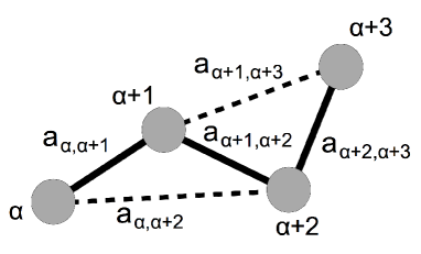
Figure 3.2: Segment of a single-branch chain with constrained bond lengths and bond angles. In solid line, the distances that have to be kept constant to constrain the former; in dashed line, those that have to be kept constant to constrain the latter.

Due to the fact that all these distances are constant, many of the entries of $R$ will remain unchanged during the molecular dynamics simulation. As an example, we can calculate

$$R_{2\alpha-1,2\alpha-2} = \frac{1}{m_{\alpha}}(\vec{x}_{\alpha}-\vec{x}_{\alpha+1})\cdot(\vec{x}_{\alpha}-\vec{x}_{\alpha+2})=\frac{a_{\alpha,\alpha+1}a_{\alpha,\alpha+2}}{m_{\alpha}}\cos\angle{(\alpha+1,\alpha,\alpha+2)}$$ (3.8)

$$= \frac{1}{2m_{\alpha}}(a_{\alpha,\alpha+1}^{2}+(a_{\alpha,\alpha+2})^{2}-a_{\alpha+1,\alpha+2}^{2})\ .$$

where we have used the law of cosines. The right-hand side does not depend on any time-varying objects (such as $\vec{x}_{\alpha}$), being made of only constant quantities. Therefore, the value of $R_{2\alpha-1,2\alpha-2}$ (and many other entries) needs not to be recalculated in every time step, which allows to save computation time in a molecular dynamics simulation.

3.3 Minimally branched molecules with constrained bond lengths

In order to incrementally complicate the calculations, we now turn to a linear molecule with only one atom connected to the backbone, such the one displayed in figure 3.3.

Figure 3.3: Numbering of the atoms in a minimally branched molecule.

The corresponding equations of constraint and the ordering in the indices that minimizes the bandwidth of the linear system are

$$\sigma^{1}=(\vec{x}_{1}-\vec{x}_{2})^{2}-a_{1,2}^{2}=0\ ,$$ (3.9a)

$$\sigma^{I(\alpha)}=(\vec{x}_{\alpha}-\vec{x}_{\alpha+1})^{2}-a_{\alpha,\alpha+1}^{2}=0\ ,\quad I(\alpha)=\alpha=2,4,6,\ldots,n-2\ ,$$ (3.9b)

$$\sigma^{J(\beta)}=(\vec{x}_{\beta}-\vec{x}_{\beta+2})^{2}-a_{\beta,\beta+2}^{2}=0\ ,\quad J(\beta)=\beta+1=3,5,7,\ldots,n-1\ ,$$ (3.9c)

where the trick this time has been to alternatively consider atoms in the backbone and atoms in the branches as we proceed along the chain.

The matrix $R$ of this molecule presents a semi-band width which is alternatively 2 and 1 in consecutive rows/columns, with average $\langle m\rangle=1.5$ and the same number of superdiagonal $\xi$ coefficients to be computed per row.

3.4 Alkanes with constrained bond lengths

The next molecular topology we will consider is that of an alkane (a familiy of molecules with a long tradition in the field of constraints [19]), i.e., a linear backbone with two 1-atom branches attached to each site (see fig. 3.4).

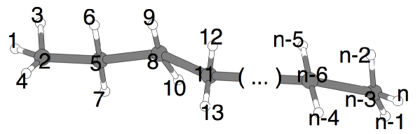
Figure 3.4: Numbering of the atoms in a model alkane chain.

The ordering of the constraints that minimizes the bandwidth of the linear system for this case is

$$\sigma^{1}(x)=(\vec{x}_{1}-\vec{x}_{2})^{2}-a_{1,2}^{2}=0\ ,$$ (3.10a)

$$\sigma^{I(\alpha)}(x)=(\vec{x}_{\alpha}-\vec{x}_{\alpha+3})^{2}-a_{\alpha+3,\alpha}^{2}=0\ ,\quad I(\alpha)=\alpha=2,5,8,\ldots,n-3\ ,$$ (3.10b)

$$\sigma^{J(\beta)}(x)=(\vec{x}_{\beta}-\vec{x}_{\beta+1})^{2}-a_{\beta+1,\beta}^{2}=0\ ,\quad J(\beta)=\beta+1=3,6,9,\ldots,n-2\ ,$$ (3.10c)

$$\sigma^{K(\gamma)}(x)=(\vec{x}_{\gamma}-\vec{x}_{\gamma+2})^{2}-a_{\gamma+2,\gamma}^{2}=0\ ,\quad K(\gamma)=\gamma+2=4,7,10,\ldots,n-1\ ,$$ (3.10d)

where the trick has been in this case to alternatively constrain the bond lengths in the backbone and those connecting the branching atoms to one side or the other. The resulting $R$ matrix require the calculation of 2 $\xi$ coefficients per row when solving the linear system.

3.5 Minimally branched molecules with constrained bond lengths and bond angles

If we want to additionally constrain bond angles in a molecule with the topology in fig. 3.3, the following ordering is convenient:

$$\sigma^{1}(x)=(\vec{x}_{1}-\vec{x}_{2})^{2}-a_{1,2}^{2}=0\ ,$$ (3.11a)

$$\sigma^{2}(x)=(\vec{x}_{2}-\vec{x}_{3})^{2}-a_{2,3}^{2}=0\ ,$$ (3.11b)

$$\sigma^{3}(x)=(\vec{x}_{1}-\vec{x}_{4})^{2}-a_{1,4}^{2}=0\ ,$$ (3.11c)

$$\sigma^{I(\alpha)}(x)=(\vec{x}_{\alpha}-\vec{x}_{\alpha+1})^{2}-a_{\alpha,\alpha+1}^{2}=0\ ,\quad I(\alpha)=2\alpha-2=4,8,12,\ldots,2n-4\ ,$$ (3.11d)

$$\sigma^{J(\beta)}(x)=(\vec{x}_{\beta}-\vec{x}_{\beta+2})^{2}-a_{\beta,\beta+2}^{2}=0\ ,\quad J(\beta)=2\beta+2=5,9,13,\ldots,2n-3\ ,$$ (3.11e)

$$\sigma^{K(\gamma)}(x)=(\vec{x}_{\gamma}-\vec{x}_{\gamma+1})^{2}-a_{\gamma,\gamma+1}^{2}=0\ ,\quad K(\gamma)=2\gamma-2=6,10,14,\ldots,2n-6\ ,$$ (3.11f)

$$\sigma^{L(\delta)}(x)=(\vec{x}_{\delta}-\vec{x}_{\delta+4})^{2}-a_{\delta,\delta+4}^{2}=0\ ,\quad L(\delta)=2\delta+3=7,11,15,\ldots,2n-5\ .$$ (3.11g)

This ordering produces 16 non-zero entries above the diagonal per each group of 4 rows in the matrix $R$ when making the calculations to solve the associated linear system. This is, we will have to calculate a mean of $16/4=4$ super-diagonal coefficients $\xi$ per row. When we studied the linear molecule with constrained bond lengths and bond angles, this mean was equal to $3.5$, so including minimal branches in the linear chain makes the calculations just slightly longer.

3.6 Alkanes with constrained bond lengths and bond angles

If we now want to add bond angle constraints to the bond length ones described in sec. 3.4 for alkanes, the following ordering produces a matrix $R$ with a low half-band width:

$$\sigma^{1}(x)=(\vec{x}_{2}-\vec{x}_{1})^{2}-a_{1,2}^{2}=0\ ,$$ (3.12a)

$$\sigma^{2}(x)=(\vec{x}_{3}-\vec{x}_{2})^{2}-a_{2,3}^{2}=0\ ,$$ (3.12b)

$$\sigma^{3}(x)=(\vec{x}_{4}-\vec{x}_{2})^{2}-a_{2,4}^{2}=0\ ,$$ (3.12c)

$$\sigma^{4}(x)=(\vec{x}_{5}-\vec{x}_{1})^{2}-a_{1,5}^{2}=0\ ,$$ (3.12d)

$$\sigma^{5}(x)=(\vec{x}_{5}-\vec{x}_{3})^{2}-a_{3,5}^{2}=0\ ,$$ (3.12e)

$$\sigma^{6}(x)=(\vec{x}_{5}-\vec{x}_{4})^{2}-a_{4,5}^{2}=0\ ,$$ (3.12f)

$$\sigma^{I(\alpha)}(x)=(\vec{x}_{\alpha}-\vec{x}_{\alpha+3})^{2}-a_{\alpha,\alpha+3}^{2}=0\ ,\quad I(\alpha)=2\alpha+3=7,13,19,\ldots,2n-3\ ,$$ (3.12g)

$$\sigma^{J(\beta)}(x)=(\vec{x}_{\beta}-\vec{x}_{\beta+1})^{2}-a_{\beta,\beta+1}^{2}=0\ ,\quad J(\beta)=2\beta-2=8,14,20,\ldots,2n-8\ ,$$ (3.12h)

$$\sigma^{K(\gamma)}(x)=(\vec{x}_{\gamma}-\vec{x}_{\gamma+2})^{2}-a_{\gamma,\gamma+2}^{2}=0\ ,\quad K(\gamma)=2\gamma-1=9,15,21,\ldots,2n-7\ ,$$ (3.12i)

$$\sigma^{L(\delta)}(x)=(\vec{x}_{\delta}-\vec{x}_{\delta+6})^{2}-a_{\delta,\delta+6}^{2}=0\ ,\quad L(\delta)=2\delta+6=10,16,22,\ldots,2n-6\ ,$$ (3.12j)

$$\sigma^{M(\epsilon)}(x)=(\vec{x}_{\epsilon}-\vec{x}_{\epsilon+2})^{2}-a_{\epsilon,\epsilon+2}^{2}=0\ ,\quad M(\epsilon)=2\epsilon-1=11,17,23,\ldots,2n-5\ ,$$ (3.12k)

$$\sigma^{N(\zeta)}(x)=(\vec{x}_{\zeta}-\vec{x}_{\zeta+1})^{2}-a_{\zeta,\zeta+1}^{2}=0\ ,\quad N(\zeta)=2\zeta-2=12,18,24,\ldots,2n-4\ .$$ (3.12l)

In this case, the average number of $\xi$ coefficients to be calculated per row is approximately 5.7.

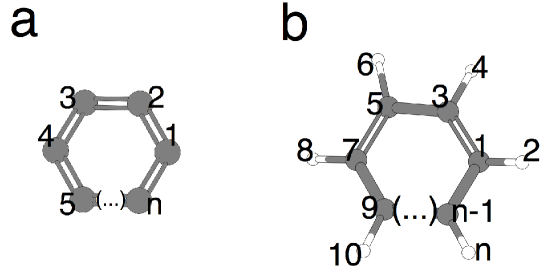
Figure 3.5: Numbering of the atoms for cyclic molecules: a) without branches; b) minimally branched.

3.7 Cyclic chains

If we have cycles in our molecules, the indexing of the constraints is only slightly modified with respect to the open cases in the previous sections. For example, if we have a single-branch cyclic topology, such as the one displayed in fig. 3.5a, the ordering of the constraints is the following:

$$\sigma^{I(\alpha)}(x)=(\vec{x}_{\alpha}-\vec{x}_{\alpha+1})^{2}-(a_{\alpha,\alpha+1})^{2}=0\ ,\quad I(\alpha)=1,\ldots,n-1=\alpha\ ,$$ (3.13a)

$$\sigma^{n}(x)=(\vec{x}_{1}-\vec{x}_{n})^{2}-(a_{1,n})^{2}=0\ .$$ (3.13b)

These equations are the same as those in 3.1, plus a final constraint corresponding to the bond which closes the ring. These constraints produce a matrix $R$ where only the diagonal entries, its first neighbours, and the entries in the corners ($R_{1,n}$ and $R_{n,1}$) are non-zero. In this case, the associated linear system in eq. (2.6) can also be solved in $O(N_{c})$ operations, as we discuss in [18]. In general, this is also valid whenever $R$ is a sparse matrix with only a few non-zero entries outside of its band, and therefore we can apply the technique introduced in this work to molecular topologies containing more than one cycle.

The ordering of the constraints and the resulting linear systems for different cyclic species, such as the one depicted in fig. 3.5b, can be easily constructed by the reader using the same basic ideas.

3.8 Proteins

As we discussed in sec. 1, proteins are one of the most important families of molecules from the biological point of view: Proteins are the nanomachines that perform most of the complex tasks that need to be done in living organisms, and therefore it is not surprising that they are involved, in one way or another, in most of the diseases that affect animals and human beings. Given the efficiency and precision with which proteins carry out their missions, they are also being explored from the technological point of view. The applications of proteins even outside the biological realm are many if we could harness their power [1], and molecular dynamics simulations of great complexity and scale are being done in many laboratories around the world as a tool to understand them [31, 4, 32].

Proteins present two topological features that simplify the calculation of the Lagrange multipliers associated to constraints imposed on their degrees of freedom:

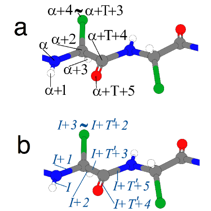
Figure 3.6: Scheme of the residue of a protein. a) Numbering of the atoms; $\alpha$ represents the first numbered atom in each residue (the amino nitrogen) and $T$ is the number of atoms in the side chain. b) Indexing of the bond length constraints; $I$ denotes the index of the first constraint imposed on the residue (the N-H bond length) and $T^{\prime}$ is the variable number of constraints imposed on the side chain.

• They are linear polymers, consisting of a backbone with short (17 atoms at most) groups attached to it [1]. This produces a banded matrix $R$, thus allowing the solution of the associated linear problem in $O(N_{c})$ operations. Even in the case that disulfide bridges, or any other covalent linkage that disrupts the linear topology of the molecule, exist, the solution of the problem can still be found efficiently if we recall the ideas discussed in sec. 3.7.

• The monomers that typically make up these biological polymers, i.e., the residues associated to the proteinogenic aminoacids, are only 20 different molecular structures. Therefore, it is convenient to write down explicitly one block of the $R$ matrix for each known monomer, and to build the $R$ matrix of any protein simply joining together the precalculated blocks associated to the corresponding residues the protein consists of.

The structure of a segment of the backbone of a protein chain is depicted in fig. 3.6. The green spheres represent the side chains, which are the part of the amino acid residue that can differ from one monomer to the next, and which usually consist of several atoms: from 1 atom in the case of glycine to 17 in arginine or tryptophan. In fig. 3.6a, we present the numbering of the atoms, which will support the ordering of the constraints, and, in fig. 3.6b, the indexing of the constraints is presented for the case in which only bond lengths are constrained (the bond lengths plus bond angles case is left as an exercise for the reader).

Using the same ideas and notation as in the previous sections and denoting by $R_{\mathcal{M}}$ the block of the matrix $R$ that corresponds to a given amino acid residue $\mathcal{M}$, with $\mathcal{M}=1,\ldots,\mathcal{N}_{\mathcal{R}}$, we have that, for the monomer dettached of the rest of the chain,

$$R_{\mathcal{M}}=\left(\begin{array}[]{ccc|lcr|ccc}\Omega&\omega&&&&&&&\\ \omega&\Omega&\omega&\omega&&&\omega&&\\ &\omega&\Omega&\omega&&&\omega&&\\ \hline\cr&\omega&\omega&&&&\omega&&\\ &&&&S&&&&\\ &&&&&&&&\\ \hline\cr&\omega&\omega&\omega&&&\Omega&\omega&\omega\\ &&&&&&\omega&\Omega&\omega\\ &&&&&&\omega&\omega&\Omega\\ \end{array}\right)\ ,$$ (3.14)

where the explicit non-zero entries are related to the constraints imposed on the backbone and $S$ denotes a block associated to those imposed on the bonds that belong to the different sidechains. The dimension of this matrix is $T^{\prime}+6$ and the maximum possible semi-band width is 12 for the bulkiest residues.

A protein’s global matrix $R$ has to be built by joining together blocks like the one above, and adding the non-zero elements related to the imposition of constraints on bond lengths that connect one residue with the next. These extra elements are denoted by $\omega_{C}$ and a general scheme of the final matrix is shown in fig. 3.7.

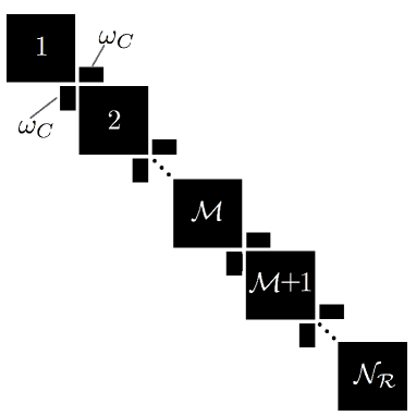
Figure 3.7: Scheme of the matrix $R$ for a protein molecule with $\mathcal{N_{R}}$ residues. In black, we represent the potentially non-zero entries, and each large block in the diagonal is given by (2.4c).

The white regions in this scheme correspond to zero entries, and we can easily check that the matrix is banded. In fact, if each one of the diagonal blocks is constructed conveniently, they will contain many zeros themselves and the bandwidth can be reduced further. The size of the $\omega_{C}$ blocks will usually be much smaller than that of their neighbour diagonal blocks. For example, in the discussed case in which we constrain all bond lengths, $\omega_{C}$ are $1\times 2$ (or $2\times 1$) blocks, and the diagonal blocks size is between $7\times 7$ (glycine) and $25\times 25$ (tryptophan).

3.9 Nucleic acids

Nucleic acids are another family of very important biological molecules that can be tackled with the techniques described in this work. DNA and RNA, the two subfamilies of nucleic acids, consist of linear chains made up of a finite set of monomers (called ‘bases’). This means that they share with proteins the two features mentioned in the previous section and therefore the Lagrange multipliers associated to the imposition of constraints on their degrees of freedom can be efficiently computed using the same ideas. It is worth mentioning that DNA typically appears in the form of two complementary chains whose bases form hydrogen-bonds. Since these bonds are much weaker than a covalent bond, imposing bond length constraints on them such as the ones in eq. (2.7) would be too unrealistic for many practical purposes,

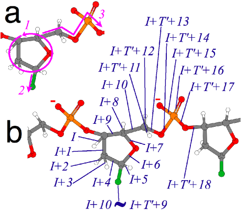
Figure 3.8: Constraints indexing of a DNA nucleotide a) General order to be followed. b) Indexing of the bond length constraints; $I$ denotes the index of the first constraint imposed on the nucleotide and $T^{\prime}$ is the variable number of constraints imposed on the bonds in the base.

In fig. 3.8, and following the same ideas as in the previous section, we propose a way to index the bond length constraints of a DNA strand which produces a banded matrix $R$ of low bandwidth. Green spheres represent the (many-atom) bases (A, C, T or G), and the general path to be followed for consecutive constraint indices is depicted in the upper left corner: first the sugar ring, then the base and finally the rest of the nucleotide, before proceeding to the next one in the chain.

This ordering translates into the following form for the block of $R$ corresponding to one single nucleotide dettached from the rest of the chain:

$$R_{\mathcal{M}}=\left(\begin{array}[]{ccc|ccc|ccc}&&&&&&&&\\ &R_{\mathcal{M}}^{1,1}&&&R_{\mathcal{M}}^{1,2}&&&R_{\mathcal{M}}^{1,3}&\\ &&&&&&&&\\ \hline\cr&&&&&&&&\\ &R_{\mathcal{M}}^{2,1}&&&S&&&&\\ &&&&&&&&\\ \hline\cr&&&&&&&&\\ &R_{\mathcal{M}}^{3,1}&&&&&&R_{\mathcal{M}}^{3,3}&\\ &&&&&&&&\\ \end{array}\right)\ ,$$ (3.15)

where $S$ is the block associated to the constraints imposed on the bonds that are contained in the base, $R_{\mathcal{M}}^{1,2}$, $R_{\mathcal{M}}^{1,3}$, $R_{\mathcal{M}}^{2,1}$, and $R_{\mathcal{M}}^{3,1}$ are very sparse rectangular blocks with only a few non-zero entries in them, and the form of the diagonal blocks associated to the sugar ring and backbone constraints is the following:

$$R_{\mathcal{M}}^{1,1} =\left(\begin{array}[]{cccccccccc}\Omega&\omega&&&&&&&&\omega\\ \omega&\Omega&\omega&\omega&\omega&&&&&\\ &\omega&\Omega&\omega&\omega&&&&&\\ &\omega&\omega&\Omega&\omega&&&&&\\ &\omega&\omega&\omega&\Omega&\omega&\omega&&&\\ &&&&\omega&\Omega&\omega&&&\\ &&&&\omega&\omega&\Omega&\omega&&\\ &&&&&&\omega&\Omega&\omega&\omega\\ &&&&&&&\omega&\Omega&\omega\\ \omega&&&&&&&\omega&\omega&\Omega\\ \end{array}\right)\ ,$$ (3.16k)

$$R_{\mathcal{M}}^{1,1} =\left(\begin{array}[]{ccccccccc}\Omega&\omega&\omega&\omega&&&&&\\ \omega&\Omega&\omega&\omega&&&&&\\ \omega&\omega&\Omega&\omega&&&&&\\ \omega&\omega&\omega&\Omega&\omega&&&&\\ &&&\omega&\Omega&\omega&\omega&\omega&\\ &&&&\omega&\Omega&\omega&\omega&\\ &&&&\omega&\omega&\Omega&\omega&\\ &&&&\omega&\omega&\omega&\Omega&\omega\\ &&&&&&&\omega&\Omega\\ \end{array}\right)\ .$$ (3.16u)

Analagously to the case of proteins, as many blocks as those in eq. (3.15) as nucleotides contains a given DNA strand have to be joined to produce the global matrix $R$ of the whole molecule, together with the $\omega_{C}$ blocks associated to the constraints on the bonds that connect the different monomers. In fig. 3.9, a scheme of this global matrix is depicted and we can appreciate that it indeed banded. The construction of the matrix $R$ for a RNA molecule should follow the same steps and the result will be very similar.

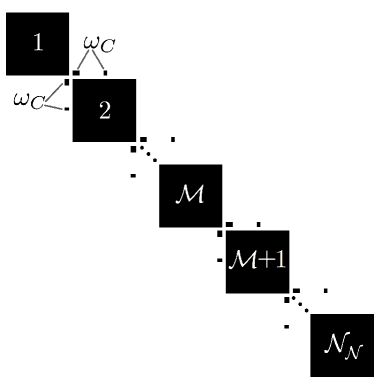
Figure 3.9: Scheme of the matrix $R$ for a DNA molecule with $\mathcal{N_{N}}$ nucleotides. In black, we represent the potentially non-zero entries, and each large block in the diagonal is given by (3.15).

4 Numerical calculations

In this section, we apply the efficient technique introduced in this work to a series of polyalanine molecules in order to calculate the Lagrange multipliers when bond length constraints are imposed. We also compare our method, both in terms of accuracy and numerical efficiency, to the traditional inversion of the matrix $R$ without taking into account its banded structure.

We used the code Avogadro [33] to build polyalanine chains of $N_{\mathrm{res}}=$2, 5, 12, 20, 30, 40, 50, 60, 80, 90 and 100 residues, and we chose their initial conformation to be approximately an alpha helix, i.e., with the values of the Ramachandran angles in the backbone $\phi=-60^{o}$ and $\psi=-40^{o}$ [1]. Next, for each of these chains, we used the molecular dynamics package AMBER [34] to produce the atoms positions ($x$), velocities ($v$) and external forces ($F$) needed to calculate the Lagrange multipliers (see sec. 2) after a short equilibration molecular dynamics simulations. We chose to constrain all bond lengths, but our method is equally valid for any other choice, as the more common constraining only of bonds that involve hydrogens.

In order to produce reasonable final conformations, we repeated the following process for each of the chains:

• Solvation with explicit water molecules.

• Minimization of the solvent positions holding the polypeptide chain fixed (3,000 steps).

• Minimization of all atoms positions (3,000 steps).

• Thermalization: changing the temperature from 0 K to 300 K during 10,000 molecular dynamics steps.

• Stabilization: 20,000 molecular dynamics steps at a constant temperature of 300 K.

• Measurement of $x$, $v$ and $F$.

Neutralization is not necessary, because our polyalanine chains are themselves neutral. In all calculations we used the force field described in [35], chose a cutoff for Coulomb interactions of 10 Å and a time step equal to 0.002 ps, and impose constraints on all bond lengths as mentioned. In the thermostated steps, we used Langevin dynamics with a collision frequency of 1 ps^-1.

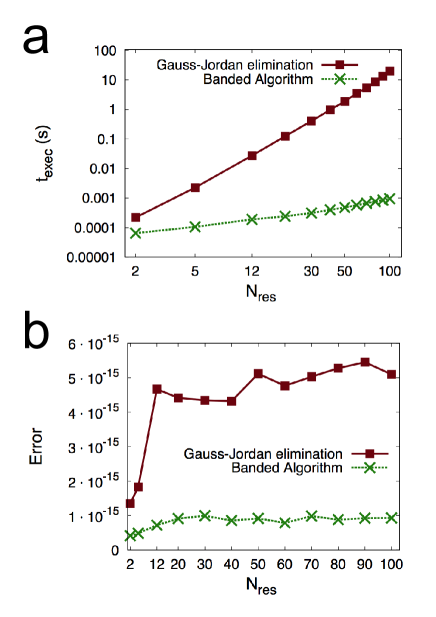
Figure 4.1: Comparison of a) numerical complexity and b) accuracy between a traditional Gauss-Jordan solver (solid line) and the banded algorithm described in this work (dashed line), for the calculation of the Lagrange multipliers on a series of polyalanine chains as a function of their number of residues $N_{\mathrm{res}}$.

Using the information obtained and the indexing of the constraints described in this work, we constructed the matrix $R$ and the vector $o$ and proceeded to find the Lagrange multipliers using eq. (2.6). Since (2.6) is a linear problem, one straightforward way to solve is to use traditional Gauss-Jordan elimination or LU factorization [17, 36]. But these methods have a drawback: they scale with the cube of the size of the system. I.e., if we imposed $N_{c}$ constraints on our system (and therefore we needed to obtain $N_{c}$ Lagrange multipliers), the number of floating point operations that these methods would require is proportional to $N_{c}^{3}$. However, as we showed in the previous sections, the fact that many biological molecules, and proteins in particular, are essentially linear, allows to index the constraints in such a way that the matrix $R$ in eq. (2.6) is banded and use different techniques for solving the problem which require only $O(N_{c})$ floating point operations [18].

$N_{\mathrm{res}}$	Gauss-Jordan	Banded Alg.	Gauss-Jordan	Banded Alg.
	Error	Error	$t_{\mathrm{exec}}$ (s)	$t_{\mathrm{exec}}$ (s)
2	$1.355\cdot 10^{-15}$	$4.193\cdot 10^{-16}$	$2.185\cdot 10^{-4}$	$6.500\cdot 10^{-5}$
5	$1.829\cdot 10^{-15}$	$4.897\cdot 10^{-16}$	$2.263\cdot 10^{-3}$	$1.059\cdot 10^{-4}$
12	$4.660\cdot 10^{-15}$	$7.244\cdot 10^{-16}$	$2.733\cdot 10^{-2}$	$1.897\cdot 10^{-4}$
20	$4.413\cdot 10^{-15}$	$9.160\cdot 10^{-16}$	0.1239	$2.407\cdot 10^{-4}$
30	$4.340\cdot 10^{-15}$	$9.975\cdot 10^{-16}$	0.4075	$3.115\cdot 10^{-4}$
40	$4.318\cdot 10^{-15}$	$8.591\cdot 10^{-16}$	0.9669	$3.975\cdot 10^{-4}$
50	$5.113\cdot 10^{-15}$	$9.209\cdot 10^{-16}$	1.877	$4.811\cdot 10^{-4}$
60	$4.761\cdot 10^{-15}$	$7.906\cdot 10^{-16}$	3.457	$5.751\cdot 10^{-4}$
70	$5.026\cdot 10^{-15}$	$9.868\cdot 10^{-16}$	5.381	$6.664\cdot 10^{-4}$
80	$5.271\cdot 10^{-15}$	$8.843\cdot 10^{-16}$	8.633	$7.605\cdot 10^{-4}$
90	$5.448\cdot 10^{-15}$	$9.287\cdot 10^{-16}$	13.42	$8.527\cdot 10^{-4}$
100	$5.091\cdot 10^{-15}$	$9.342\cdot 10^{-16}$	19.69	$9.484\cdot 10^{-4}$

Table 1: Comparison of numerical complexity and accuracy between a traditional Gauss-Jordan solver and the banded algorithm described in this work, for the calculation of the Lagrange multipliers on a series of polyalanine chains as a function of their number of residues $N_{\mathrm{res}}$.

In fig. 4.1 and table 1, we compare both the accuracy and the execution time of the two different methods: Gauss-Jordan elimination [36], and the banded recursive solution advocated here and made possible by the appropriate indexing of the constraints. The calculations have been run on a Mac OS X laptop with a 2.26 GHz Intel Core 2 Duo processor, and the errors were measured using the normalized deviation of $R\lambda$ from $-o$. I.e., if we denote by $\lambda$ the solution provided by the numerical method,

$$\mathrm{Error}:=\frac{\sum_{I=1}^{N_{c}}\left|\sum_{J=1}^{N_{c}}R_{IJ}\lambda_{J}+o_{I}\right|}{\sum_{I=1}^{N_{c}}|\lambda_{I}|}\ .$$ (4.1)

From the obtained results, we can see that both methods produce an error which is very small (close to machine precision), being the accuracy of the banded algorithm advocated in this work slightly higher. Regarding the computational cost, as expected, the Gauss-Jordan method presents an effort that approximately scales with the cube of the number of constraints $N_{c}$ (which is approximately proportional to $N_{\mathrm{res}}$), while the banded technique allowed by the particular structure of the matrix $R$ follows a rather accurate lineal scaling. Although it is typical that, when two such different behaviours meet, there exists a range of system sizes for which the method that scales more rapidly is faster and then, at a given system size, a crossover takes place and the slower scaling method becomes more efficient from there on, in this case, and according to the results obtained, the banded technique is less time-consuming for all the explored molecules, and the crossover should exist at a very small system size (if it exists at all). This is very relevant for any potential uses of the methods introduced in this work.

5 Conclusions

We have shown that, if we are dealing with typical biological polymers, whose covalent connectivity is that of essentially linear objects, the Lagrange multipliers that need to be computed when $N_{c}$ constraints are imposed on their internal degrees of freedom (such as bond lengths, bond angles, etc.) can be obtained in $O(N_{c})$ steps as long as the constraints are indexed in a convenient way and banded algorithms are used to solve the associated linear system of equations. This path has been traditionally regarded as too costly in the literature [19, 20, 21, 22, 23, 24], and, therefore, our showing that it can be implemented efficiently could have profound implications in the design of future molecular dynamics algorithms.

Since the field of imposition of constraints in moleculary dynamics simulations is dominated by methods that cleverly achieve that the system exactly stays on the constrained subspace as the simulation proceeds by not calculating the exact Lagrange multipliers, but a modification of them instead [19, 37], we are aware that the application of the new techniques introduced here is not a direct one. However, we are confident that the low cost of the new method and its close relationship with the problem of constrained dynamics could prompt many advances, some of which are already being pursued in our group. Among the most promising lines, we can mention a possible improvement of the SHAKE method [19] by the use of the exact Lagrange multipliers as a guess for the iterative procedure that constitutes its most common implementation. Also, we are studying the possibility of solving the linear problems that appear either in a different implementation of SHAKE (mentioned in the original work too [19]) or in the LINCS method [37], and which are defined by matrices which are different from but related to the matrix $R$ introduced in this work, being also banded if an appropriate indexing of the constraints is used. Finally, we are exploring an extension of the ideas introduced here to the calculation not only of the Lagrange multipliers but also of their time derivatives, to be used in higher order integrators than Verlet.

References

- [1] P. Echenique, Introduction to protein folding for physicists, Contemp. Phys. 48 (2007) 81–108.
- [2] H. Cedar and Y. Bergman, Linking DNA methylation and histone modification: patterns and paradigms, Nat. Rev. Genet. 10 (2009) 295–-304.
- [3] S. Piana, K. Sarkar, K. Lindorff-Larsen, G. Minghao, M. Gruebele, and D. E. Shaw, Computational Design and Experimental Testing of the Fastest-Folding β-Sheet Protein, J. Mol. Biol. 405,1 (2011) 43–48.
- [4] D. E. Shaw, R. Ron O. Dror, J. Salmon, J. Grossman, K. Mackenzie, J. Bank, C. Young, B. Batson, K. Bowers, E. Edmond Chow, M. Eastwood, D. Ierardi, J. John L. Klepeis, J. Jeffrey S. Kuskin, R. Larson, K. Kresten Lindorff-Larsen, P. Maragakis, M. M.A., S. Piana, S. Yibing, and B. Towles, Millisecond-Scale Molecular Dynamics Simulations on Anton, In Proceedings of the ACM/IEEE Conference on Supercomputing (SC09), ACM Press, New York, (2009) .
- [5] W. A. de Jong, E. Bylaska, N. Govind, C. L. Janssen, K. Kowalski, T. Müller, I. Nielsen, H. van Dam, V. Veryazov, and R. Lindh, Utilizing high performance computing for chemistry: parallel computational chemistry, PCCP 12 (2010) 6896–-6920.
- [6] J. C. Phillips, R. Braun, W. Wei, J. Gumbart, E. Tajkhorshid, E. Villa, C. Chipot, R. D. Skeel, L. Kalé, and K. Schulten, Scalable molecular dynamics with NAMD, JCC 26,16 (2005) 1781–1802.
- [7] D. A. Pearlman, D. A. Case, J. W. Caldwell, W. R. Ross, T. E. Cheatham III, S. DeBolt, D. Ferguson, G. Seibel, and P. Kollman, AMBER, a computer program for applying molecular mechanics, normal mode analysis, molecular dynamics and free energy calculations to elucidate the structures and energies of molecules, Comp. Phys. Commun. 91 (1995) 1–41.
- [8] P. Gonnet, J. H. Walther, and P. Koumoutsakos, Theta SHAKE: An extension to SHAKE for the explicit treatment of angular constraints, Journal of Chemical Physics 180 (2009) 360–364.
- [9] L. Verlet, Computer “experiments” on classical fluids. I. Thermodynamical properties of Lennard-Jones molecules, Phys. Rev. 159 (1967) 98–103.
- [10] D. Frenkel and B. Smit, Understanding molecular simulations: From algorithms to applications, Academic Press, Orlando FL, 2nd edition, 2002.
- [11] K. A. Feenstra, B. Hess, and H. J. C. Berendsen, Improving Efficiency of Large Time-scale Molecular Dynamics Simulations of Hydrogen-rich Systems, J. Comput. Chem. 20 (1999) 786–798.
- [12] P. Eastman and V. S. Pande, Constant Constraint Matrix Approximation: A Robust, Parallelizable Constraint Method for Molecular Simulations, J. Chem. Theory Comput. 6 (2) (2010) 434–437.
- [13] A. K. Mazur, Hierarchy of Fast Motions in Protein Dynamics, J. Phys. Chem. B 102 (1998) 473–479.
- [14] P. Echenique, I. Calvo, and J. L. Alonso, Quantum mechanical calculation of the effects of stiff and rigid constraints in the conformational equilibrium of the Alanine dipeptide, J. Comput. Chem. 27 (2006) 1748–1755.
- [15] W. F. Van Gunsteren and M. Karplus, Effects of constraints on the dynamics of macromolecules, Macromolecules 15 (1982) 1528–1544.
- [16] E. Barth, K. Kuczera, B. Leimkuhler, and R. D. Skeel, Algorithms for constrained molecular dynamics, J. Comput. Phys. 16 (10) (1995) 1192–1209.
- [17] H. Goldstein, C. Poole, and J. Safko, Classical Mechanics, Addison-Wesley, 3rd edition, 2002.
- [18] P. García-Risueño and P. Echenique, Linearly scaling direct method for accurately inverting sparse banded matrices, Submitted (2010) .
- [19] J. P. Ryckaert, G. Ciccotti, and H. J. C. Berendsen, Numerical integration of the Cartesian equations of motion of a system with constraints: Molecular dynamics of n-alkanes, J. Comput. Phys. 23 (1977) 327–341.
- [20] J. L. M. Dillen, On the use of constraints in molecular mechanics. II. The Lagrange multiplier method and non-full-matrix Newton-Raphson minimization, J. Comput. Chem. 8,8 (1987) 1099–1103.
- [21] G. Ciccotti and J. P. Ryckaert, Molecular dynamics simulation of rigid molecules, Comput. Phys. Rep. 4 (1986) 345–392.
- [22] V. Krautler, W. F. Van Gunsteren, and P. H. Hunenberger, A fast SHAKE Algorithm to Solve Distance Constraint Equations for Small Molecules in Molecular Dynamics Simulations, J. Comput. Chem. 22 (2001) 501–508.
- [23] P. Gonnet, P-SHAKE: a quadratically convergent SHAKE in O(n squared), J. Chem. Phys. 220 (2006) 740–750.
- [24] M. Mazars, Holonomic Constraints: An Analytical Result, J. Phys. A: Math. Theor. 40, 8 (2007) 1747–1755.
- [25] R. Featherstone, A Divide-and-Conquer Articulated-Body Algorithm for Parallel O(log(n)) Calculation of Rigid-Body Dynamics. Part 1: Basic Algorithm, Int. J. of Rob. Res. 18 (1999) 867.
- [26] D.-S. Bae and E. Haug, A recursive formulation for constrained mechanical system dynamics: Part I. Open loop systems., Mech. Struct. and Mach. 15 (1987) 359–382.
- [27] K. Lee, Y. Wang, and G. Chirikjian, O(n) mass matrix inversion for serial manipulators and polypeptide chains using Lie derivatives, Robotica 25 (2007) 739–750.
- [28] M. Henneux and C. Teitelboim, Quantization of gauge fields, Princeton Univesity Press, 1992.
- [29] P. Echenique and J. L. Alonso, Definition of Systematic, Approximately Separable and Modular Internal Coordinates (SASMIC) for macromolecular simulation, J. Comput. Chem. 27 (2006) 1076–1087.
- [30] M. Mazars, Holonomic constraints, an analytical result, J. Phys. A: Math. Theor. 49 (2007) 1747–1755.
- [31] D. Lucent, V. Vishal, and V. S. Pande, Protein folding under confinement: A role for solvent, Proc. Natl. Acad. Sci. USA 104,25 (2007) 10430–-10434.
- [32] P. L. Freddolino and K. Schulten, Common Structural Transitions in Explicit-Solvent Simulations of Villin Headpiece Folding, Biophys. J. 97 (2009) 2338–2347.
- [33] Avogadro: an open-source molecular builder and visualization tool. Version 1.0.1 (2010) , \urlhttp://avogadro.openmolecules.net/.
- [34] D. A. Case, T. Darden, T. E. Cheatham, C. Simmerling, W. Junmei, D. R. E., R. Luo, K. M. Merz, M. A. Pearlman, M. Crowley, R. Walker, Z. Wei, W. Bing, S. Hayik, A. Roitberg, G. Seabra, W. Kim, F. Paesani, W. Xiongwu, V. Brozell, S. Tsui, H. Gohlke, Y. Lijiang, T. Chunhu, J. Mongan, V. Hornak, P. Guanglei, C. Beroza, D. H. Mathews, C. Schafmeister, W. S. Ross, and P. A. Kollman, AMBER 9 User’s Manual, University of California: San Francisco (2006) .
- [35] D. Yong, W. Chun, S. Chowdhury, M. C. Lee, X. Guoming, Z. Wei, Y. Rong, P. Cieplak, R. Luo, L. Taisung, J. Caldwell, J. Wang, and P. Kollman, A point-charge force field for molecular mechanics simulations of pro- teins based on condensed-phase quantum mechanical calculations, J. Comput. Chem. 24 (2003) 1999–2012.
- [36] W. H. Press, S. A. Teukolsky, W. T. Vetterling, and B. P. Flannery, Numerical recipes. The art of scientific computing, Cambridge University Press, New York, 3nd edition, (2007).
- [37] B. Hess, H. Bekker, H. J. C. Berendsen, and J. G. E. M. Fraaije, LINCS: A Linear constraint solver for molecular simulations, J. Comput. Chem. 18 (1997) 1463–1472.