Phase diagram for a Cubic Consistent-Q Interacting Boson Model Hamiltonian: signs of triaxiality

Abstract

An extension of the Consistent-Q formalism for the Interacting Boson Model that includes the cubic $(\hat{Q}\times\hat{Q}\times\hat{Q})^{(0)}$ term is proposed. The potential energy surface for the cubic quadrupole interaction is explicitly calculated within the coherent state formalism using the complete ($\chi-$dependent) expression for the quadrupole operator. The Q-cubic term is found to depend on the asymmetry deformation parameter $\gamma$ as a linear combination of $\cos{(3\gamma)}$ and $\cos^{2}{(3\gamma)}$ terms, thereby allowing for triaxiality. The phase diagram of the model in the large N limit is explored, it is described the order of the phase transition surfaces that define the phase diagram, and moreover, the possible nuclear equilibrium shapes are established. It is found that, contrary to expectations, there is only a very tiny region of triaxiality in the model, and that the transition from prolate to oblate shapes is so fast that, in most cases, the onset of triaxiality might go unnoticed.

I Introduction

The quadrupole operator plays a central role in Nuclear Physics because it is essential in the description of nuclear deformation, in the calculation of energy terms and in the evaluation of electromagnetic quadrupole transitions and moments Bohr75 . Its presence is also of key importance within the Interacting Boson Model (IBM) ibm ; GK , where its components are defined, in terms of $s$ and $d$ bosons, as

$$\hat{Q}_{\mu}=[d^{\dagger}\tilde{s}+s^{\dagger}\tilde{d}]^{(2)}_{\mu}+\chi[d^{\dagger}\tilde{d}]^{(2)}_{\mu}.$$ (1)

Various relevant operators (including scalar terms in the Hamiltonian or the $E2$ electromagnetic transition operator) are usually built from $\hat{Q}$ by appropriate tensor couplings. Within the IBM a useful and, at the same time, extremely simple Hamiltonian is the one of the Consistent-Q formalism (CQF) introduced some time ago by D.D. Warner and R.F. Casten Warn83 . This model Hamiltonian is formed by a one body monopole term, proportional to the number of $d$ bosons, plus a quadrupole-quadrupole interaction among bosons. The CQF Hamiltonian can generate spherical, deformed axially symmetric as well as deformed $\gamma-$unstable potential energy surfaces ibm . It was noted ibm that for a general s-d IBM Hamiltonian including up to two body terms, triaxial shapes are forbidden (please, note that triaxiallity can be obtained with up to two-body terms if g-bosons are included sdgPiet ). Within the standard s-d IBM several authors have shown (for example in Refs. Hey ; ThJE ; Garc00a ; Garc00b ; ibm , in ch. 6 of Ref. BB , ch. 2.2 of Ref. Bon and in Ref. Jolo04 ) that the triaxiality can be successfully introduced by adding three-body terms of the type $[d^{\dagger}d^{\dagger}d^{\dagger}]^{(L)}\cdot[\tilde{d}\tilde{d}\tilde{d}]^{(L)}$. These terms, together with a CQF Hamiltonian, generate a relatively broad region of triaxiality in the parameter space of the Hamiltonian. Although this is a valid way of generating triaxiality, it is not completely satisfactory because there is a priori no reason to invoke such terms and moreover one moves away of the desirable simplicity of the CQF framework. An alternative is to use higher order terms in $\hat{Q}$ as, for instance, the cubic $(\hat{Q}\times\hat{Q}\times\hat{Q})^{(0)}$ interaction. The explicit expression for the cubic order interaction reads,

$$(\hat{Q}\times\hat{Q}\times\hat{Q})^{(0)}=\sum_{\nu,\mu}\langle 2\nu 2-\nu|00\rangle\langle 2\mu 2(\nu-\mu)|2\nu\rangle\hat{Q}_{\mu}\hat{Q}_{\nu-\mu}\hat{Q}_{-\nu},$$ (2)

where $\langle....|..\rangle$ stands for Clebsh-Gordan coefficients. Here three quadrupole operators (with rank-2 tensorial properties) are coupled to give a scalar term. This operator couples states with $\Delta\tau=3$ as well as $\Delta\tau=1$, where $\tau$ is the $O(5)$ seniority quantum number.

Several studies have been carried out for disentangling the properties of Hamiltonians containing $\hat{Q}\times\hat{Q}\times\hat{Q}$ terms. On the one hand, P. Van Isacker piet has studied the tensorial properties of the $\hat{Q}\times\hat{Q}\times\hat{Q}$ operator, within the IBM, and has shown that, even with $\chi=0$, this cubic operator can give spectra and band structures that are qualitatively similar to those usually associated with a SU(3) type of symmetry (axial rotor). On the other hand, Rowe and Thiamova RoTi have recently investigated the spectrum generated by using the following Hamiltonian

$$\hat{H}=\hat{\Lambda}+k(\hat{Q}\times\hat{Q}\times\hat{Q})^{(0)}\;,$$ (3)

where $\Lambda$ is the Casimir operator of $O(5)$, reaching similar conclusions to those of P. Van Isacker: the spectrum obtained by increasing the strength of the cubic term with $\chi=0$ displays the properties of an axially symmetric rotor. In their paper and, more recently in Ref. Thi , it is shown that the contraction of the O(6) algebra indicates that $\cos{(3\gamma)}$ is an image of the cubic term and therefore the only possible stable shapes are axially deformed. Following this reasoning, a quadratic term in the $\hat{Q}$ cubic scalar, i.e. $(\hat{Q}\times\hat{Q}\times\hat{Q})^{(0)}\cdot(\hat{Q}\times\hat{Q}\times\hat{Q})^{(0)}$, is necessary to generate potential energy terms displaying a $\cos^{2}{(3\gamma)}$ behavior. While this is most certainly true with their assumption on the form of the quadrupole operator ($\hat{Q}_{\mu}=[d^{\dagger}s+s^{\dagger}\tilde{d}]^{(2)}_{\mu}$, i.e. $\chi=0$), we find by explicit calculation that a term quadratic in the cosine is already present in the matrix elements of the $(\hat{Q}\times\hat{Q}\times\hat{Q})^{(0)}$ operator alone, if one includes the $\chi$ dependent term in the definition of the quadrupole operator as in Eq. (1). Therefore the possible onset of triaxiality can be studied at the level of the cubic CQF Hamiltonian (to be defined below) without the need to resort to higher order terms, in agreement with the already mentioned studies on the $[d^{\dagger}d^{\dagger}d^{\dagger}]^{(L)}\cdot[\tilde{d}\tilde{d}\tilde{d}]^{(L)}$ operators.

After this introductory section we introduce the cubic CQF Hamiltonian (Section II) and then obtain the potential energy surfaces (PES) generated by the $(\hat{Q}\times\hat{Q}\times\hat{Q})^{(0)}$ operator. In Section III we explore the phase diagram and discuss the order of the phase transition surfaces. Interesting limiting situations of this Hamiltonian are explored in Section IV and, finally, Section V is devoted to summarize our conclusions.

II Cubic Consistent-Q Hamiltonian

The Consistent-Q formalism (CQF) is based on a simple IBM Hamiltonian Warn83 that allows to investigate not only the three dynamical symmetries of the IBM-1, but also the transitional regions in between. We propose in this section an extension of the CQF by adding to the original Hamiltonian a cubic combination of $\hat{Q}$ operators coupled to zero angular momentum,

$$H=\xi\hat{n}_{d}-(1-\xi)\Bigl{[}\frac{(\hat{Q}\cdot\hat{Q})}{N}+k_{3}\frac{(\hat{Q}\times\hat{Q}\times\hat{Q})^{(0)}}{N^{2}}\Bigr{]}\;.$$ (4)

We call Eq. (4) the Cubic Consistent-Q Hamiltonian (CCQH) because we consistently keep the same values of $\chi$ in all the quadrupole operators appearing in the above equation, up to the cubic degree. As usual, the various terms have been divided by the appropriate power of the boson number ($N$) in order to preserve the same kind of $N$ dependence in the large $N$ limit and also to make sure that, in this limit, each term does not go to a infinity value. Although many other three body terms can be used (for instance the seventeen linear independent three body terms discussed in Refs. Garc00a ; Garc00b that have been successfully used in the interpretation of double phonon anharmonicities using the IBM), this looks like the simplest one and it is easy to justify on physical grounds as the first higher order interaction term in an expansion based on the quadrupole operator. The $\hat{Q}$ cubic term can be interpreted as a correction to the quadrupole-quadrupole scalar product rather than an additional term.

This Hamiltonian has a rich structure that will be analyzed in depth in the following sections. Clearly, when $\xi=1$, one falls back into the U$(5)$ spherical limit. When $\xi=0$ and $k_{3}=0$ one recovers the deformed $\gamma-$unstable ($\chi=0$) and the axially deformed ($\chi=\pm\sqrt{7}/2$) IBM limits. For values $k_{3}\neq 0$ there will be a competition between different possible deformed shapes that could produce, in principle, stable triaxiality. In order to analyze this competition, and consequently the appearance of triaxiality, let us first investigate the geometry produced by the Q-cubic term in the Hamiltonian.

II.1 Geometry of the $(\hat{Q}\times\hat{Q}\times\hat{Q})^{(0)}$ operator

One fundamental step in the investigation of the cubic Q term is the connection of the $(\hat{Q}\times\hat{Q}\times\hat{Q})^{(0)}$ operator with geometry, that can be obtained within the well-known intrinsic state formalism. A coherent, or intrinsic, state ibm ; GK is defined as a properly normalized application of the $N-$th power of a linear combination of scalar and quadrupole boson creation operators to the vacuum, namely,

$$\mid\beta,\gamma,N\rangle = \frac{1}{\sqrt{N!(1+\beta^{2})^{N}}}$$ (5)

$$\times \left[s^{\dagger}+\beta\cos{\gamma}~{}d_{0}^{\dagger}+\frac{\beta}{\sqrt{2}}\sin{\gamma}~{}(d_{2}^{\dagger}+d_{-2}^{\dagger})\right]^{N}\mid 0\rangle\;,$$

where $\beta$ and $\gamma$ are related to the deformation and asymmetry parameters, respectively. The main difficulty, when one deals with matrix elements of complicated operators within the coherent state formalism, is the length of the calculations. We have, therefore, set up a symbolic computer code that can evaluate in an analytic fashion complicated terms, keeping into account the non-commutative nature of the basic operators Fort-unp . This code adopts the technique introduced in Ref. VaCh of transforming the creation (annihilation) operators into derivatives acting on the left (right). After having carefully tested the procedure with several known quantities BB , we have obtained the following result for the matrix element

$$\langle\beta,\gamma,N\mid(\hat{Q}\times\hat{Q}\times\hat{Q})^{(0)}\mid\beta,\gamma,N\rangle=\sum_{i}t_{i}\;,$$ (6)

that is split for simplicity in one-, two-, and three-body terms ($i=1,2,3$) given by

$$t_{1} = \frac{N}{14\sqrt{5}}~{}\frac{1}{(1+\beta^{2})}~{}\left(14\chi(5+2\beta^{2})-3\chi^{3}\beta^{2}\right),$$ (7)

$$t_{2} = \frac{N(N-1)}{49\sqrt{5}}~{}\frac{3\beta^{2}}{(1+\beta^{2})^{2}}~{}\left(14\chi(14+\beta^{2})-3\chi^{3}\beta^{2}-\sqrt{14}(14+11\chi^{2})\beta\cos{3\gamma}\right),$$ (8)

$$t_{3} = \frac{N(N-1)(N-2)}{49\sqrt{5}}~{}\frac{4\beta^{3}}{(1+\beta^{2})^{3}}\left(42\chi\beta-\sqrt{14}(14+3\chi^{2}\beta^{2})\cos{3\gamma}+\chi^{3}\beta^{3}(2\cos^{2}{3\gamma}-1)\right).$$ (9)

To obtain the full matrix element these three terms have to be summed up, keeping in mind that, in the intrinsic state formalism, only the leading order in $N$ is correctly evaluated and, hence, only $t_{3}$ is meaningful Dusu05a ; Dusu05b .

From these expressions it is clear that the dependence on $\gamma$ when $\chi=0$ is of the type $\cos{3\gamma}$ and therefore the cubic operator with $\chi=0$ cannot generate triaxiality. The full expression, valid for any value of $\chi$, contains one term proportional to $\cos{3\gamma}$ together with another proportional to $\cos^{2}{3\gamma}$. Therefore these contributions, in addition to a CQF energy surface, might generate a triaxial minimum in the potential energy surface.

In order to analyze the energy surface (6), we will examine in Fig. 1 the potential energy surface given by $(\hat{Q}\times\hat{Q}\times\hat{Q})^{(0)}/N^{3}$ in the large $N$ limit for $\chi=0$.

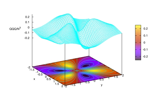
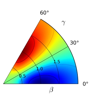
Figure 1: (Color online) Left: surface (grid) and contours (colored) representing $(\hat{Q}\times\hat{Q}\times\hat{Q})^{(0)}/N^{3}$ in the large $N$ limit with $\chi=0$ as a function of $\{x,y\}$. The coordinates on the plane are $x=\beta\cos\gamma$ and $y=\beta\sin\gamma$. Right: the same function in the fundamental $0^{\circ}\leq\gamma\leq 60^{\circ}$ wedge with contours (slightly different coloring scheme).

The upper left-part of the figure displays the value of the matrix element on the vertical coordinate, while the lower left-part is its projection on the plane with coordinates $x=\beta\cos\gamma$ and $y=\beta\sin\gamma$. The surface has prolate minima at $\beta=1$ and $\gamma=\frac{2\pi}{3}n$ and oblate maxima at $\beta=1$ and $\gamma=\frac{\pi}{3}(1+2n)$ with $n=0,1,2$. The contour map on the $x-y$ plane gives a color-coded projection of the surface values, with black/blue representing the (prolate) minimum and yellow/red representing the (oblate) maximum (see color bar on the right). For completeness sake we also give in the right-part of the figure a contour plot in the more standard $(\beta,\gamma)$ polar coordinates, limited to the $0^{\circ}\leq\gamma\leq 60^{\circ}$ wedge with a slightly different coloring scheme. Of course the character of the minima/maxima can be interchanged by an overall sign change. In conclusion, the cubic-Q term with $\chi=0$ only produces either prolate or oblate minima. Triaxiality or $\gamma-$unstability are not allowed with the $\hat{Q}\times\hat{Q}\times\hat{Q}$ term if $\chi=0$.

III The phase diagram in the large N limit

The study of the shape of a quantum system, in particular of atomic nuclei, proceeds through the study of the energy surface in the large $N$ limit. The shape is strictly defined in the thermodynamical limit. The procedure starts by calculating the potential energy surface in the large $N$ limit, then a minimization should be done, getting the equilibrium value of the deformation parameters.

III.1 Potential Energy Surface

The energy per boson in the large N limit can be readily calculated from Eq. (4):

$$E(\xi,k_{3},\chi,\beta,\gamma) = \xi\frac{\beta^{2}}{1+\beta^{2}}-(1-\xi)\Biggl{[}\frac{2}{7}~{}\frac{\beta^{2}}{(1+\beta^{2})^{2}}\Big{(}\chi^{2}\beta^{2}-2\sqrt{14}\chi\beta\cos 3\gamma+14\Big{)}$$ (10)

$$+ k_{3}~{}\frac{4}{49\sqrt{5}}~{}\frac{\beta^{3}}{(1+\beta^{2})^{3}}\Biggl{(}{\chi^{3}\beta^{3}(2\cos^{2}{3\gamma}-1)}-\sqrt{14}(3\chi^{2}\beta^{2}+14)\cos{3\gamma}+42\chi\beta\Biggr{)}\Biggr{]}.$$

Note that the $N$ dependence is eliminated due to the proper $N$ scaling of the different terms in the Hamiltonian and to the use of the energy per boson.

The presence of $\cos{3\gamma}$ and $\cos^{2}{3\gamma}$ in (10) can give rise to triaxiality. Let us start discussing the possibility of triaxiality for a simpler situation: an energy surface independent of $\beta$, but with the $\gamma$ dependence as in Eq. (10). In that case, one can write the energy surface as

$$E(\gamma)=a\cos^{2}{3\gamma}+b\cos{3\gamma}+c$$ (11)

where we take $a$, $b$, and $c$ as constants for the moment. This function admits triaxial extrema at

$$\gamma=(\pm\arccos{(-b/2a)}+2n\pi)/3$$ (12)

if $|-b/2a|\leq 1$, with $n=0,1,2$. When instead $\mid-b/2a\mid>1$, the extrema sit at $\gamma=2\pi n/3$ and $\gamma=(2n+1)\pi/3$, with $n=0,1,2$, and triaxiality is excluded.

In the general case, in which the coefficients $a$ and $b$ depend on $\beta$, as in the energy functional Eq. (10), the presence of terms depending on $\cos{3\gamma}$ and $\cos^{2}{3\gamma}$ can, in principle, produce triaxial shapes. It is clear that the existence of a triaxial minimum is linked to the inclusion of the cubic-Q term ($k_{3}\neq 0$) in the IBM Hamiltonian. The argument discussed above could, in principle, be valid even when the coefficients $a$ and $b$ depend on $\beta$, as long as their dependence on the equilibrium value of $\beta$, $\beta_{0}$, is smooth enough with respect to the control parameters of the Hamiltonian. However, for the cubic CQF Hamiltonian the latter argument is not so obvious, mainly due to the non continuous or very “fast” dependence of the $\beta$ equilibrium value in some intervals of the control parameters. To shed some light on this, one can calculate the value of $\mid-b/2a\mid$ (see Eq. (12)), which is the only necessary quantity to be known for getting the value of $\gamma$, and it can be written as

$$\left|-\frac{b}{2a}\right|=\left|-\frac{7\sqrt{70}\chi(1+\beta_{0}^{2})+\sqrt{14}k_{3}(14+3\chi^{2}\beta_{0}^{2})}{4k_{3}\chi^{3}\beta_{0}^{3}}\right|\;,$$ (13)

where $\beta_{0}$ is the equilibrium value of $\beta-$, that is, at the minimum of the energy. To rule out the possible existence of a triaxial region one has to prove as necessary and sufficient condition that $|\frac{-b}{2a}|>1$, for any value of the parameters in the Hamiltonian. In fact, this is true for $\xi=0$. Note that Eq. (13) does not depend explicitly on $\xi$, but its dependence comes in implicitly through the dependence of the equilibrium value of $\beta$ on $\xi$, $\chi$, and $k_{3}$.

To start with, we can easily calculate the value of $|\frac{-b}{2a}|$ in some limiting situations. In particular, $\lim_{\beta\to\infty}|\frac{-b}{2a}|=0$ or $\lim_{|\chi|\to\infty}|\frac{-b}{2a}|=0$ and therefore $\gamma=\pi/6$, but these situations are quite unrealistic. More interesting limiting situations are: $\lim_{\beta\to 0}|\frac{-b}{2a}|=\infty$, $\lim_{k_{3}\to\infty}|\frac{-b}{2a}|>16$ (this case is obtained considering that $\beta_{0}^{2}\chi^{2}$ is always larger than zero, remembering that $\beta_{0}$ in this equation is the value at the equilibrium point, taking into account that the larger is $|\chi|$, the larger is $\beta_{0}$ and, finally, fixing the maximum values for $|\chi|$ and $\beta_{0}$ to $\sqrt{7}/2$ and $1/\sqrt{2}$, respectively), $\lim_{k_{3}\to 0}|\frac{-b}{2a}|=\infty$, and $\lim_{\chi\to 0}|\frac{-b}{2a}|=\infty$. We will also prove later on that $|\frac{-b}{2a}|>1$ for $\xi=0$. On the other hand it is also true that the value of $\beta$ obtained for $\xi=0$ is always larger than the corresponding one for $\xi\neq 0$ (for the same values of $\chi$ and $k_{3}$). With these general ideas in mind, it is easy to see that $|\frac{-b}{2a}|>>1$ except, maybe, for a very narrow range of the parameters. Indeed, one can see that, once the values of the Hamiltonian parameters have been set, if we treat $\beta$ as a free parameter and not as a equilibirum value, one gets $|\frac{-b}{2a}|<1$ only in a very narrow range of $\beta$. In particular, it is possible to see, numerically, that this particular range of $\beta$ is placed in a region where $\beta$ exhibits a sudden drop. This is illustrated in Fig. 2, where the value of $|\frac{-b}{2a}|$ is plotted as a function of $\beta$, for $k_{3}=1$ and $\chi=-0.5$. It is clearly observed that only around $\beta\approx 0.934$ one gets $|\frac{-b}{2a}|<1$, but this particular value of $\beta$ falls in a rapidly changing region as it can be appreciated in the lower part of the figure, where the equilibrium value of $\beta$ is represented as a function of $\xi$.

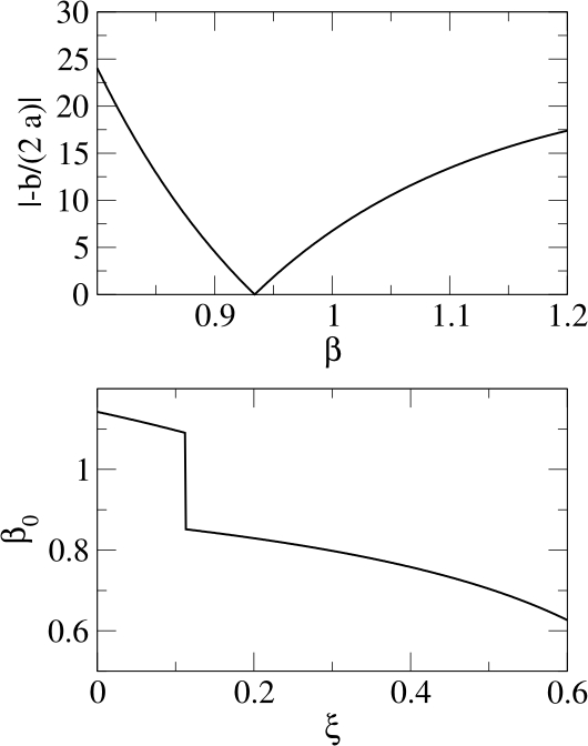
Figure 2: Upper part: value of $|\frac{-b}{2a}|$ (see text) as a function of $\beta$ for $k_{3}=1$ and $\chi=-0.5$. Equilibrium value of $\beta$ as a function of $\xi$.

As a conclusion of this qualitative discussion on possible triaxiality produced by the Hamiltonian (4), it can be said that one expects that the region supporting triaxial shapes is small, if any. We will quantify this idea in the following sections.

III.2 The coordinates

The pictorial representation of the phase space of the CCQH is an extension of the well-known Casten triangle (left plot in Fig. 3). In our case the parameter space becomes a tetrahedron, where the horizontal coordinates are related to the $\xi$ and $\chi$ control parameters in the Hamiltonian, while the vertical coordinate is directly connected to the coefficient of the $\hat{Q}\times\hat{Q}\times\hat{Q}$ term. We use the following parametrization:

$$\left\{\rho=1-\xi~{};~{}\phi=-\frac{\pi}{3}~{}\frac{\chi}{\sqrt{7}}~{};~{}z=\rho~{}k_{3}~{}\right\}.$$ (14)

In the studies presented below, the value of $\chi$ ranges from $-\sqrt{7}/2$ to $0$ and therefore the amplitude of the $\phi$ angle is $30^{\circ}$, $\rho$ ranges from $0$ to $1$ and $k_{3}$ is taken as positive. This range of control parameters allows to get the results for the full model space since the energy surface (10) presents the following prolate/oblate symmetry: $\chi\rightarrow-\chi$, $k_{3}\rightarrow-k_{3}$, $\gamma\rightarrow\pi/3-\gamma$. This allows to extend the results obtained in the case of $\chi<0$ and $k_{3}>0$ to the regions with $\chi>0$ and $k_{3}<0$.

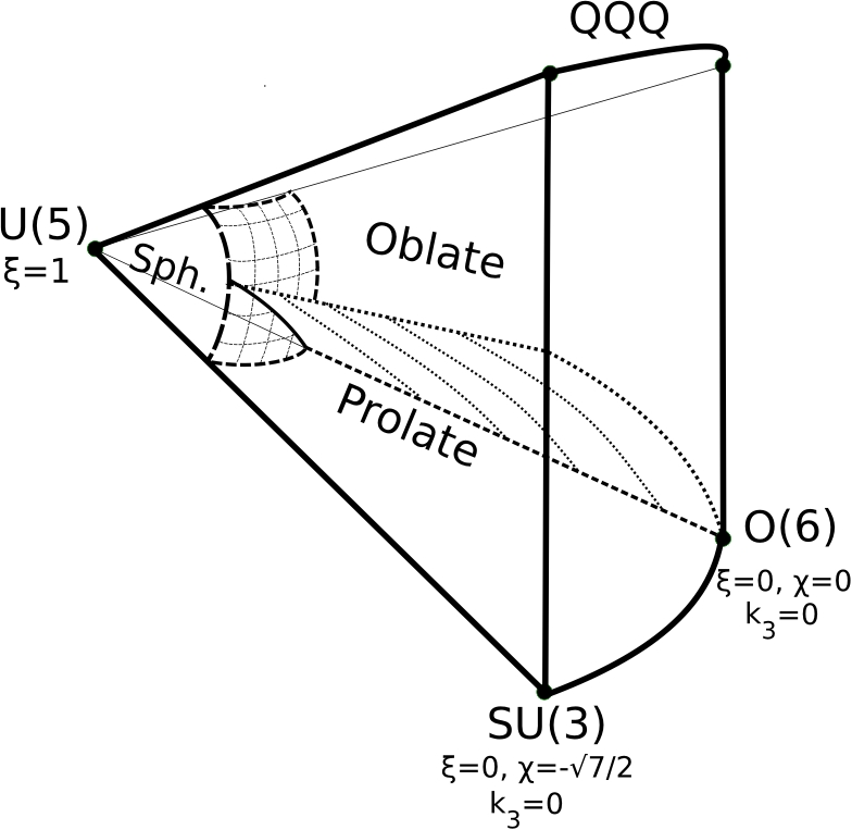
Figure 3: (Left) Schematic representation of the CCQH parameter space and coordinates. Four quadrants are present, of which only the first one is studied in detail as explained in the text. As a reference, the IBM dynamical symmetry limits are explicitly shown. (Right) Schematic phase diagram for the CCQH, corresponding to quadrant I in the figure on the left.

It is worth noting that due to the form of the Hamiltonian (4) it is not possible to reach a pure Cubic Q Hamiltonian, except for $k_{3}\to\infty$. However in Fig. 3 the upper part of the tetrahedron is labeled with $\hat{Q}\times\hat{Q}\times\hat{Q}$ to denote that this limit is reached for large values of $z=\rho k_{3}$. Anyway, in this study we will limit ourselves to moderated large values of $k_{3}$ (up to 10) since the cubic Q term is supposed to be a correction to the dominant QQ term.

First, the schematic phase diagram of the model Hamiltonian will be studied and then some particular relevant regions will be analyzed in more detail with the aim of singling out possible regions of triaxiality.

III.3 The geometry of the phase diagram

The resulting phase diagram for the Hamiltonian (4) is depicted in the right hand side of Fig. 3. Although a detailed explanation of the nature of this phase diagram will be given along this section, we already present the complete diagram here to facilitate the following analysis. The position of the critical surfaces are determined numerically, except for some particular regions of the phase diagram that can be obtained analytically. We have explored the parameter space to find out the position of the critical surfaces, following certain selected paths across the parameter space to clearly illustrate where the critical surfaces are placed and what is their character. This phase diagram is characterized by the existence of four different phases: spherical ($\rho\lesssim 0.2$, or $1>\xi\gtrsim 0.8$), prolate and oblate axially deformed shapes ($\rho\gtrsim 0.2$, or $\xi\lesssim 0.8$) and a very tiny region of triaxial shapes, occurring between the oblate/prolate separation surface close to the $\chi=\pm\sqrt{7}/2$ faces of the tetrahedron. Note that the existence of a spherical region is limited to moderate values of $k_{3}$. Due to the particular form of Hamiltonian (4), very lare values of $k_{3}$ will transform the spherical region almost in a single point around the origin. The two plotted surfaces correspond to first order phase transitions except along their intersection line, which is a second order phase transition line (full line in the right panel of Fig. 3). As we will explain in detail along this section, the prolate-oblate first order transition surface becomes a two-fold second order phase transitions surface for $\chi\approx-\sqrt{7}/2$, although these surfaces are extremely close and cannot be distinguished in Fig. 3.

The full phase space comprehend four tetrahedra (numbered I - IV) with a common U(5) vertex, shown in the left part of Fig. 3, while in the right part of the figure only the upper left quarter (I) with positive values of $k_{3}$ and negative values of $\chi$ is plotted. Apart from the spherical region close to $\xi=1$, that is always present, the upper right quadrant II ($k_{3}>0$ and $\chi>0$) contains only oblate shapes, while the opposite lower left quadrant III ($k_{3}<0$ and $\chi<0$) contains only prolate shapes. Finally, due to the prolate oblate/symmetry $\chi\rightarrow-\chi$, $k_{3}\rightarrow-k_{3}$, $\gamma\rightarrow\pi/3-\gamma$, the lower right quadrant IV can be obtained by rotating the first quadrant $180^{\circ}$ with respect to the $U(5)-O(6)$ axis. In order to illustrate how the phase diagram has been obtained we will show the results along several selected paths within quadrant I.

III.3.1 Paths from deformed to spherical shapes

First, we will explore the separation surface of spherical and deformed shapes. For that purpose, we start selecting $k_{3}=4$ and $\chi=-\sqrt{7}/2$ and we vary $\xi$. In Fig. 4 we observe a first order phase transition, where $\beta$ goes from a finite value to zero and $\gamma$ goes from $60^{\circ}$ (oblate shape) to undefined (spherical), when entering the spherical region. Note that the equilibrium value of $\beta$ for $\xi=0$ is $\beta=1/\sqrt{2}$. In the right part of the figure we have displayed the position of the path (green thick line) inside the phase diagram and also the position of the phase transition point (green circle). It should be noted that U(5) corresponds to $\xi=1$ and the surface SU(3)-O(6)-QQQ to $\xi=0$. In the following figures we include plots with similar interpretations. For $\chi=0$ one can obtain plots similar to Fig. 4, although in this case the transition occurs for a slightly larger value of $\xi$.

Figure 4: (Color online) Ground state energy and the equilibrium value of the shape variables $\beta$ and $\gamma$ as a function of $\xi$ along the path shown in the right part of the figure, for $k_{3}=4$ and $\chi=-\sqrt{7}/2$. Notice that the equilibrium value of $\gamma$ is undefined in the spherical region.

Now we consider a smaller value of $k_{3}$. We impose $k_{3}=1$ and $\chi=-\sqrt{7}/2$ and we vary the value of $\xi$. This trajectory is plotted in Fig. 5 and once more the existence of a first order phase transition can be noted, although it is not as abrupt as in the previous case. The value of $\gamma$ passes from zero (prolate shape) to undefined in the spherical region. Finally note that $\beta=\sqrt{2}$ for $\xi=0$.

Figure 5: (Color online) The same as in Fig. 4 but for $k_{3}=1$ and $\chi=-\sqrt{7}/2$.

Now, it is clear that there is a surface that separates spherical and deformed shapes at around $\xi=0.8$. In order to investigate the character of this surface, where the system changes from a spherical to a deformed shape, it is possible to carry out a Taylor expansion of the energy around the value $\beta=0$, obtaining:

$$E(\xi,k_{3},\chi,\beta,\gamma) = (-4+5\xi)\,\beta^{2}$$ (15)

$$- \frac{4}{35}(1-\xi)\left(2\sqrt{70}k_{3}+5\sqrt{14}\chi\right)\,\cos{3\gamma}\,\beta^{3}$$

$$+ \left(-\xi+(1-\xi)\left(8-\frac{24k_{3}\chi}{7\sqrt{5}}-\frac{2\chi^{2}}{7}\right)\right)\,\beta^{4}+\Theta(\beta^{5}).$$

This expression is very convenient because one can easily read off the order of the phase transition when crossing the surface. In general, the presence of a cubic term in $\beta$ implies that the system undergoes a first order phase transition Gilm81 , while its absence guaranties that the phase transition is of second order.

From equation (15) and the preceding discussion one notices that the spherical-deformed surface corresponds to a first order phase transition except when

$$k_{3}=-\frac{\sqrt{5}}{2}\chi,$$ (16)

which cancels the $\beta^{3}$ term and changes the transition type to second order. This second order phase transition line is the intersection of the spherical-deformed surface (studied here) and the prolate-oblate surface (to be studied in the next subsection). Therefore along this line spherical, prolate and oblate shapes coexist.

In order to show the characteristics of this second order phase transition line we have followed a path that crosses the spherical-deformed surface precisely through this line. This is illustrated in Fig. 6, where a second order phase transition appears at $\xi=4/5$.

Figure 6: (Color online) The same as in Fig. 4 or 5 but for $k_{3}=1$ and $\chi=-2/\sqrt{5}$ (second order phase transition).

No discontinuity is observed neither in the order parameter $\beta$, nor in the energy or in its first derivative (not shown in the figure). The discontinuity appears in the second derivative of the energy confirming that the line (16) is of the second order type.

With respect to the existence or not of triaxiality in the region close to spherical shapes, in expression (15) only the $\cos{3\gamma}$ shows up, but the $\cos^{2}{3\gamma}$ dependence will appear together with $\beta^{6}$ terms and therefore it will generate a value $|\frac{-b}{2a}|>>1$ since the coefficient of $\cos{3\gamma}$ (a) is much smaller than the one of $\cos^{2}{3\gamma}$ (b) for $\beta<1$. Therefore, there is no possibility of triaxiality close to the spherical region.

Finally, note that for every value of $\xi$, with the exception of $\xi=1$, it always exists a value of $k_{3}$ that marks the appearance of an additional deformed minimum. This situation is quite different with respect to the one obtained with two body Hamiltonians, where a value of $\xi\gtrsim 0.8$ implies a spherical minimum regardless of the value of $\chi$. In the phase diagram depicted in the right part of Fig. 3 this fact cannot be noticed because of the moderated values of $k_{3}$ used along the diagram.

III.3.2 Paths from deformed prolate to deformed oblate shapes

Figure 7: (Color online) Ground state energy, equilibrium shape variables $\beta$ and $\gamma$ as a function of $k_{3}$ for $\xi=0$ and $\chi=-\sqrt{7}/2$.

Now, we explore the separation surface between prolate and oblate shapes, starting from the $\xi=0$ surface and then generalizing to $\xi\neq 0$.

The $\xi=0$ case: interplay of $\hat{Q}\cdot\hat{Q}$ and $(\hat{Q}\times\hat{Q}\times\hat{Q})^{(0)}$

In this subsection the $\xi=0$ ($\rho=1$) surface (SU(3)-O(6)-QQQ) is studied. For pedagogical reasons we start our study by setting $\chi=-\sqrt{7}/2$ (the vertical line between SU(3) and QQQ in Fig. 3) and later on we will generalize the outcome to arbitrary values of $\chi$. For the case, $\xi=0,\chi=-\sqrt{7}/2$, the extrema of the $-\hat{Q}\cdot\hat{Q}/N^{2}$ term in the large N limit are listed in Table 1. In this Table the signs of the second derivative of the energy with respect to both shape parameters, $\beta$ and $\gamma$, and the character of the extrema (M for maximum, m for minimum and s.p. for saddle point) are given. To avoid equivalent shapes related with the symmetries of the P.E.S.

we impose the constraints $\beta\geq 0$ and $0\leq\gamma\leq\pi/3$. Summarizing the information in Table 1, the surface obtained from the $-\hat{Q}\cdot\hat{Q}/N^{2}$ term presents: a spherical maximum with no dependence on $\gamma$, a prolate minimum for $\beta=\sqrt{2}$, a saddle point in the oblate side for $\beta=1/\sqrt{2}$ and an oblate maximum for $\beta=2\sqrt{2}$. Note that at the extrema there are no off-diagonal terms in the Hessian matrix.

$~{}~{}~{}~{}\beta~{}~{}~{}~{}$	$~{}~{}~{}~{}\gamma~{}~{}~{}~{}$	$\partial^{2}E/\partial\beta^{2}$	$\partial^{2}E/\partial\gamma^{2}$	character
0	$-$	$0$	$-$	M
$1/\sqrt{2}$	$\pi/3$	$+$	$-$	sp
$\sqrt{2}$	$0$	$+$	$+$	m
$2\sqrt{2}$	$\pi/3$	$-$	$-$	M

Table 1: Extrema of $-\hat{Q}\cdot\hat{Q}/N^{2}$, for $\chi=-\sqrt{7}/2$, along with their character. The sign of the second derivatives with respect to $\beta$ and $\gamma$ are also given (see text).

A similar study can be done for $-(\hat{Q}\times\hat{Q}\times\hat{Q})^{(0)}/N^{3}$. The characters of the extrema for the surface produced by this term are listed in Table 2. In this case there are a spherical maximum, an oblate minimum at $\beta=1/\sqrt{2}$, a prolate maximum at $\beta=\sqrt{2}$ and, finally, an oblate saddle point at $\beta=2\sqrt{2}$. Moreover there is also a minimum for $\beta\to\infty$ and $\gamma=\pi/6$. Note that, again, at the extrema there are no off-diagonal terms in the Hessian matrix. It is worth noting that the extrema for both, $-\hat{Q}\cdot\hat{Q}/N^{2}$ and $-(\hat{Q}\times\hat{Q}\times\hat{Q})^{(0)}/N^{3}$ coincide, although their character, either minimum or maximum, can be different.

$~{}~{}~{}~{}\beta~{}~{}~{}~{}$	$~{}~{}~{}~{}\gamma~{}~{}~{}~{}$	$\partial^{2}E/\partial\beta^{2}$	$\partial^{2}E/\partial\gamma^{2}$	character
0	$-$	$0$	$-$	sp
$1/\sqrt{2}$	$\pi/3$	$+$	$+$	m
$\sqrt{2}$	$0$	$-$	$-$	M
$2\sqrt{2}$	$\pi/3$	$0$	$0$	s.p.

Table 2: Same as Table 1 but for $-(\hat{Q}\times\hat{Q}\times\hat{Q})^{(0)}/N^{3}$.

A Hamiltonian built upon a linear combination of $-\hat{Q}\cdot\hat{Q}$ and $-(\hat{Q}\times\hat{Q}\times\hat{Q})^{(0)}$ is expected to possess eigenstates with large quadrupole moments and small fluctuations around their equilibrium values. This kind of state is eigenstate of the quadrupole operator, as well as of both, $\hat{Q}\cdot\hat{Q}$ and $(\hat{Q}\times\hat{Q}\times\hat{Q})^{(0)}$ GK ; Jolo04 . This is the reason why the extrema points of both parts of the Hamiltonian under study coincide Jolo04 .

In general, a linear combination of $-\hat{Q}\cdot\hat{Q}$ and $-(\hat{Q}\times\hat{Q}\times\hat{Q})^{(0)}$ always generates a spherical maximum for $\beta=0$, an oblate maximum or saddle point at $\beta=2\sqrt{2}$ and a competition between two minima, one prolate at $\beta=\sqrt{2}$ and the other one oblate at $\beta=1/\sqrt{2}$. The above situation corresponds to a first order phase transition and it excludes the presence of a triaxial minimum.

Fig. 7 gives the evolution of the ground state energy and the equilibrium value of $\beta$ and $\gamma$ for the path along the line $\chi=-\sqrt{7}/2$ and $\xi=0$. This figure shows the typical ingredients of a first order phase transition. There is a discontinuity in the first derivative of the energy and a discontinuity in the value of $\beta$ and $\gamma$. For low values of $k_{3}$ the minimum corresponds to $\beta=\sqrt{2}$ and $\gamma=0^{\circ}$, while for large values to $\beta=1/\sqrt{2}$ and $\gamma=60^{\circ}$. The critical value of the control parameter corresponds to $k_{3}=\sqrt{35}/{3}$. This figure is similar to Fig. 2 appearing in Ref. Aria04 although there the phase transition is second order and $\gamma$ goes from $0^{\circ}$ to $60^{\circ}$ in a smooth way and therefore a broad region of triaxiality exists.

An interesting case happens for $k_{3}=\frac{\sqrt{35}}{3}$, for which the prolate minimum ($\beta=\sqrt{2}$) flattens (becoming a maximum for larger values), i.e. $\partial^{2}E/\partial\beta^{2}=\partial^{2}E/\partial\gamma^{2}=0$. Additionally, the flat prolate and the oblate minima become degenerate with energy $E=-\frac{2}{3}$, being also degenerate with the minimum at $\beta\rightarrow\infty$, $\gamma=\pi/6$. This is illustrated in Fig. 8.

Figure 8: (Color online) Energy surface for $-\hat{Q}\cdot\hat{Q}/N^{2}-\frac{\sqrt{35}}{3}(\hat{Q}\times\hat{Q}\times\hat{Q})^{(0)}/N^{3}$ with $\chi=-\sqrt{7}/2$, corresponding to the green dot of the right part of the figure. Note the existence of a prolate and an oblate degenerated minima.

For $k_{3}<\frac{\sqrt{35}}{3}$ the only minimum is the prolate one, that becomes flat for $k_{3}=\frac{\sqrt{35}}{3}$. For $k_{3}>\frac{\sqrt{35}}{3}$, the only minimum is the oblate one. Therefore, at $k_{3}=\frac{\sqrt{35}}{3}$ the spinodal and the antispinodal points coincide and also are degenerate (first order phase transition point).

It is possible to extend the preceding study to a generic value of $\chi$. Without loss of generality, we choose $\chi<0$. In this case the position of the possible minima are given in Table 3.

$\beta$	$\gamma$
$\displaystyle{\frac{\chi}{\sqrt{14}}+\frac{\sqrt{14+\chi^{2}}}{\sqrt{14}}}$	$\pi/3$
$\displaystyle{-\frac{\chi}{\sqrt{14}}+\frac{\sqrt{14+\chi^{2}}}{\sqrt{14}}}$	0

Table 3: Position of the possible minima for a linear combination $-\hat{Q}\cdot\hat{Q}/N^{2}-k_{3}(\hat{Q}\times\hat{Q}\times\hat{Q})^{(0)}/N^{3}$, with a generic value of $\chi<0$.

Again there is a competition between the prolate minimum, coming from the $-\hat{Q}\cdot\hat{Q}/N^{2}$ term an the oblate one, generated with the $-(\hat{Q}\times\hat{Q}\times\hat{Q})^{(0)}/N^{3}$ term. In this case there exists a coexistence region, but again there is no room for triaxiality. In particular, the position of spinodal ($\gamma=\pi/3$) and antispinodal ($\gamma=0$) points are given by

$$k_{3}\left(\left.\partial^{2}E/\partial\gamma^{2}\right|_{\gamma=\left\{{\pi/3\atop 0}\right\}}=0\right)=-\frac{49\sqrt{5}\chi\left(\chi^{2}\pm\chi\sqrt{\chi^{2}+14}+14\right)}{4\chi^{6}\pm 4\chi^{5}\sqrt{\chi^{2}+14}+63\chi^{4}\pm 35\chi^{3}\sqrt{\chi^{2}+14}+147\chi^{2}+686},$$ (17)

the upper (lower) sign corresponds to $\gamma=\pi/3$ (0). The value of $k_{3}$ where the two minima become degenerate (critical line) reads

$$k_{3c}=-\frac{7\sqrt{5}\chi}{2\chi^{2}+7}.$$ (18)

In Fig. 9 the spinodal, the antispinodal and the critical values of $k_{3}$ are represented in the $(k_{3},\chi)$ plane for $\xi=0$. This figure clearly shows the existence of a coexistence region and the absence of a triaxial region in the $\xi=0$ surface.

Additional extrema to the ones given in the above mentioned table can appear which do not correspond to minima.

Figure 9: (Color online) Value of the spinodal ($\gamma=\pi/3$), antispinodal ($\gamma=0$) and critical value lines of $k_{3}$ as a function of $\chi$ for $\xi=0$.

The $\xi\neq 0$ case: The prolate-oblate-triaxial critical surface

The analytical arguments used in the preceding discussion are no longer valid when the $U(5)$ term gives a contribution to the energy surface, i.e. $\xi\neq 0$, however they suggest that the parameter space region that gives rise to a triaxial minimum should be rather small. It is not possible to obtain analytically the expression of the equilibrium value of $\gamma$ for a general energy surface.

To study numerically the deformed region for this particular Hamiltonian we calculate the value of the energy, $\beta$ and $\gamma$ along some particular lines that go through the phase diagram and cross the prolate-oblate separation surface. In Fig. 10 we select a particular path with $\xi=0.5$ and $\chi=-1$ with $k_{3}$ ranging from $0$ to $4$. In this figure the presence of a first order phase transition shows up because there exists a clear discontinuity in the values of $\beta$ and $\gamma$, when crossing the prolate-oblate surface. Therefore there is a jump from the prolate to the oblate minimum at the point where they become degenerate and the triaxiality is forbidden. The same happens for other values of $\xi$ and $\chi$.

However a more detailed inspection shows that there exists a very tiny region of triaxiality around $\chi\approx-\sqrt{7}/2$, for $\xi<4/5$. This is clearly illustrated in Fig. 11, where the lines that separate the prolate, oblate and triaxial regions are plotted for a value of $\xi=0.5$. Note that the triaxial region occurs for $\chi$ close to the limiting value of $-\sqrt{7}/2$. At this limit $k_{3}\in[1.752-1.791]$. The lower part of the figure corresponds to prolate minima, while the upper part to oblate minima. The box on the vertical left side shows the blowup of this region: there is indeed a small range of values where it is possible to find triaxial minima by numerical procedure. The more one moves away from the value $\chi=-\frac{\sqrt{7}}{2}$, the narrower this range becomes, due to the delicate interplay between the quadratic and cubic terms.

Figure 10: (Color online) Ground state energy and equilibrium value of the shape variables $\beta$ and $\gamma$ as a function of $k_{3}$, for $\xi=0.5$ and $\chi=-1$ for the path shown on the right.

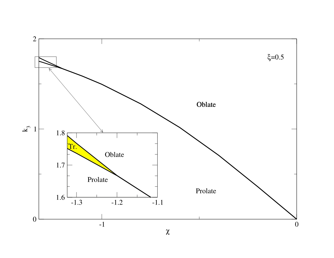
Figure 11: (Color online) Section of the three-dimensional parameter space with $\xi=0.5$ and $N\rightarrow\infty$. The yellow inset shows the tiny triaxial region (see text) that is found at $\chi\approx-\sqrt{7}/2$.

We can see in a clearer way the onset of a triaxial minimum in Fig. 12. Here we have plotted several potential energy surfaces corresponding to points along the left vertical axis of Fig. 11 with $\chi=-\frac{\sqrt{7}}{2}$ and $\xi=0.5$. The minimum is clearly prolate for small values of $k_{3}$ and it starts to widen as one approaches the region $k_{3}\sim 1.7$. From approximately $1.752$ to $1.791$ the minimum is triaxial, but very shallow and therefore invisible at the present scale of $(\beta,\gamma)$. We show in Fig. 13, for completeness sake, the close up of the minimum for $k_{3}=1.77$. Increasing again the value of $k_{3}$ leads to an axially deformed oblate minimum. It is worth noting that the change through the triaxial region is extremely swift and some care must be taken in the minimization. One can appreciate the extremely shallow character of the triaxial minimum that extends from the axially prolate till the oblate minimum, very much in a similar way to Fig. 8 where prolate and oblate minima are degenerate and no triaxial minimum exists.

$k_{3}=0.0$	$k_{3}=1.5$	$k_{3}=1.77$	$k_{3}=2.0$	$k_{3}=3.0$

Figure 12: (Color online) Potential energy surfaces for the CCQH for $\chi=-\sqrt{7}/2$ and $\xi=0.5$, with different values of $k_{3}$ indicated in the figure. The observed minima range from an axially deformed prolate minimum for $k_{3}=0.0$ and $k_{3}=1.5$ to an oblate one for $k_{3}=2.0$ and $k_{3}=3.0$ , passing through the triaxial region. The triaxial minimum when $k_{3}=1.77$ is not apparent from this figure, because it is very shallow (see next figure).

The existence of the triaxial region is confirmed by inspecting contour plots of the potential energy surface along a suitable trajectory of the parameter space, rather than just looking at the plots of $\beta$ and $\gamma$ as a function of the parameters $\xi$, $\chi$ and $k_{3}$.

Figure 13: (Color online) Closeup of the potential energy surface of Eq. (10) with $\chi=-\sqrt{7}/2$, $\xi=0.5$ and $k_{3}=1.77$, clearly showing a shallow triaxial minimum at $\beta\sim 0.62$ and $\gamma\sim 23.4^{\circ}$. One can prove, with similar plots, that the prolate minimum smoothly shifts through the triaxial region and finally becomes oblate.

Finally we present in Fig. 14 a cut of the triaxial region as a function of $\xi$ and $k_{3}$ for a constant value of $\chi=-\sqrt{7}/2$. A very small triaxial region is always found, except for $\xi=0$, between the lower prolate region and the upper oblate one (see inset of Fig. 14) and terminates in correspondence with the spherical phase that occurs for high values of $\xi$. In a preceding subsection we have discussed that the point connecting with the spherical phase is indeed a single point as well as the one at $\xi=0$.

Figure 14: (Color online) Section of the three-dimensional parameter space with $\chi=-\frac{\sqrt{7}}{2}$ as a function of $\xi$ and $k_{3}$. The inset shows the triaxial region in yellow on a finer vertical scale (see text).

A final question should be answered: what is the order of the phase transition developed in crossing the prolate-triaxial-oblate surface? In the region of triaxiality the surface evolves into two different sheets where second order phase transitions exist. As far as we move from $\chi=-\sqrt{7}/2$ this two-fold surface collapses in a single one and the phase transition becomes of the first order.

Since the small triaxial region appears in the deformed area close to $\chi=-\sqrt{7}/2$, we present in Fig. 15 a path with fixed $\chi=-\sqrt{7}/2$ and $\xi=0.5$ and changing $k_{3}$. Once more we plot in this figure the evolution of the ground state energy and the equilibrium value of $\beta$ and $\gamma$. Again low values of $k_{3}$ give rise to prolate shapes, while the larger ones produce oblate forms, but a narrow region of triaxiality exists around $k_{3}\sim 1.75-1.79$. The scale does not allow to discriminate, therefore we have enlarged it in the inset that shows two, very close, second order phase transitions.

Figure 15: (Color online) Ground state energy, shape variables $\beta$ and $\gamma$ as a function of $k_{3}$ for $\xi=0.5$ and $\chi=-\sqrt{7}/2$ for the path shown on the right.

One from prolate to triaxial at around $k_{3}=1.75$ and a second one from triaxial to oblate at around $k_{3}=1.79$. As soon as we depart from the $\chi=-\sqrt{7}/2$ surface these two second order surfaces approach more and more up to a point in which both coincide and apparently transform into a first order surface that directly separates prolate and oblate shapes, without any triaxiality in between. It is very difficult numerically to determine whether the triaxial region narrows indefinitely or rather ends up in a tricritical point.

III.3.3 A path going from spherical through oblate and prolate shapes

As a final calculation we study a trajectory that crosses the spherical-deformed surface as well as the prolate-oblate one. The appropriate values of $k_{3}$ and $\chi$ are constrained by equations (16) and (18) and should verify

$$-\frac{7\sqrt{5}\chi}{2\chi^{2}+7}>k_{3}>-\frac{\sqrt{5}}{2}\chi.$$ (19)

We choose $k_{3}=1.5$ and $\chi=-2/\sqrt{5}$, which fulfil (19), and vary the value of $\xi$. This path is depicted in Fig. 16 and two first order phase transitions are clearly marked. From left to right, the first one has a discontinuity in $\beta$ between two finite values changing at the same time $\gamma$ from $0^{\circ}$ to $60^{\circ}$. In the second one the system goes from the oblate phase to the spherical one, changing $\beta$ from a finite to a zero value and $\gamma$ from $60^{\circ}$ to undefined.

Figure 16: (Color online) The same as in Fig. 4 but for $k_{3}=1.5$ and $\chi=-2/\sqrt{5}$.

IV Some applications

IV.1 Spherical to axially deformed critical point: X(5)

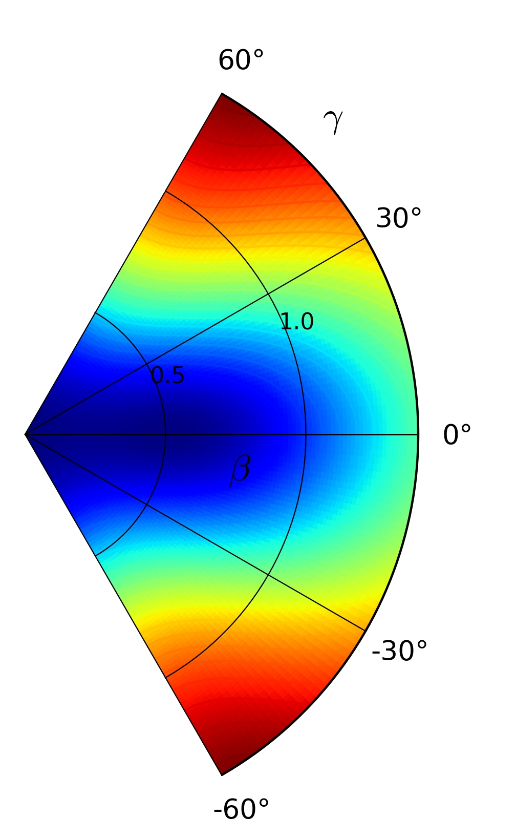
Figure 17: (Color online) Potential energy surface (left) obtained from (4) with $\chi=0,\xi=0.9$ and $k_{3}=-9.5$. The valley along the $\gamma=0^{\circ}$ direction for prolate deformations resembles the potential used in the X(5) solution of the Bohr Hamiltonian Iac2 .Right hand side: two sections of the energy surface around the equilibrium value of the deformation parameters have been plotted as a function of $\beta$ and $\gamma$, respectively.

An interesting special case is to keep $\chi=0$, in order to eliminate the driving effect of the $\hat{Q}\cdot\hat{Q}$ term toward axial deformation. In the left part of Fig. 17 a large value of $k_{3}$ generates a surface with an almost flat valley along the $\beta$ direction, while the prolate (oblate) confinement in $\gamma$ is due to the negative (positive) sign in front of the $(\hat{Q}\times\hat{Q}\times\hat{Q})^{(0)}$ term. This case has a potential energy surface that has a flat shape qualitatively similar to the $V(\beta,\gamma)$ potential used in the X(5) critical point symmetry Iac2 , with due differences: it is generated through a set of parameters $\chi=0$, $\xi=0.9$, and $k_{3}=-9.5$ (a positive value would generate an equivalent oblate shape), the potential does not tend to infinity, but goes smoothly to an asymptotic value and the periodicity in $\gamma$ is retained, at a variance with a harmonic oscillator. The bottom of the potential is not exactly flat, nor the behavior approximates a $\beta^{4}$ dependence, but the fact that a potential energy surface that mimics X(5) could be obtained with $\chi=0$ is somewhat surprising, because it has been used to associate X(5) to a case that is intermediate between spherical and axially prolate shapes, while here we do not even need to set $\chi=-\sqrt{7}/2$.

IV.2 Application to a schematic Hamiltonian

As an application, we can now use the formula for the matrix element of the $(\hat{Q}\times\hat{Q}\times\hat{Q})^{(0)}$ operator with $\chi~{}=~{}0$ within the boson coherent state formalism to give further insight into the results obtained by Rowe and Thiamova for the schematic Hamiltonian (3) RoTi ; Thi . The parameter $k$ is allowed to vary from zero to large positive values. In Fig. 18 we have plotted several contour maps corresponding to $k=0.0,~{}0.58776,~{}1.0$, and $10.0$. Notice that the $\Lambda$ term alone ($k=0$) just gives a spherical minimum, because its matrix element in the coherent state approach is just proportional to $\beta^{2}$.

k=0.0	k$\sim$0.58776	k=1.0	k=10.0

Figure 18: (Color online) Potential energy surfaces for the Hamiltonian (3) with $N=10$ and different values of $k:0.0,k_{cr},1.0$ and $k=10.$. The minimum (blue) ranges from spherical to axially deformed prolate. Vertical scales change along the transition.

From the figure one can appreciate how, with growing value of $k$, the minimum moves from the spherical configuration to the axially deformed prolate one. This is due to the competition between the spherically driving term $\Lambda$ and the cubic interaction term $(\hat{Q}\times\hat{Q}\times\hat{Q})^{(0)}$ that has a stable axial minimum, despite having $\chi=0$. We have collected in Fig. 19 several cuts of the potential energy surface along $\gamma=0^{\circ}$, for the values $k=0.0,~{}0.2,~{}0.4,~{}k_{cr},~{}0.8$, and $1.0$. Alongside the ever-present minimum at $\beta=0$, this potential admits a second deformed local minimum, that starts to appear after $k\sim 0.51$. The critical point for the first order phase transition is found around $k_{cr}\sim 0.58776$, where two minima are degenerate. After this point the deformed minimum prevails. The values discussed above are valid with the particular choice of $N=10$ and with the Hamiltonian as given originally in (3). Although it is immaterial to the present discussion, one should notice that, while the O(5) scalar term is linear with the boson number, the $(\hat{Q}\times\hat{Q}\times\hat{Q})^{(0)}$ term is cubic with $N$ and therefore one should better choose a Hamiltonian that is properly normalized to get rid of the different scaling with the boson number.

Figure 19: (Color online) Cuts along $\gamma=0^{\circ}$ of the potential energy surfaces for the Hamiltonian (3) with $\chi=0$ and $N=10$ for several values of $k$ from $0.0$ to $1.0$. At the value $k_{cr}\sim 0.58776$ it shows the typical signs of a first order phase transition. Purple dots indicate the position of minima.

Notice that Ref. piet uses a slightly different Hamiltonian having $\hat{L}\cdot\hat{L}$ as a spherical term: although it is most certainly important to use the proper terms when calculating an IBM spectrum, it is less critical here, since both these operators have matrix elements proportional to $\beta^{2}$ (albeit not with the same coefficients). In both cases piet ; RoTi triaxial minima are clearly not possible. Moreover, the inclusion of the cubic term, even with $\chi=0$, forbids the existence of a $\gamma-$independent solution.

V Conclusions

We have calculated the potential energy surface of the cubic $(\hat{Q}\times\hat{Q}\times\hat{Q})^{(0)}$ term within the coherent state formalism with the most general expression for the quadrupole operator. This has allowed us to confirm the results of Ref. piet ; RoTi concerning the fact that this term with $\chi=0$ can generate axially deformed minima, but in addition it has been shown that the cubic term has already a dependence on $\cos^{2}{3\gamma}$ (for $\chi\neq 0$) together with the dependence on $\cos{3\gamma}$ (obtainable also when $\chi=0$). Therefore a Hamiltonian containing this term may generate triaxiality without the need to resort to the more complicated $(\hat{Q}\times\hat{Q}\times\hat{Q})^{(0)}\cdot(\hat{Q}\times\hat{Q}\times\hat{Q})^{(0)}$ expression of Ref. Thi .

After a discussion of its general features, we have used it to extend the Consistent-Q Hamiltonian to the Cubic Consistent-Q Hamiltonian, of which we have discussed the phase space, discovering that a triaxial region can indeed be found, between the oblate and prolate phases. This region is extremely tiny (at least in the particular parameterization chosen, if compared to the other phases), and can be pinpointed numerically only very close to the limiting values of $\chi\sim\pm\sqrt{7}/2$. The inspection of the PES confirmed that the minimum is indeed triaxial inside this region. It is not clear, at the moment, if the prolate and oblate phases are always separated by a region of triaxiality that progressively tails off as one goes to $\chi=0$ or if the triaxial region disappear at some point. The numerical results suggest that this tiny triaxial region finishes in a line where prolate, oblate and triaxial shapes coexist, i.e. a tricritical line.

References

- (1) A. Bohr and B. Mottelson, Nuclear Structure, Benjamin, Reading, Massachusetts (1975).
- (2) F. Iachello and A. Arima, The Interacting Boson Model, Cambridge Univ. Press (1987).
- (3) J.N. Ginocchio and M.W. Kirson, Nucl. Phys. A 350, 31 (1980).
- (4) D.D. Warner and R.F. Casten, Phys. Rev. C 28, 1798 (1983).
- (5) P. Van Isacker, A. Bouldjedri, and S. Zerguine, Nucl. Phys. A 836, 225 (2010).
- (6) K. Heyde, P. van Isacker, M. Waroquier and J. Moreau, Phys. Rev. C 29, 1420 (1984).
- (7) J.E. García-Ramos, Ph.D. Thesis, University of Sevilla (Spain) (1999), unpublished.
- (8) J.E. García-Ramos, C.E. Alonso, J.M. Arias, and P. Van Isacker, Phys. Rev. C 61, 047305 (2000).
- (9) J.E. García-Ramos, J.M. Arias, and P. Van Isacker, Phys. Rev. C 62, 064309 (2000).
- (10) Various Authors, Contemporary Concepts in Physics, vol.6, entitled Algebraic Approaches to Nuclear Structure, Ed. R.Casten, Harwood Academic Publishers, Chur, Switzerland (1993)
- (11) D. Bonatsos, Interacting Boson Models of Nuclear Structure, Oxford Science Publications (1988)
- (12) R.V. Jolos, Phys. Part. Nucl. 35, 225 (2004).
- (13) P. Van Isacker, Phys. Rev. Lett. 83, 4269 (1999).
- (14) D.J. Rowe and G. Thiamova, Nucl. Phys. A 760, 59 (2005).
- (15) G. Thiamova, Eur. Phys. J. A 45, 81 (2010).
- (16) L. Fortunato, unpublished.
- (17) P. Van Isacker and J.Q. Chen, Phys. Rev. C 24, 684 (1981).
- (18) S. Dusuel, J. Vidal, J.M. Arias, J. Dukelsky, J.E. García-Ramos, Phys. Rev. C 72, 011301R (2005).
- (19) S. Dusuel, J. Vidal, J.M. Arias, J. Dukelsky, J.E. García-Ramos, Phys. Rev. C 72, 064332 (2005).
- (20) R. Gilmore, Catastrophe theory for scientists and engineers, Wiley, New York (1981).
- (21) J.M. Arias, J. Dukelsky, and J.E. García-Ramos, Phys. Rev. Lett. 93, 212501 (2004).
- (22) F. Iachello, Phys. Rev. Lett. 87, 052502 (2001).