Bessel process, Schramm-Loewner evolution, and Dyson model
– Complex Analysis applied to
Stochastic Processes and Statistical Mechanics –

Abstract

Bessel process is defined as the radial part of the Brownian motion (BM) in the $D$-dimensional space, and is considered as a one-parameter family of one-dimensional diffusion processes indexed by $D$, BES^(D). First we give a brief review of BES^(D), in which $D$ is extended to be a continuous positive parameter. It is well-known that $D_{\rm c}=2$ is the critical dimension such that, when $D\geq D_{\rm c}$ (resp. $D<D_{\rm c}$), the process is transient (resp. recurrent). Bessel flow is a notion such that we regard BES^(D) with a fixed $D$ as a one-parameter family of initial value $x>0$. There is another critical dimension $\overline{D}_{\rm c}=3/2$ and, in the intermediate values of $D$, $\overline{D}_{\rm c}<D<D_{\rm c}$, behavior of Bessel flow is highly nontrivial. The dimension $D=3$ is special, since in addition to the aspect that BES⁽³⁾ is a radial part of the three-dimensional BM, it has another aspect as a conditional BM to stay positive.

Two topics in probability theory and statistical mechanics, the Schramm-Loewner evolution (SLE) and the Dyson model (i.e., Dyson’s BM model with parameter $\beta=2$), are discussed. The SLE^(D) is introduced as a ‘complexification’ of Bessel flow on the upper-half complex-plane, which is indexed by $D>1$. It is explained that the existence of two critical dimensions $D_{\rm c}$ and $\overline{D}_{\rm c}$ for BES^(D) makes SLE^(D) have three phases; when $D\geq D_{\rm c}$ the SLE^(D) path is simple, when $\overline{D}_{\rm c}<D<D_{\rm c}$ it is self-intersecting but not dense, and when $1<D\leq\overline{D}_{\rm c}$ it is space-filling. The Dyson model is introduced as a multivariate extension of BES⁽³⁾. By ‘inheritance’ from BES⁽³⁾, the Dyson model has two aspects; (i) as an eigenvalue process of a Hermitian-matrix-valued BM, and (ii) as a system of BMs conditioned never to collide with each other, which we simply call the noncolliding BM. The noncolliding BM is constructed as a harmonic transform of absorbing BM in the Weyl chamber of type A, and as a complexification of this construction, the complex BM representation is proposed for the Dyson model. Determinantal expressions for spatio-temporal correlation functions with the asymmetric correlation kernel of Eynard-Mehta type are direct consequence of this representation. In summary, ‘parenthood’ of BES^(D) and SLE^(D), and that of BES⁽³⁾ and the Dyson model are clarified.

Other related topics concerning extreme value distributions of noncolliding diffusion processes, statistics of characteristic polynomials of random matrices, and scaling limit of Fomin’s determinant for loop-erased random walks are also given.

We note that the name of Bessel process is due to the special function called the modified Bessel function, SLE is a stochastic time-evolution of complex analytic function (conformal transformation), and the Weierstrass canonical product representation of entire functions plays an important role for the Dyson model. Complex analysis is effectively applied to study stochastic processes of interacting particles and statistical mechanics models exhibiting critical phenomena and fractal structures in equilibrium and nonequilibrium states.
Keywords   Complexification, Multivariate extension, Conformal transformation, Random matrices, Entire functions

1 Family of Bessel processes

1.1 One-dimensional and $D$-dimensional Brownian motions

We consider motion of a Brownian particle in one dimensional space $\mathbb{R}$ starting from $x\in\mathbb{R}$ at time $t=0$. At each time $t>0$ particle position is randomly distributed, and each realization of path is labeled by a parameter $\omega$. Let $\Omega$ be the sample path space and $B^{x}(t,\omega)$ denote the position of the Brownian particle at time $t>0$, whose path is realized as $\omega\in\Omega$. Let $(\Omega,{\cal F},{\rm P})$ be a probability space. The one-dimensional standard Brownian motion (BM), $\{B^{x}(t,\omega)\}_{t\in[0,\infty)},x\in\mathbb{R}$, has the following three properties.

1.  $B^{x}(0,w)=x$ with probability one (abbr. w.p.1).

2.  For any fixed $\omega\in\Omega$, $B^{x}(t,\omega)$ is a real continuous function of $t$. In other words, $B^{x}(t)$ has a continuous path.

3.  For any sequence of times, $t_{0}\equiv 0<t_{1}<\cdots<t_{M},M\in\mathbb{N}\equiv\{1,2,3,\dots\}$, the increments $\{B^{x}(t_{i})-B^{x}(t_{i-1})\}_{i=1}^{M}$ are independent, and distribution of each increment is normal with mean $m=0$ and variance $\sigma^{2}=t_{i}-t_{i-1}$. It means that for any $1\leq i\leq M$ and $\ell<r$,

$${\rm P}(B^{x}(t_{i})-B^{x}(t_{i-1})\in[\ell,r])=\int_{\ell}^{r}p_{t_{i}-t_{i-1}}(\delta|0)d\delta,$$

where we define for $a,b\in\mathbb{R}$

$$p_{t}(b|a)=\left\{\begin{array}[]{ll}\displaystyle{\frac{1}{\sqrt{2\pi t}}e^{-(a-b)^{2}/2t}},&\quad\mbox{for $t>0$},\cr\delta(a-b),&\quad\mbox{for $t=0$}.\end{array}\right.$$ (1.1)

If we write the conditional probability as ${\rm P}(\cdot|{\cal C})$, where ${\cal C}$ denotes the condition, the third property given above implies that for any $0\leq s\leq t$

$${\rm P}(B^{x}(t)\in A|B^{x}(s)=a)=\int_{A}p_{t-s}(b|a)db$$

holds ${}^{\forall}A\subset\mathbb{R},^{\forall}a\in\mathbb{R}$. Then the probability that the BM is observed in a region $A_{i}\subset\mathbb{R}$ at time $t_{i}$ for each $i=1,2,\dots,M$ is given by

$${\rm P}(B^{x}(t_{i})\in A_{i},i=1,2,\dots,M)=\int_{A_{1}}dx_{1}\cdots\int_{A_{M}}dx_{M}\,\prod_{i=1}^{M}p_{t_{i}-t_{i-1}}(x_{i}|x_{i-1}),$$ (1.2)

where $x_{0}\equiv x$. The formula (1.2) means that for any fixed $s\geq 0$, under the condition that $B^{x}(s)$ is given, $\{B^{x}(t):t\leq s\}$ and $\{B^{x}(t):t>s\}$ are independent. This independence of the events in the future and those in the past is called Markov property . The integral kernel $p_{t}(y|x)$ is called the transition probability density function of the BM. As defined by (1.1), $p_{t}(y|x)$ is nothing but the probability density function of the normal distribution (the Gaussian distribution) with mean $m=x$ and variance $\sigma^{2}=t$. It should be noted that $p_{t}(y|x)=p_{t}(x|y)$ and $u_{t}(x)\equiv p_{t}(y|x)$ is a unique solution of the heat equation (diffusion equation)

$$\frac{\partial}{\partial t}u_{t}(x)=\frac{1}{2}\frac{\partial^{2}}{\partial x^{2}}u_{t}(x),\quad x\in\mathbb{R},\quad t\in[0,\infty)$$ (1.3)

with the initial condition $u_{0}(x)=\delta(x-y)$. Therefore, $p_{t}(y|x)$ is also called the heat kernel.

Let $D\in\mathbb{N}$ denote the spatial dimension. For $D\geq 2$, the $D$-dimensional BM in $\mathbb{R}^{D}$ starting from the position $\mbox{\boldmath$x$}=(x_{1},\dots,x_{D})\in\mathbb{R}^{D}$ is defined by the following $D$-dimensional vector-valued BM,

$$\mbox{\boldmath$B$}^{\mbox{\boldmath$x$}}(t)=(B^{x_{1}}_{1}(t),B^{x_{2}}_{2}(t),\dots,B^{x_{D}}_{D}(t)),\quad t\in[0,\infty),$$ (1.4)

where $\{B^{x_{i}}_{i}(t)\}_{i=1}^{D}$ are independent one-dimensional standard BMs.

1.2 $D$-dimensional Bessel process

For $D\in\mathbb{N}$, the $D$-dimensional Bessel process is defined as the absolute value (i.e., the radial coordinate) of the $D$-dimensional BM,

$$X^{x}(t) \equiv |\mbox{\boldmath$B$}^{\mbox{\boldmath$x$}}(t)|$$ (1.5)

$$= \sqrt{B^{x_{1}}_{1}(t)^{2}+\cdots+B^{x_{D}}_{D}(t)^{2}},\quad t\in[0,\infty),$$

where the initial value is given by $X^{x}(0)=x=|\mbox{\boldmath$x$}|=\sqrt{x_{1}^{2}+\dots+x_{D}^{2}}\geq 0$. By definition $X^{x}(t)$ is nonnegative, $X^{x}(t)\in\mathbb{R}_{+}\equiv\{x\in\mathbb{R}:x\geq 0\}$. See Fig. 1.

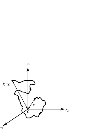
Figure 1: The $D$-dimensional Bessel process $X^{x}(t)$ is defined as the radial part of the BM in the $D$-dimensional space. The initial value $x$ of the Bessel process is the distance between the origin and the position from which the BM is started.

By this definition, $X^{x}(t)$ is a functional of $D$-tuples of stochastic processes $\{B^{x_{i}}_{i}(t)\}_{i=1}^{D}$. In order to describe the statistics of a function of several random variables, we have to see ‘propagation of error’. For stochastic processes, by Itô’s formula we can readily obtain an equation for the stochastic process that is defined as a functional of several stochastic processes. In the present case, we have the following equation,

$$dX^{x}(t)=dB(t)+\frac{D-1}{2}\frac{dt}{X^{x}(t)},\quad t\in[0,\infty),\quad x>0.$$ (1.6)

The first term of the RHS, $dB(t)$, denotes the infinitesimal increment of a one-dimensional standard BM starting from the origin at time $t=0$, $B(t)=B^{0}(t)$. It should be noted that $B(t)$ is a different BM from any $B^{x_{i}}_{i}(t),1\leq i\leq D$, which were used to define $X^{x}(t)$ in Eq.(1.5). Here we assume $X^{x}(t)>0$. Then, if $D>1$, for an infinitesimal increment of time $dt>0$, the second term in the RHS of (1.6) is positive. It means that there is a drift to increase the value of $X^{x}(t)$. This drift term is increasing in $D$ and decreasing in $X^{x}(t)$. Since as $X^{x}(t)\searrow 0$, the drift term $\nearrow\infty$, it seems that a ‘repulsive force’ is acting to the $D$-dimensional BM, $\mbox{\boldmath$B$}^{\mbox{\boldmath$x$}}(t),|\mbox{\boldmath$x$}|>0$ to keep the distance from the origin positive, $X^{x}(t)=|\mbox{\boldmath$B$}^{\mbox{\boldmath$x$}}(t)|>0$, in order to avoid collision of the Brownian particle at the origin. Such a differential equation as (1.6), which involves random fluctuation term and drift term is called a stochastic differential equation (SDE).

What is the origin of the repulsive force between the $D$-dimensional BM and the origin? Why $\mbox{\boldmath$B$}^{\mbox{\boldmath$x$}}(t)$ starting from a point $\mbox{\boldmath$x$}\not=0$ does not want to return to the origin ? Why the strength of the outward drift is increasing in the dimension $D>1$ ?

There is no positive reason for $\mbox{\boldmath$B$}^{\mbox{\boldmath$x$}}(t)$ to avoid visiting the origin, since by definition (1.4) all components $B^{x_{i}}_{i}(t)$ enjoy independent BMs. As the dimension of space $D$ increases, however, the possibility not to visit the origin (or the fixed special point) increases, since among $D$ directions in the space only one direction is toward the origin (or the fixed special point) and other $D-1$ directions are orthogonal to it. If one know the second law of thermodynamics, which is also called the law of increasing entropy, one will understand that we would like to say here that the repulsive force acting from the origin to the Bessel process is an ‘entropy force’. (Note that the physical dimension of entropy [J/K] is different from that of force [J/m].) Anyway, the important fact is that, while the variance (quadratic variation) of the standard BM is fixed as $(dB(t))^{2}=dt$ for a given $dt>0$, the strength of repulsive drift is increasing in $D$. Then, the return probability of $X^{x}(t),x>0$ to the origin should be a decreasing function of $D$.

Let $p^{(D)}_{t}(y|x)$ be the transition probability density of the $D$-dimensional Bessel process. We can show that, for any $y\in\mathbb{R}_{+}$, $u^{(D)}_{t}(x)\equiv p^{(D)}_{t}(y|x),x>0$ solves the following partial differential equation (PDE)

$$\frac{\partial}{\partial t}u^{(D)}_{t}(x)=\frac{1}{2}\frac{\partial^{2}}{\partial x^{2}}u^{(D)}_{t}(x)+\frac{D-1}{2x}\frac{\partial}{\partial x}u^{(D)}_{t}(x)$$ (1.7)

under the initial condition $u_{0}^{(D)}(x)=\delta(x-y)$, which is called the backward Kolmogorov equation for the $D$-dimensional Bessel process. We can see clear correspondence between the SDE (1.6) and the PDE (1.7). As shown by (1.3), the BM term, $dB(t)$, in (1.6) is mapped to the diffusion term $(1/2)\partial^{2}u^{(D)}_{t}(x)/\partial x^{2}$ in (1.7). In (1.7) the drift term is given by using the spatial derivative $\partial/\partial x$ representing the outward drift with the coefficient $(D-1)/2x$ corresponding to the factor $(D-1)/(2X^{x}(t))$ of the second term in (1.6). The solution is given by

$$p^{(D)}_{t}(y|x)=\left\{\begin{array}[]{ll}\displaystyle{\frac{1}{t}\frac{y^{\nu+1}}{x^{\nu}}e^{-(x^{2}+y^{2})/2t}I_{\nu}\left(\frac{xy}{t}\right)},&\quad t>0,x>0,y\geq 0,\cr\displaystyle{\frac{y^{2\nu+1}}{2^{\nu}t^{\nu+1}\Gamma(\nu+1)}e^{-y^{2}/2t}},&\quad t>0,x=0,y\geq 0\cr&\cr\delta(y-x),&\quad t=0,x,y\geq 0,\end{array}\right.$$ (1.8)

where $I_{\nu}(z)$ is the modified Bessel function of the first kind defined by

$$I_{\nu}(z)=\sum_{n=0}^{\infty}\frac{1}{\Gamma(n+1)\Gamma(n+1+\nu)}\left(\frac{z}{2}\right)^{2n+\nu}$$ (1.9)

with the gamma function $\Gamma(z)=\int_{0}^{\infty}e^{-u}u^{z-1}du$, and the index $\nu$ is specified by the dimension $D$ as

$$\nu=\frac{D-2}{2}\quad\Longleftrightarrow\quad D=2(\nu+1).$$ (1.10)

This fact that $p^{(D)}_{t}(y|x)$ is expressed by using $I_{\nu}(z)$ gives the reason why the process $X^{x}(t)$ is called the Bessel process.

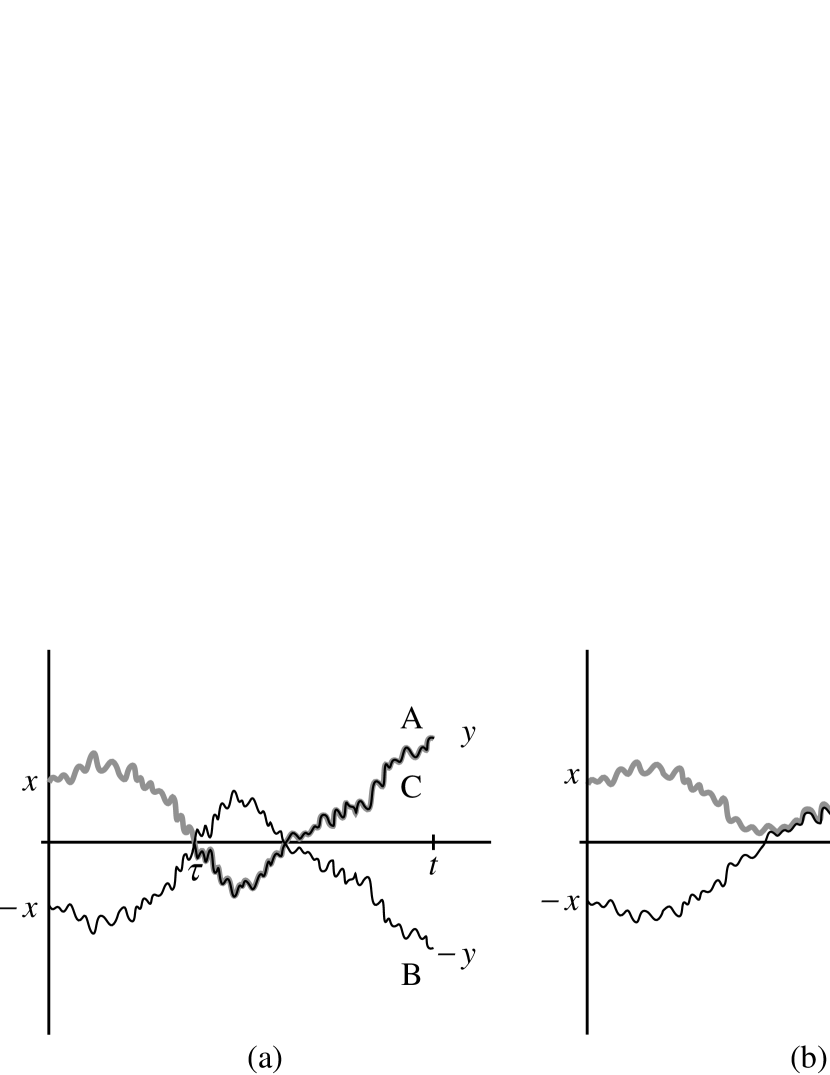
Figure 2: (a) One realization of Brownian path from $x>0$ to $y>0$ is drawn (path A), which visits the nonpositive region $\mathbb{R}_{-}\equiv\{x\in\mathbb{R}:x\leq 0\}$. The path B is a mirror image of path A with respect to the origin $x=0$, which is running from $-x<0$ to $-y<0$. The first time when the path B hits the origin is denoted by $\tau$. The path C is a combination of a part of path B up to time $\tau$ and a part of path A after $\tau$ such that it runs from $-x<0$ to $y>0$. There establishes bijection between path A and path C, which have the same weight as Brownian paths. Since the Brownian path A contributes to $p_{t}(y|x)$ and the Brownian path B does to $p_{t}(y|-x)$, such a path from $x>0$ to $y>0$ visiting $\mathbb{R}_{-}$ is cancelled in $p_{t}^{\rm abs}(y|x)$. (b) Each path, which does not visit $\mathbb{R}_{-}$, gives positive contribution to $p_{t}^{\rm abs}(y|x)$, since in this case the weight of Brownian path A contributing to $p_{t}(y|x)$ is bigger than that of Brownian path C contributing $p_{t}(y|-x)$. In summary, $p_{t}^{\rm abs}(y|x)=p_{t}(y|x)-p_{t}(y|-x)$ gives the total weight of Brownian paths, which do not hit the origin and thus are not absorbed at the wall at the origin.

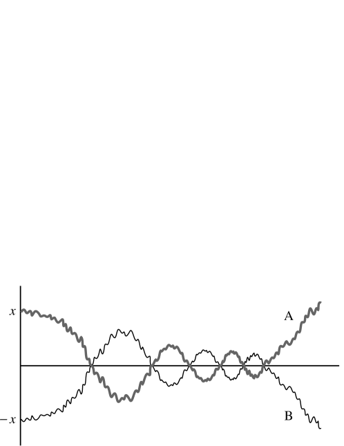
Figure 3: The one-dimensional BM visits the origin frequently. For a Brownian path starting from $x>0$ (path A), its mirror image with respect to the origin is drawn (path B), which starts from $-x<0$. If we observe the motion only in the nonnegative region $\mathbb{R}_{+}$, the superposition of Brownian paths A and B gives a path of a reflecting BM, where a reflecting wall is put at the origin.

When $D=3$, $\nu=1/2$ by (1.10), and we can use the equality $I_{1/2}(z)=\sqrt{2/\pi z}\sinh z=(e^{z}-e^{-z})/\sqrt{2\pi z}$. Then (1.8) gives

$$p_{t}^{(3)}(y|x)=\frac{y}{x}\Big{\{}p_{t}(y|x)-p_{t}(y|-x)\Big{\}}$$ (1.11)

for $t>0,x>0,y\geq 0$, where $p_{t}(y|x)$ is the transition probability density (1.1) of BM. If we put $p^{\rm abs}_{t}(y|x)=p_{t}(y|x)-p_{t}(y|-x)$, we see $p^{\rm abs}_{t}(0|x)=0$ for any $x>0$, since BM is a symmetric process.

As shown by Fig.2, $p^{\rm abs}_{t}(y|x),x,y\geq 0$, gives the transition probability density of the absorbing BM, in which an absorbing wall is put at the origin and, if the Brownian particle starting from $x>0$ arrives at the origin, it is absorbed there and the motion is stopped. By absorption, the total mass of paths from $x>0$ to $y>0$ is then reduced. The factor $y/x$ appearing in (1.11) is for renormalization so that $\int_{\mathbb{R}_{+}}p^{(3)}_{t}(y|x)dy=1,\forall t>0,\forall x>0$. We regard this renormalization procedure from $p^{\rm abs}_{t}$ to $p^{(3)}_{t}$ as a transformation. Since $x$ is a one-dimensional harmonic function in a rather trivial sense $\Delta^{(1)}x\equiv d^{2}x/dx^{2}=0$, we say that the three-dimensional Bessel process is an harmonic transform ($h$-transform) of the one-dimensional absorbing BM in the sense of Doob [14]. This implies the equivalence between the three-dimensional Bessel process and ‘the one-dimensional BM conditioned to stay positive’. We will discuss such equivalence of processes in Section 2 more detail. Here we put emphasize the fact that $p^{(3)}_{t}(0|x)=0,\forall x>0$. It means that the three-dimensional Bessel process does not visit the origin. When $D=3$, the outward drift is strong enough to avoid any visit to the origin. Moreover, we can prove that for any $x>0$, $X^{x}(t)\to\infty$ as $t\to\infty$ w.p.1 and we say the process is transient.

When $D=1$, $\nu=-1/2$ by (1.10) and we use the equality $I_{-1/2}(z)=\sqrt{2/\pi z}\cosh z=(e^{z}+e^{-z})/\sqrt{2\pi z}$. In this case (1.8) gives

$$p^{(1)}_{t}(y|x)=p_{t}(y|x)+p_{t}(y|-x)$$ (1.12)

for $t>0,x,y\geq 0$. As shown by Fig.3, (1.12) means the equivalence between the one-dimensional Bessel process and ‘the one-dimensional BM with a reflecting wall at the origin’. This is of course a direct consequence of the definition of Bessel process (1.5), since it gives $X^{x}(t)=|B^{x}(t)|$ in $D=1$. The important fact is that the one-dimensional BM starting from $x\not=0$ visits the origin frequently and we say that the one-dimensional Bessel process is recurrent. (Remark that in Eqs. (1.6) and (1.7), the drift terms vanish when $D=1$. So we have to assume the reflecting boundary condition at the origin when we discuss the one-dimensional Bessel process instead of the one-dimensional BM.)

Now the following question is addressed: At which dimension the Bessel process changes its property from recurrent to transient ?

Before answering this question, here we would like to extend the setting of the question. Originally, the Bessel process was defined by (1.5) for $D\in\mathbb{N}$. We find that, however, the modified Bessel function (1.9) is an analytic function of $\nu$ for all values of $\nu$. So we will be able to define the Bessel process for any positive value of dimension $D>0$ as the diffusion process in $\mathbb{R}_{+}$ such that the transition probability density function is given by (1.8), where the index $\nu>-1$ is determined by (1.10) for each value of $D$. (In the SDE, (1.6), we assume the reflecting boundary condition at the origin for $0<D<2$.) Now we introduce an abbreviation BES^(D) for the $D$-dimensional Bessel process, $D>0$ .

For BES^(D) starting from $x>0$, denote its first visiting time at the origin by

$$T^{x}=\inf\{t>0:X^{x}(t)=0\}.$$ (1.13)

The answer of the above question is given by the following theorem.

Theorem 1.1

(i)  $D\geq 2\quad\Longrightarrow\quad T^{x}=\infty,^{\forall}x>0$, w.p.1.

(ii)  $D>2\quad\Longrightarrow\quad\displaystyle{\lim_{t\to\infty}}X^{x}(t)=\infty,\,^{\forall}x>0$, w.p.1, i.e. the process is transient.

(iii)  $D=2\quad\Longrightarrow\quad\displaystyle{\inf_{t>0}}\,X^{x}(t)=0,\,^{\forall}x>0$, w.p.1 D
That is, BES⁽²⁾ starting from $x>0$ does not visit the origin, but it can visit any neighbor of the origin.

(iv)  $D<2\quad\Longrightarrow\quad T^{x}<\infty,\,^{\forall}x>0$, w.p.1, i.e. the process is recurrent.

1.3 Bessel flow and Cardy’s formula

In the previous subsection, we have defined the BES^(D) for positive continuous values of dimension $D>0$ and studied dependence of the probability law of process on $D$. Theorem 1.1 states that the two-dimension is a critical dimension,

$$D_{\rm c}=2,$$

for competition between the two effects acting the Bessel process, the ‘random force’ (the martingale term) and the ‘entropy force’ (the drift term) in (1.6) and (1.7): when $D>D_{\rm c}$, the latter dominates the former and the process becomes transient, and when $D<D_{\rm c}$, the former is relevant and recurrence to the origin of the process is realized frequently.

Here we show that there is another critical dimension,

$$\overline{D}_{\rm c}=\frac{3}{2}.$$

In order to characterize the transition at $\overline{D}_{\rm c}$, we have to investigate dependence of the behavior of $X^{x}(t)$ on initial value $x>0$. We call the one-parameter family $\{X^{x}(t)\}_{x>0}$ the Bessel flow for each fixed $D>0$.

For $0<x<y$, we trace the motions of two BES^(D)’s starting from $x$ and $y$ by solving (1.6) using the common BM, $B(t),t\geq 0$,

$$X^{x}(t)=x+B(t)+\frac{D-1}{2}\int_{0}^{t}\frac{ds}{X^{x}(s)},$$

$$X^{y}(t)=y+B(t)+\frac{D-1}{2}\int_{0}^{t}\frac{ds}{X^{x}(s)},\quad t\geq 0.$$

By considering the coupling of the two processes, we can show that

$$x<y\quad \Longrightarrow \quad X^{x}(t)<X^{y}(t),\quad t<T^{x}\quad\mbox{w.p.1}$$

$$\Longrightarrow \quad T^{x}\leq T^{y}\quad\mbox{w.p.1}.$$

The interesting fact is that in the intermediate fractional dimensions, $\overline{D}_{\rm c}<D<D_{\rm c}$, it is possible to see the coincide $T^{x}=T^{y}$ even for $x<y$. See Fig.4.

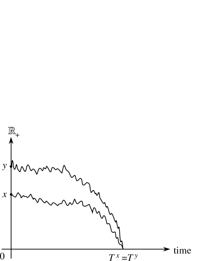
Figure 4: In the intermediate fractional dimensions, $3/2<D<2$, there is a positive probability that two Bessel processes starting from different initial positions, $0<x<y<\infty$, return to the origin simultaneously, $T^{x}=T^{y}$.

Theorem 1.2

For $0<x<y<\infty$,

(i)  $D\leq 3/2\quad\Longrightarrow\quad T^{x}<T^{y}\quad\mbox{w.p.1}$.

(ii)  $3/2<D<2\quad\Longrightarrow\quad{\rm P}(T^{x}=T^{y})>0$.

Theorem 1.2 (ii) is obtained by proving that, for $0<x<y<\infty,3/2<D<2$, the event

$$\sup_{t<T^{x}}\frac{X^{y}(t)-X^{x}(t)}{X^{x}(t)}<\infty$$ (1.14)

occurs with positive probability. If (1.14) holds, ${}^{\exists}c<\infty$ s.t. $X^{y}(t)\leq(1+c)X^{x}(t),0<t<T^{x}$ and thus $X^{x}(t)=0\Longrightarrow X^{y}(t)=0\Longrightarrow T^{x}=T^{y}$. We can confirm that the difference between the event $\{T^{x}=T^{y}\}$ and the event (1.14) has probability zero (see Section 1.10 in [60]).

A striking fact is the following exact formula: for $3/2<D<2,0<x<y<\infty$,

$${\rm P}(T^{x}=T^{y}) = 1-\frac{\Gamma(D-1)}{\Gamma(2(D-1))\Gamma(2-D)}\left(\frac{y-x}{y}\right)^{2D-3}$$ (1.15)

$$\quad\times F\left(2D-3,D-1,2(D-1);\frac{y-x}{y}\right),$$

where $F(\alpha,\beta,\gamma;z)$ is Gauss’ hypergeometric function

$$F(\alpha,\beta,\gamma;z)=\sum_{i=0}^{\infty}\frac{(\alpha)_{i}(\beta)_{i}}{(\gamma)_{i}}\frac{z^{i}}{i!}$$

with the Pochhammer symbol $(c)_{i}=c(c+1)\cdots(c+i-1)$. If we set $D=5/3$, (1.15) becomes a version of exact formula for a physical quantity called ‘crossing probability’ that Cardy derived in a critical percolation model [10, 11]. Cardy’s formula has been extended in the context of SLE (see Section 6.7 of [60]), but I think that this exact formula for the Bessel flow can be also called Cardy’s formula.

1.4 Schramm-Loewner evolution (SLE) as complexification of Bessel flow

Now we consider an extension of the Bessel flow $X^{x}(t)$ defined on $\mathbb{R}_{+}$ to flow on the upper-half complex-plane $\mathbb{H}=\{z=x+\sqrt{-1}y:x\in\mathbb{R},y>0\}$ and its boundary $\partial\mathbb{H}=\mathbb{R}$. We set $Z^{z}(t)=X^{z}(t)+\sqrt{-1}Y^{z}(t)\in\overline{\mathbb{H}}\setminus\{0\}=\mathbb{H}\cup\mathbb{R}\setminus\{0\},t\geq 0$ and complexificate (1.6) as

$$dZ^{z}(t)=dB(t)+\frac{D-1}{2}\frac{dt}{Z^{z}(t)},\quad t\in[0,\infty)$$ (1.16)

with the initial condition

$$Z^{z}(0)=z=x+\sqrt{-1}y\in\overline{\mathbb{H}}\setminus\{0\}.$$

The crucial point of this complexification of the Bessel flow is that the BM remains real. Then, there is asymmetry between the real part and the imaginary part of the flow in $\mathbb{H}$,

$$dX^{z}(t)=dB(t)+\frac{D-1}{2}\frac{X^{z}(t)}{(X^{z}(t))^{2}+(Y^{z}(t))^{2}}dt,$$ (1.17)

$$dY^{z}(t)=-\frac{D-1}{2}\frac{Y^{z}(t)}{(X^{z}(t))^{2}+(Y^{z}(t))^{2}}dt.$$ (1.18)

Assume $D>1$. Then as indicated by the minus sign in the RHS of (1.17), the flow is downward in $\overline{\mathbb{H}}$. If the flow goes down and arrives at the real axis, the imaginary part vanishes, $Y^{z}(t)=0$, and Eq.(1.17) is reduced to be the same equation as Eq.(1.6) for the BES^(D), which is now considered for $\mathbb{R}\setminus\{0\}$. If $D>2$, by Theorem 1.1 (ii), the flow on $\mathbb{R}\setminus\{0\}$ is asymptotically outward, $X^{x}\to\pm\infty$ as $t\to\infty$. Therefore, the flow on $\overline{\mathbb{H}}$ will be described as shown by Fig.5. The behavior of flow should be, however, more complicated when $\overline{D}_{\rm c}=3/2<D<D_{\rm c}$ and $1<D<\overline{D}_{\rm c}$.

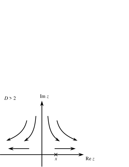
Figure 5: A schematic picture of ‘SLE flow’ on $\overline{\mathbb{H}}\setminus\{0\}$ for $D>2$.

For $z\in\overline{\mathbb{H}}\setminus\{0\},t\geq 0$, let

$$g_{t}(z)=Z^{z}(t)-B(t).$$ (1.19)

Then, Eq.(1.16) is written as follows:

$$\frac{d}{dt}g_{t}(z)=\frac{D-1}{2}\frac{1}{g_{t}(z)+B(t)},\quad t\geq 0,$$ (1.20)

with the initial condition $g_{0}(z)=z\in\overline{\mathbb{H}}\setminus\{0\}$. For each $z\in\overline{\mathbb{H}}\setminus\{0\}$, set

$$T^{z}=\inf\{t>0:g_{t}(z)+B(t)=0\},$$ (1.21)

then the solution of Eq.(1.20) exists up to time $T^{z}$. For $t\geq 0$ we put

$$H_{t}=\{z\in\mathbb{H}:T^{z}>t\}.$$ (1.22)

This ordinary differential equation (1.20) involving the BM is nothing but the celebrated Schramm-Loewner evolution (SLE) [77, 60]. For each $t\geq 0$, the solution $g_{t}(z)$ of (1.20) gives a unique conformal transformation from $H_{t}$ to $\mathbb{H}$:

$$g_{t}(z):\quad H_{t}\to\mathbb{H},\quad\mbox{conformal}$$

such that

$$g_{t}(z)=z+\frac{a(t)}{z}+{\cal O}\left(\frac{1}{|z|^{2}}\right),\quad z\to\infty$$

with

$$a(t)=\frac{D-1}{2}t.$$

Note that the inverse map $g_{t}^{-1}$ from $\mathbb{H}$ to $H_{t},t\geq 0$, is also conformal. For each $t\geq 0$, there exists a limit

$$\gamma(t)=\lim_{z\to 0,z\in\mathbb{H}}g_{t}^{-1}(z-B(t)),$$ (1.23)

and using basic properties of BM, we can prove that $\gamma=\gamma[0,\infty)\equiv\{\gamma(t):t\in[0,\infty)\}\in\overline{\mathbb{H}}$ is a continuous path w.p.1 running from $\gamma(0)=0$ to $\gamma(\infty)=\infty$ [74]. The path $\gamma$ obtained from the SLE with the parameter $D>1$ is called the SLE^(D) path .

The dependence on $D$ of the Bessel flow given by Theorems 1.1 and 1.2 is mapped to the feature of the SLE^(D) paths such that there are three phases.

[phase 1]   When $D\geq D_{\rm c}=2$, the SLE^(D) path is a simple curve, i.e., $\gamma(s)\not=\gamma(t)$ for any $0\leq s\not=t<\infty$, and $\gamma(0,\infty)\in\mathbb{H}$ (i.e., $\gamma(0,\infty)\cap\mathbb{R}=\emptyset$). In this phase,

$$H_{t}=\mathbb{H}\setminus\gamma(0,t],\quad t\geq 0.$$

For each $t\geq 0$, $g_{t}$ gives a map, which conformally erases a simple curve $\gamma(0,t]$ from $\mathbb{H}$, and the image of the tip $\gamma(t)$ of the SLE path is $-B(t)\in\mathbb{R}=\partial\mathbb{H}$ as given by (1.23). As shown by Fig.6, it implies that the ‘SLE flow’ in $\overline{\mathbb{H}}$ is downward in the vertical (imaginary-axis) direction and outward from the position $-B(t)$ in the horizontal (real-axis) direction. Since $Z^{z}(t)=g_{t}(z)+B(t)$ by (1.19), if we shift this figure by $B(t)$, we will have the similar picture to Fig.5 for the complexificated version of Bessel flow for $D>2$.

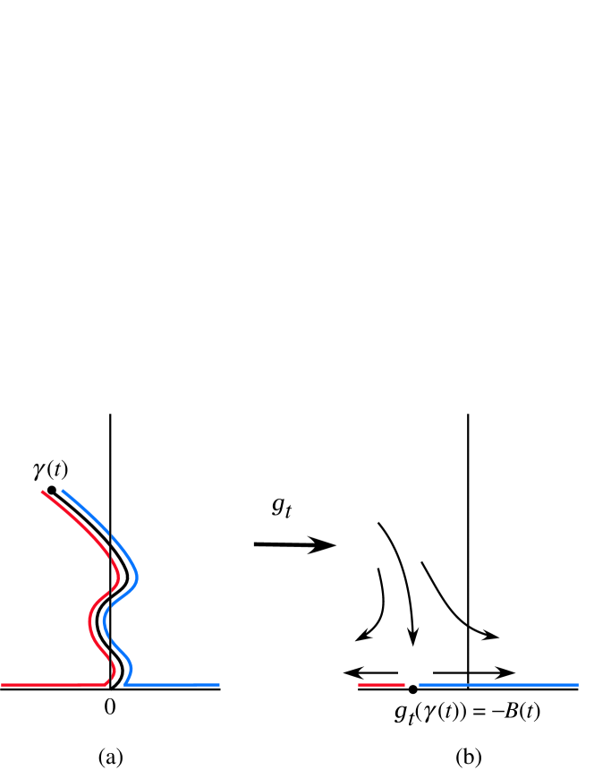
Figure 6: (a) When $D\geq 2$, the SLE^(D) path is simple. (b) By $g_{t}$, the SLE^(D) path is erased from $\mathbb{H}$. The tip of the SLE^(D) path $\gamma(t)$ is mapped to $g_{t}(\gamma(t))=-B(t)\in\mathbb{R}$. The flow associated by thus conformal transformation is shown by arrows.

[phase 2]   When $\overline{D}_{\rm c}=3/2<D<D_{\rm c}=2$, the SLE^(D) path can osculate the real axis, ${\rm P}(\gamma(0,t]\cap\mathbb{R}\not=\emptyset)>0,\forall t>0$. Fig.7 (a) illustrates the moment $t>0$ such that the tip of SLE^(D) path just osculates the real axis. The closed region encircled by the path $\gamma(0,t)$ and the line $[\gamma(t),0]\in\mathbb{R}$ is called an SLE hull at time $t$ and denoted by $K_{t}$. In this phase

$$H_{t}=\mathbb{H}\setminus K_{t},\quad t\geq 0.$$

That is, $g_{t}(z)$ is a map which erases conformally the SLE hull from $\mathbb{H}$. We can think that by this transformation all the points in $K_{t}$ are simultaneously mapped to a single point $-B(t)\in\mathbb{R}$, which is the image of the tip $\gamma(t)$. (We say that the hull $K_{t}$ is swallowed. See Fig.7 (b).) By definition (1.22), the moment when $K_{t}=\mathbb{H}\setminus H_{t}$ is swallowed is the time $T^{z}$ at which the equality $Z^{z}(t)=g_{t}(z)+B(t)=0$ holds ${}^{\forall}z\in K_{t}$. (Then the RHS of (1.20) diverges and all the points $z\in K_{t}$ are lost from the domain of the map $g_{t}$.) Theorem 1.2 (ii) states that, when $\overline{D}_{\rm c}<D<D_{\rm c}$, two BES^(D) starting from different points $0<x<y<\infty$ can simultaneously return to the origin. In the complexificated version, all $Z^{z}(t)$ starting from $z\in K_{t}$ can arrive at the origin simultaneously (i.e., they are all swallowed).

Osculation of the SLE path with $\mathbb{R}$ means that the SLE path has loops. Figure 8 (a) shows the event that the SLE path makes a loop at time $t>0$. The SLE hull $K_{t}$ consists of the closed region encircled by the loop and the segment of the SLE path between the origin and the osculating point, and it is completely erased by the conformal transformation $g_{t}$ to $\mathbb{H}$ as shown by Fig.8(b). Let $0<s<t$ and consider the map $g_{s}$, which is the solution of (1.20) at time $s$. Assume that $\gamma(s)$ is located on the loop part of $\gamma[0,t]$ as shown by Fig.8(a). The segment $\gamma[0,s]$ of the SLE path is mapped by $g_{s}$ to a part of $\mathbb{R}$. Since $\gamma(t)$ osculates a point in $\gamma[0,s]$, its image $g_{s}(\gamma(t))$ should osculate the real axis $\mathbb{R}$ as shown by Fig.8(c). Since $g_{s}^{-1}$ is uniquely determined from $g_{s}$, the above argument can be reversed. Then equivalence between osculation of the SLE path with $\mathbb{R}$ and self-intersection of the SLE path is concluded. In this intermediate phase $\overline{D}_{\rm c}<D<D_{\rm c}$,

SLE^(D) path $$\gamma$$ is self-intersecting, and

$$\bigcup_{t>0}\overline{K_{t}}=\overline{\mathbb{H}}\quad\mbox{but}\quad\gamma[0,\infty)\cap\mathbb{H}\not=\mathbb{H}\quad\mbox{w.p.1}.$$

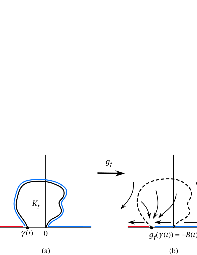
Figure 7: (a) When $3/2<D<2$, the SLE^(D) path can osculate the real axis. The SLE hull is denoted by $K_{t}$. (b) The SLE hull $K_{t}$ is swallowed. It means that all the points in $K_{t}$ are simultaneously mapped to a single point $-B(t)\in\mathbb{R}$, which is the image of the tip of the SLE^(D) path $\gamma(t)$.

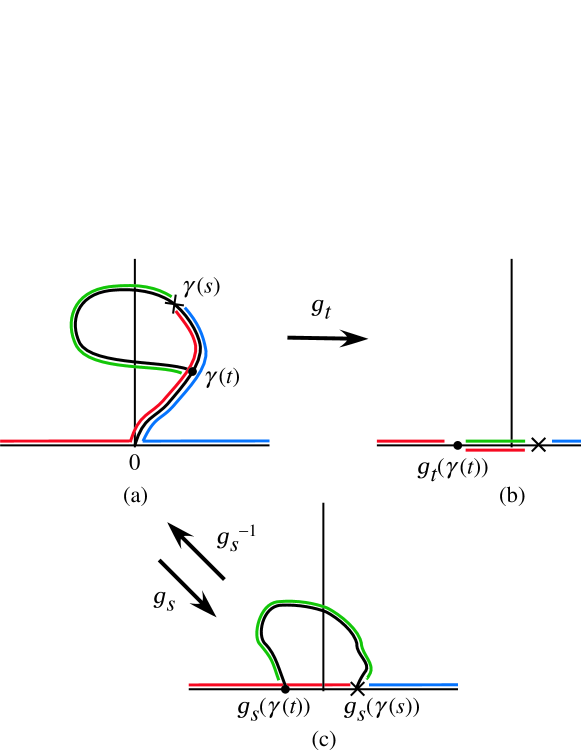
Figure 8: The event that the SLE^(D) path osculates $\mathbb{R}$ is equivalent with the event that the SLE^(D) path makes a loop.

[phase 3]   When $1<D\leq\overline{D}_{\rm c}=3/2$, Theorem 1.2 (i) states for the Bessel flow that the ordering $T^{x}<T^{y}$ is conserved for any $0<x<y$. It implies that in this phase the SLE path should be a space-filling curve;

$$\gamma[0,\infty)=\overline{\mathbb{H}}.$$

(Otherwise, swallow of regions occurs, contradicting Theorem 1.2 (i).)

Figure 9 summarizes the three phases of SLE paths.

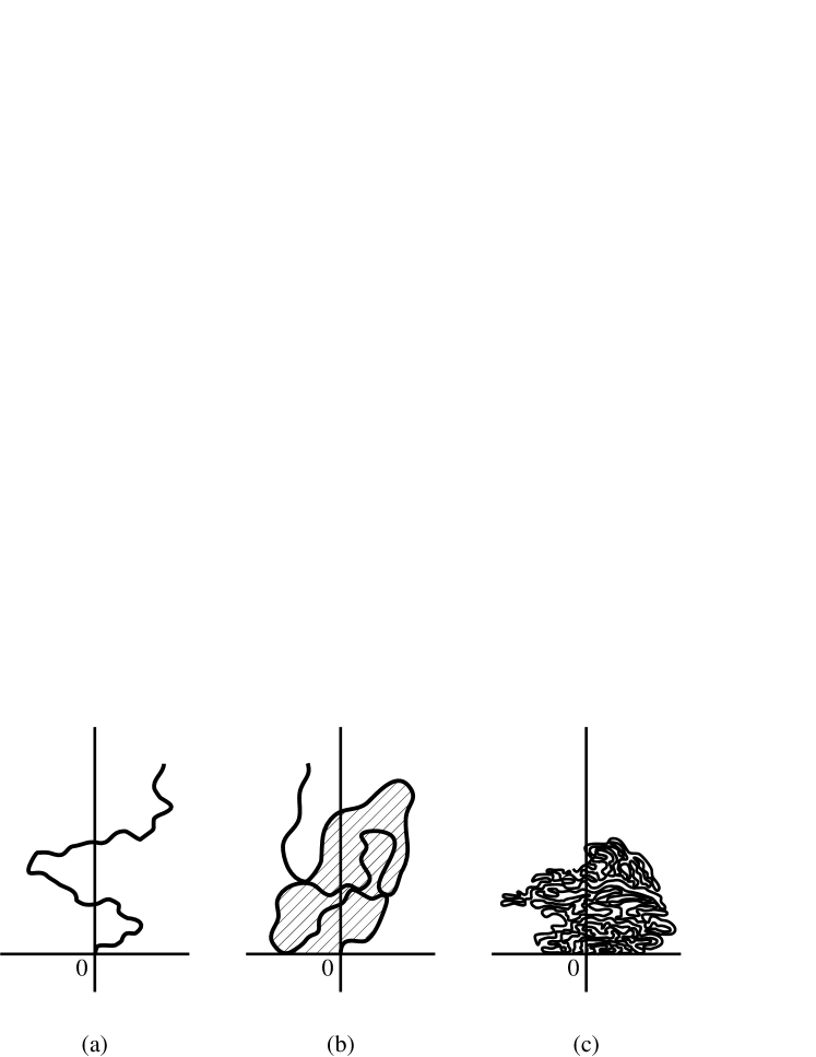
Figure 9: Schematic pictures of SLE^(D) paths in (a) phase 1 ($D\geq D_{\rm c}=2$), (b) phase 2 ($\overline{D}_{\rm c}=3/2<D<D_{\rm c}=2$), and (c) phase 3 ($1<D\leq\overline{D}_{\rm c}=3/2$).

By complexification of Bessel flow, we can discuss flows on a two-dimensional plane $\overline{\mathbb{H}}$. By this procedure random curves (the SLE paths) are generated in the plane. The SLE paths are fractal curves and their Hausdorff dimensions $d_{\rm H}^{(D)}$ are determined by Beffara [1]. We note that a reciprocity relation is found between $D$ and $d_{\rm H}^{(D)}$;

$$(D-1)(d_{\rm H}^{(D)}-1)=\frac{1}{2},\quad D\geq\overline{D}_{\rm c}=\frac{3}{2}.$$ (1.24)

(In the phase 3, $D\leq\overline{D}_{\rm c}=3/2$, $d_{\rm H}^{(D)}\equiv 2$.)

Remark that the SLE map $\gamma_{t}$ as well as the SLE path $\gamma$ are functionals of the BM. Therefore, we have statistical ensembles of random curves $\{\gamma\}$ in the probability space $(\Omega,{\cal F},{\rm P})$. The important consequence from the facts that the BM is a strong Markov process with independent increments and $g_{t}$ gives a conformal transformation is that the statistics of $\{\gamma\}$ has a kind of stationary Markov property (called the domain Markov property) and conformal invariance with respect to transformation of the domain in which the SLE path $\gamma$ is defined [60].

The highlight of the theory of SLE would be that, if the value $D$ is properly chosen, the statistics of $\{\gamma\}$ realizes that of the scaling limit of important statistical mechanics model exhibiting critical phenomena and fractal structures defined on an infinite discrete lattice. The following is a list of the correspondence between the SLE^(D) paths with specified values of $D$ and the scaling limits of models studied in statistical mechanics and fractal physics .

SLE^(3/2) $$\Longleftrightarrow$$ uniform spanning tree[62]

SLE^(5/3) $$\Longleftrightarrow$$ critical percolation model

(percolation exploration process)[80]

SLE⁽²⁾ $$\Longleftrightarrow$$ Gaussian free surface model (contour line)[78]

SLE^(7/3) $$\Longleftrightarrow$$ critical Ising model (Ising interface)[81]

SLE^(5/2) $$\Longleftrightarrow$$ self-avoiding walk [conjecture]

SLE⁽³⁾ $$\Longleftrightarrow$$ loop-erased random walk[62]

1.5 Dyson’s BM model as multivariate extension of Bessel process

Here we consider stochastic motion of two particles $(X_{1}(t),X_{2}(t))$ in one dimension $\mathbb{R}$ satisfying the following SDEs,

$$dX_{1}(t)=dB_{1}(t)+\frac{\beta}{2}\frac{dt}{X_{1}(t)-X_{2}(t)}$$

$$dX_{2}(t)=dB_{2}(t)+\frac{\beta}{2}\frac{dt}{X_{2}(t)-X_{1}(t)}\quad t\geq 0,$$ (1.25)

with the initial condition $X_{1}(0)<X_{2}(0)$, where $B_{1}(t)$ and $B_{2}(t)$ are independent one-dimensional standard BMs and $\beta>0$ is a ‘coupling constant’ of the two particles. The second terms in (1.25) represent the repulsive force acting between two particles, which is proportional to the inverse of distance $X_{2}(t)-X_{1}(t)$ of the two particles. Since it is a central force (i.e., depending only on distance, and thus symmetric for two particles), the ‘center of mass’ $X_{\rm c}(t)\equiv(X_{2}(t)+X_{1}(t))/2$ is proportional to a BM; $X_{\rm c}(t)\stackrel{{\scriptstyle\rm d}}{{=}}B(t)/\sqrt{2}\stackrel{{\scriptstyle\rm d}}{{=}}B(t/2),^{\forall}t\geq 0$, where $B(t)$ is a one-dimensional standard BM different from $B_{1}(t)$ and $B_{2}(t)$ and the symbol $\stackrel{{\scriptstyle\rm d}}{{=}}$ denotes the equivalence in distribution. (Note that variance (quadratic variation) $(dX_{\rm c}(t))^{2}=\{(dB_{1}(t)+dB_{2}(t))/2\}^{2}=dt/2$, since $(dB_{1}(t))^{2}=(dB_{2}(t))^{2}=dt$ and $dB_{1}(t)dB_{2}(t)=0$.) On the other hand, we can see that the relative coordinate defined by $X_{\rm r}(t)\equiv(X_{2}(t)-X_{1}(t))/\sqrt{2}$ satisfies the SDE

$$dX_{\rm r}(t)=d\widetilde{B}(t)+\frac{\beta}{2}\frac{dt}{X_{\rm r}(t)},\quad t\geq 0,$$

where $\widetilde{B}(t)$ is a BM different from $B_{1}(t),B_{2}(t),B(t)$. It is nothing but the SDE for BES^(D) with $D=\beta+1$.

Dyson [16] introduced $N$-particle systems of interacting BMs in $\mathbb{R}$ as a solution $\mbox{\boldmath$X$}(t)=(X_{1}(t),X_{2}(t),\dots,X_{N}(t))$ of the following system of SDEs,

$$dX_{i}(t)=dB_{i}(t)+\frac{\beta}{2}\sum_{1\leq j\leq N:j\not=i}\frac{dt}{X_{i}(t)-X_{j}(t)},\quad t\in(0,\tau),\quad i=1,2,\dots,N,$$ (1.26)

where $\{B_{i}(t)\}_{i=1}^{N}$ are independent one-dimensional standard BMs and we define

$$\sigma_{ij}=\inf\{t\geq 0:X_{i}(t)\not=X_{j}(t)\},\quad 1\leq i<j\leq N,$$

$$\tau_{ij}=\inf\{t>\sigma_{ij}:X_{i}(t)=X_{j}(t)\},\quad 1\leq i<j\leq N,$$

$$\qquad\qquad\tau=\min_{1\leq i<j\leq N}\tau_{ij}.$$

It is called Dyson’s BM model with parameter $\beta$ [65, 22]. As shown above, the $N=2$ case of Dyson’s BM model is a coordinate transformation of the pair of a (time-change of) BM and BES^(β+1). In this sense, Dyson’s BM model can be regarded as a multivariate (multi-dimensional) extension of BES${}^{(\beta+1)},\beta>0$ . In particular, we will characterize Dyson’s BM model with $\beta=2$ as an extension of the three-dimensional Bessel process, BES⁽³⁾, in Section 2.

2 Two aspects of the Dyson model

In this section, we study the special case of Dyson’s BM model with parameter $\beta=2$. We call this special case simply the Dyson model [48]. As shown above, the case $\beta=2$ corresponds to the case $D=3$ of Bessel process. In Sect.1.2, we have shown that BES⁽³⁾ has two aspects; (Aspect 1) as a radial coordinate of three-dimensional BM, and (Aspect 2) as a one-dimensional BM conditioned to stay positive. We show that the Dyson model inherits these two aspects from BES⁽³⁾ [47].

2.1 The Dyson model as eigenvalue process

Dyson introduced the process (1.26) with $\beta=1,2$, and 4 as the eigenvalue processes of matrix-valued BMs in the Gaussian orthogonal ensemble (GOE), the Gaussian unitary ensemble (GUE), and the Gaussian symplectic ensemble (GSE) [16, 65, 22] .

For $\beta=2$ with given $N\in\mathbb{N}$, we prepare $N$-tuples of one-dimensional standard BMs $\{B_{ii}^{x_{i}}\}_{j=1}^{N}$, each of which starts from $x_{i}\in\mathbb{R}$, $N(N-1)/2$-tuples of pairs of BMs $\{B_{ij},\widetilde{B}_{ij}\}_{1\leq i<j\leq N}$, all of which start from the origin, where the totally $N+2\times N(N-1)/2=N^{2}$ BMs are independent from each other. Then consider an $N\times N$ Hermitian-matrix-valued BM .

$${\cal H}^{\mbox{\boldmath$x$}}(t)=\left(\begin{array}[]{cccc}B_{11}^{x_{1}}(t)&\displaystyle{\frac{B_{12}(t)+\sqrt{-1}\widetilde{B}_{12}(t)}{\sqrt{2}}}&\cdots&\displaystyle{\frac{B_{1N}(t)+\sqrt{-1}\widetilde{B}_{1N}(t)}{\sqrt{2}}}\cr\displaystyle{\frac{B_{12}(t)-\sqrt{-1}\widetilde{B}_{12}(t)}{\sqrt{2}}}&B_{22}^{x_{2}}(t)&\cdots&\displaystyle{\frac{B_{2N}(t)+\sqrt{-1}\widetilde{B}_{2N}(t)}{\sqrt{2}}}\cr\cdots&\cdots&\cdots&\cdots\cr\displaystyle{\frac{B_{1N}(t)-\sqrt{-1}\widetilde{B}_{1N}(t)}{\sqrt{2}}}&\displaystyle{\frac{B_{2N}(t)-\sqrt{-1}\widetilde{B}_{2N}(t)}{\sqrt{2}}}&\cdots&B_{NN}^{x_{N}}(t)\end{array}\right).$$ (2.1)

By this definition, the initial state of this BM is given by the diagonal matrix

$${\cal H}^{\mbox{\boldmath$x$}}(0)={\rm diag}(x_{1},x_{2},\dots,x_{N}).$$ (2.2)

We assume $x_{1}\leq x_{2}\leq\cdots\leq x_{N}$.

Remember that when we introduced BES^(D) in Sect.1.2, we considered the $D$-dimensional vector-valued BM, (1.4), by preparing $D$-tuples of independent one-dimensional standard BMs for its elements. Since the dimension of the space ${\rm H}(N)$ of $N\times N$ Hermitian matrices is ${\rm dim}\,{\rm H}(N)=N^{2}$, we need $N^{2}$ independent BMs for elements to describe a BM in this space ${\rm H}(N)$.

Corresponding to calculating an absolute value of $\mbox{\boldmath$B$}^{\mbox{\boldmath$x$}}(t)$, by which BES^(D) was introduced as (1.5), here we calculate eigenvalues of ${\cal H}^{\mbox{\boldmath$x$}}(t)$. For any $t\geq 0$, there is a family of $N\times N$ unitary matrices $\{U(t)\}$ which diagonalize ${\cal H}^{\mbox{\boldmath$x$}}(t)$,

$$U(t)^{*}{\cal H}^{\mbox{\boldmath$x$}}(t)U(t)={\rm diag}(\lambda_{1}(t),\dots,\lambda_{N}(t)),\quad t\geq 0.$$

Let $\mathbb{W}_{N}^{\rm A}$ be the Weyl chamber of type A_N-1 defined by

$$\mathbb{W}_{N}^{\rm A}\equiv\{\mbox{\boldmath$x$}=(x_{1},x_{2},\dots,x_{N})\in\mathbb{R}^{N}:x_{1}<x_{2}<\cdots<x_{N}\}.$$

If we impose the condition $\mbox{\boldmath$\lambda$}(t)\equiv(\lambda_{1}(t),\dots,\lambda_{N}(t))\in\mathbb{W}_{N}^{\rm A},t\geq 0$, $U(t)$ is uniquely determined.

For each $t\geq 0$, $\lambda_{i}(t),1\leq i\leq N$ are functionals of $\{B_{ii}^{x_{i}}(t),B_{ij}(t),\widetilde{B}_{ij}\}_{1\leq i<j\leq N}$, and then, again we can apply Itô’s formula to take into account propagation of error correctly to derive SDEs for the eigenvalue process $\mbox{\boldmath$\lambda$}(t),t\geq 0$ [7, 8, 41]. The result is the following,

$$d\lambda_{i}(t)=dB_{i}^{x_{i}}(t)+\sum_{1\leq j\leq N:j\not=i}\frac{dt}{\lambda_{i}(t)-\lambda_{j}(t)},\quad t\in(0,\infty),\quad i=1,2,\dots,N,$$ (2.3)

where $\{B_{i}^{x_{i}}\}_{i=1}^{N}$ are independent BM different from the BMs used to define ${\cal H}^{\mbox{\boldmath$x$}}(t)$ by (2.1). It is indeed the $\beta=2$ case of (1.26) as derived by Dyson (originally not by such a stochastic calculus but by applying the perturbation theory in quantum mechanics) [16].

Now the correspondence is summarized as follows.

$$\begin{array}[]{lccl}{\mbox{\bf[Aspect 1]}}&&&\cr&\mbox{BES${}^{(3)}$}&\Longleftrightarrow&\mbox{radial coordinate of}\cr&&&\mbox{$D=3$ vector-valued BM}\cr&&&\cr&\mbox{the Dyson model}&\Longleftrightarrow&\mbox{eigenvalue process of}\cr&\mbox{with $N$ particles}&&\mbox{$N\times N$ Hermitian-matrix-valued BM}\end{array}$$

2.2 The Dyson model as noncolliding BM

Here we try to extend the formula (1.11) for BES⁽³⁾ to multivariate versions.

First we consider a set of two operations, identity ($\sigma_{1}=$ id) and reflection ($\sigma_{2}=$ ref), such that for $x\in\mathbb{R}$, $\sigma_{1}(x)=x$ and $\sigma_{2}(x)=-x$, and signatures are given as ${\rm sgn}(\sigma_{1})=1$ and ${\rm sgn}(\sigma_{2})=-1$, respectively. Then we have

$$p_{t}^{\rm abs}(y|x)=\sum_{\sigma\in\{{\rm id},{\rm ref}\}}{\rm sgn}(\sigma)p_{t}(y|\sigma(x)),\quad t\geq 0,\quad x,y,\in\mathbb{R}.$$ (2.4)

Next we consider a set of all permutations of $N$ indices $\{1,2,\dots,N\}$, which is denoted by ${\cal S}_{N}$, and put the following multivariate function

$$\sum_{\sigma\in{\cal S}_{N}}{\rm sgn}(\sigma)\prod_{i=1}^{N}p_{t}(y_{\sigma(i)}|x_{i})=\det_{1\leq i,j\leq N}\Big{[}p_{t}(y_{i}|x_{j})\Big{]}$$ (2.5)

of $\mbox{\boldmath$x$}=(x_{1},\dots,x_{N})\in\mathbb{W}_{N}^{\rm A}$ and $\mbox{\boldmath$x$}=(y_{1},\dots,y_{N})\in\mathbb{W}_{N}^{\rm A}$ with a parameter $t\geq 0$. Following the argument by Karlin and McGregor [34], we can prove that this determinant gives the transition probability density with duration $t$ from the state $x$ to the state $y$ of $N$-dimensional absorbing BM, $\mbox{\boldmath$B$}^{\mbox{\boldmath$x$}}(t)=(B_{1}^{x_{1}}(t),\dots,B_{N}^{x_{N}}(t))$, in a domain $\mathbb{W}_{N}^{\rm A}$, in which absorbing walls are put at the boundaries of $\mathbb{W}_{N}^{\rm A}$. Since the boundaries of $\mathbb{W}_{N}^{\rm A}$ are the hyperplanes $x_{i}=x_{j},1\leq i<j\leq N$, the Brownian particle $\mbox{\boldmath$B$}^{\mbox{\boldmath$x$}}(t)$ is annihilated, when any coincidence of the values of coordinates of $\mbox{\boldmath$B$}^{\mbox{\boldmath$x$}}(t)$ occurs. The ‘survival probability’ that the BM is not yet absorbed at the boundary is a monotonically decreasing function of time. If we regard the $i$-th coordinate $B_{i}^{x_{i}}(t)$ as the position of $i$-th particle on $\mathbb{R},1\leq i\leq N$, the state $\mbox{\boldmath$x$}\in\mathbb{W}_{N}^{\rm A}$ is considered to represent a configuration of $N$ particles on $\mathbb{R}$ such that a strict ordering $x_{1}<x_{2}<\cdots<x_{N}$ of positions is maintained, while the state absorbed at the boundary, $\mbox{\boldmath$x$}\in\partial\mathbb{W}_{M}^{\rm A}$, is a configuration in which collision occurs between some pair of neighboring pairs of particles; $1\leq^{\exists}i\leq N-1$, s.t. $x_{i}=x_{i+1}$. Since if such collision occurs, the process is totally annihilated, this many-particle system is called vicious walker model [20, 57, 32, 38, 33, 12].

As already noted below Eq.(1.11), $h_{1}(x)=x$ is a harmonic function in $(0,\infty)$ conditioned $\phi(0)=0$. Similarly, if we consider a harmonic function of $N$ variables

$$\Delta^{(N)}h_{N}(\mbox{\boldmath$x$})\equiv\sum_{i=1}^{N}\frac{\partial^{2}}{\partial x_{i}^{2}}h_{N}(\mbox{\boldmath$x$})=0$$ (2.6)

conditioned $h_{N}(\widehat{\mbox{\boldmath$x$}})=0,\,^{\forall}\widehat{\mbox{\boldmath$x$}}\in\partial\mathbb{W}_{N}^{\rm A}$, we will have the following product of differences

$$h_{N}(\mbox{\boldmath$x$})=\prod_{1\leq i<j\leq N}(x_{j}-x_{i}),$$ (2.7)

which is identified with the Vandermonde determinant $\det_{1\leq i,j\leq N}[x_{i}^{j-1}]$.

Combining above consideration, we put the following function

$$p_{t}^{N}(\mbox{\boldmath$y$}|\mbox{\boldmath$x$})=\frac{h_{N}(\mbox{\boldmath$y$})}{h_{N}(\mbox{\boldmath$x$})}\det_{1\leq i,j\leq N}\Big{[}p_{t}(y_{i}|x_{j})\Big{]},\quad t\geq 0,\quad\mbox{\boldmath$x$},\mbox{\boldmath$y$}\in\mathbb{W}_{N}^{\rm A}.$$ (2.8)

We can show that the factor $h_{N}(\mbox{\boldmath$y$})/h_{N}(\mbox{\boldmath$x$})$ provides an exact renormalization of the vicious walker model (the absorbing BM in $\mathbb{W}_{N}^{\rm A}$) to compensate any decay of total mass of the process by collision (by absorption at $\partial\mathbb{W}_{N}^{\rm A}$), and that (2.8) gives the transition probability density function for the $N$-particle system of one-dimensional BMs conditioned never to collide with each other forever (which we simply call the noncolliding BM) [25, 38, 39].

Moreover, by using the harmonicity (2.6), we can confirm that (2.8) satisfies the following partial differential equation,

$$\frac{\partial}{\partial t}p_{t}^{N}(\mbox{\boldmath$y$}|\mbox{\boldmath$x$})=\frac{1}{2}\Delta^{(N)}p_{t}^{N}(\mbox{\boldmath$y$}|\mbox{\boldmath$x$})+\sum_{1\leq i\not=j\leq N}\frac{1}{x_{i}-x_{j}}\frac{\partial}{\partial x_{i}}p_{t}^{N}(\mbox{\boldmath$y$}|\mbox{\boldmath$x$})$$ (2.9)

with the initial condition $p_{0}^{N}(\mbox{\boldmath$y$}|\mbox{\boldmath$x$})=\delta(\mbox{\boldmath$y$}-\mbox{\boldmath$x$})=\prod_{i=1}^{N}\delta(y_{i}-x_{i})$ [38]. It can be regarded as the backward Kolmogorov equation of the stochastic process with $N$ particles, $\mbox{\boldmath$X$}(t)=(X_{1}(t),\dots,X_{N}(t))$, which solves the system of SDEs,

$$dX_{i}(t)=dB_{i}^{x_{i}}(t)+\sum_{1\leq j\leq N:j\not=i}\frac{dt}{X_{i}(t)-X_{j}(t)},\quad t\in(0,\infty),\quad i=1,2,\dots,N.$$ (2.10)

Eq.(2.10) is identified with the $\beta=2$ case of (1.26). Then the equivalence between the Dyson model and the noncolliding BM is proved.

The result is summarized as follows.

$$\begin{array}[]{lccl}{\mbox{\bf[Aspect 2]}}&&&\cr&\mbox{BES${}^{(3)}$}&\Longleftrightarrow&\mbox{$h$-transform of absorbing BM in $(0,\infty)$}\cr&&\Longleftrightarrow&\mbox{BM conditioned to stay positive}\cr&&&\cr&\mbox{the Dyson model}&\Longleftrightarrow&\mbox{$h$-transform of absorbing BM in $\mathbb{W}_{N}^{\rm A}$}\cr&&\Longleftrightarrow&\mbox{noncolliding BM}\end{array}$$

The fact that BES⁽³⁾ and the Dyson model have two aspects implies useful relation between projection from higher dimensional spaces and restriction by imposing conditions. For matrix-valued processes, projection is performed by integration over irrelevant components, and noncolliding conditions are generally expressed by the Karlin-McGregor determinants. The processes discussed here are temporally homogeneous ones, but we can also discuss two aspects of temporally inhomogeneous processes. Actually, we have shown that, from the fact that the temporally inhomogeneous version of noncolliding BM has the two aspects, the Harish-Chandra-Itzykson-Zuber integral formula [26, 30] is derived,

$$\int_{{\rm U}(N)}dU\,\exp\left\{-\frac{1}{2\sigma^{2}}{\rm Tr}(\Lambda_{\mbox{\boldmath$x$}}-U^{*}\Lambda_{\mbox{\boldmath$y$}}U)^{2}\right\}=\frac{C_{N}\sigma^{N^{2}}}{h_{N}(\mbox{\boldmath$x$})h_{N}(\mbox{\boldmath$y$})}\det_{1\leq i,j\leq N}\Big{[}p_{t}(y_{i}|x_{j})\Big{]},$$ (2.11)

$\sigma^{2}>0$, where $dU$ denotes the Haar measure of ${\rm U}(N)$ normalized as $\int_{{\rm U}(N)}dU=1$, $\Lambda_{\mbox{\boldmath$x$}}={\rm diag}(x_{1},\dots,x_{N}),\Lambda_{\mbox{\boldmath$y$}}={\rm diag}(y_{1},\dots,y_{N})$ with $\mbox{\boldmath$x$},\mbox{\boldmath$y$}\in\mathbb{W}_{N}^{\rm A}$, and $C_{N}=(2\pi)^{N/2}\prod_{i=1}^{N}\Gamma(i)$ [40] .

3 Determinantal processes and entire functions

3.1 Aspect 2 of the Dyson model

As Aspect 2, the Dyson model is constructed as the $h$-transform of the absorbing BM in $\mathbb{W}_{N}^{\rm A}$. Therefore, at any positive time $t>0$ the configuration is given as an element of $\mathbb{W}_{N}^{\rm A}$,

$$\mbox{\boldmath$X$}(t)=(X_{1}(t),X_{2}(t),\dots,X_{N}(t))\in\mathbb{W}_{N}^{\rm A},\quad t>0,$$ (3.1)

and there is no multiple point at which coincidence of particle positions, $X_{i}(t)=X_{j}(t),i\not=j$, occurs. That is, the Dyson model is equivalent with the noncolliding BM. We can consider the Dyson model, however, starting from initial configurations with multiple points. In order to describe configurations with multiple points, we represent each particle configuration by a sum of delta measures in the form

$$\xi(\cdot)=\sum_{i\in\mathbb{I}}\delta_{x_{i}}(\cdot),\quad t\geq 0$$ (3.2)

with a sequence of points in $\mathbb{R},\mbox{\boldmath$x$}=(x_{i})_{i\in\mathbb{I}}$, where $\mathbb{I}$ is a countable index set. Here for $y\in\mathbb{R}$, $\delta_{y}(\cdot)$ denotes the delta measure such that $\delta_{y}(x)=1$ for $x=y$ and $\delta_{y}(x)=0$ otherwise. Then, for (3.2) and $A\subset\mathbb{R}$, $\xi(A)\equiv\int_{A}\xi(dx)=\sum_{i\in\mathbb{I}:x_{i}\in A}1=\sharp\{x_{i}:x_{i}\in A\}$. If the total number of particles $N$ is finite, $\mathbb{I}=\{1,2,\dots,N\}$, but we would like to also consider the cases with $N=\infty$. We call measures of the form (3.2) satisfying the condition $\xi(K)<\infty$ for any compact subset $K\subset\mathbb{R}$ nonnegative integer-valued Radon measures on $\mathbb{R}$ and write the space of them as $\mathfrak{M}$. The set of configurations without multiple point is denoted by $\mathfrak{M}_{0}=\{\xi\in\mathfrak{M}:\xi(\{x\})\leq 1,^{\forall}x\in\mathbb{R}\}$. There is a trivial correspondence between $\mathbb{W}_{N}^{\rm A}$ and $\mathfrak{M}_{0}$.

First we assume $\xi=\sum_{i\in\mathbb{I}}\delta_{x_{i}}\in\mathfrak{M}_{0}$, $\xi(\mathbb{R})=N\in\mathbb{N}$ and consider the Dyson model as an $\mathfrak{M}_{0}$-valued diffusion process,

$$\Xi(t,\cdot)=\sum_{i\in\mathbb{I}}\delta_{X_{i}(t)}(\cdot),\quad t\geq 0,$$ (3.3)

starting from the initial configuration $\xi$, where $\mbox{\boldmath$X$}(t)=(X_{1}(t),\cdots,X_{N}(t))$ is the solution of (2.10) under the initial configuration $\mbox{\boldmath$x$}=(x_{1},\dots,x_{N})\in\mathbb{W}_{N}^{\rm A}$. We write the process as $(\Xi(t),\mathbb{P}^{\xi})$ and express the expectation with respect to the probability law $\mathbb{P}^{\xi}$ of the Dyson model by $\mathbb{E}^{\xi}[\,\cdot\,]$. We introduce a filtration $\{{\cal F}(t)\}_{t\in[0,\infty)}$ on the space of continuous paths ${\rm C}([0,\infty)\to\mathfrak{M})$ defined by ${\cal F}(t)=\sigma(\Xi(s),s\in[0,t])$, where $\sigma$ denotes the sigma field.

Then we introduce a sequence of independent one-dimensional standard BMs, $\mbox{\boldmath$B$}^{\mbox{\boldmath$x$}}(t)=(B_{i}^{x_{i}}(t))_{i\in\mathbb{I}},t\geq 0$ and write the expectation with respect to them as ${\rm E}^{\mbox{\boldmath$x$}}[\,\cdot\,]$.

Let ${\bf 1}_{\mathbb{W}_{N}^{\rm A}}(\mbox{\boldmath$x$})=1$ if $\mbox{\boldmath$x$}\in\mathbb{W}_{N}^{\rm A}$ and ${\bf 1}_{\mathbb{W}_{N}^{\rm A}}(\mbox{\boldmath$x$})=0$ otherwise. Then Aspect 2 of the Dyson model is expressed by the following equality; for any $0<t<T<\infty$, any symmetric function $g$ on $\mathbb{R}^{N}$,

$$\mathbb{E}^{\xi}[g(\mbox{\boldmath$X$}(t))]={\rm E}^{\mbox{\boldmath$x$}}\left[g(\mbox{\boldmath$B$}(t)){\bf 1}_{\mathbb{W}_{N}^{\rm A}}(\mbox{\boldmath$B$}(t))\frac{|h_{N}(\mbox{\boldmath$B$}(t))|}{h_{N}(\mbox{\boldmath$x$})}\right],$$ (3.4)

where we have assumed the relations $\xi=\sum_{i\in\mathbb{I}}\delta_{x_{i}}\in\mathfrak{M}_{0},\xi(\mathbb{R})=N\in\mathbb{N},\mbox{\boldmath$x$}=(x_{1},\dots,x_{N})\in\mathbb{W}_{N}^{\rm A}$ and (3.3). Note that the indicator ${\bf 1}_{\mathbb{W}_{N}^{\rm A}}(\mbox{\boldmath$B$}(t))$ in the RHS annihilates the BM, $\mbox{\boldmath$B$}(t)$, if it hits any boundary of the Weyl chamber, $\partial\mathbb{W}_{N}^{\rm A}$, and the factor $|h_{N}(\mbox{\boldmath$B$}(t))|/h_{N}(\mbox{\boldmath$x$})$ performs the $h$-transform of measure for Brownian paths. That is, the RHS of (3.4) indeed gives the expectation of $g$ with respect to the process obtained by the $h$-transform of the absorbing BM in $\mathbb{W}_{N}^{\rm A}$.

If we apply the Karlin-McGregor determinantal formula (see (2.5)),

$$\mbox{(RHS)}={\rm E}^{\mbox{\boldmath$x$}}\left[\sum_{\sigma\in{\cal S}_{N}}{\rm sgn}(\sigma){\bf 1}_{\mathbb{W}_{N}^{\rm A}}(\sigma(\mbox{\boldmath$B$}(t)))g(\mbox{\boldmath$B$}(t))\frac{|h_{N}(\mbox{\boldmath$B$}(t))|}{h_{N}(\mbox{\boldmath$x$})}\right],$$

where we recall the definition of determinant and let $\sigma(\mbox{\boldmath$B$}(t))=(B_{\sigma(1)},\dots,B_{\sigma(N)}),\sigma\in{\cal S}_{N}$. Since $h_{N}(\mbox{\boldmath$x$})$ is a product of differences, $\sum_{\sigma\in{\cal S}_{N}}{\rm sgn}(\sigma){\bf 1}_{\mathbb{W}_{N}^{\rm A}}(\sigma(\mbox{\boldmath$B$}(t)))|h_{N}(\mbox{\boldmath$B$}(t))|=\sum_{\sigma\in{\cal S}_{N}}{\bf 1}_{\mathbb{W}_{N}^{\rm A}}(\sigma(\mbox{\boldmath$B$}(t)))h_{N}(\mbox{\boldmath$B$}(t))=h_{N}(\mbox{\boldmath$B$}(t))$, and then (3.4) is simply written as

$$\mathbb{E}^{\xi}[g(\mbox{\boldmath$X$}(t))]={\rm E}^{\mbox{\boldmath$x$}}\left[g(\mbox{\boldmath$B$}(t))\frac{h_{N}(\mbox{\boldmath$B$}(t))}{h_{N}(\mbox{\boldmath$x$})}\right].$$ (3.5)

In the LHS of (3.5) we should note that the Dyson model is an interacting particle system such that between any pair of particles a long-range repulsive force acts. Strength of the two-body repulsive force is exactly proportional to the inverse of distance between two particles and thus it diverges as the distance goes to zero. By this strong repulsion, any collision of particles is prevented. On the other hand, in the RHS of (3.5), independent BMs are considered. When we calculate the expectation of a function $g$ of them, however, we have to put extra weight $h_{N}(\mbox{\boldmath$B$}(t))/h_{N}(\mbox{\boldmath$x$})$ to their paths. Since if $|B_{j}(t)-B_{i}(t)|\to 0$ for any $i\not=j$, this weight becomes zero, again any collision of particle is prevented. An important point of the Karlin-McGregor formula is that this weight for paths is signed, i.e., it can be positive and negative. Therefore, all particle configurations realized by intersections of paths in the 1+1 spatio-temporal plane are completely cancelled.

3.2 Complex BM representation

Now we consider complexification of the expression (3.5) [48]. For each $B_{i}^{x_{i}}(t),i\in\mathbb{I}$, we introduce an independent one-dimensional BM starting from the origin, $\widetilde{B}_{i}(t)$, and define a complex BM as $Z_{i}(t)=B_{i}(t)+\sqrt{-1}\widetilde{B}_{i}(t),i\in\mathbb{I}$. If we write the expectation with respect to $\{\widetilde{B}_{i}(t)\}_{i\in\mathbb{I}}$ as $\widetilde{{\rm E}}[\,\cdot\,]$ and define ${\bf E}^{\mbox{\boldmath$x$}}={\rm E}^{\mbox{\boldmath$x$}}\otimes\widetilde{{\rm E}}$, we can confirm that the RHS of (3.5) can be replaced by

$${\bf E}^{\mbox{\boldmath$x$}}\left[g(\mbox{\boldmath$B$}(t))\frac{h_{N}(\mbox{\boldmath$Z$}(t))}{h_{N}(\mbox{\boldmath$x$})}\right],$$ (3.6)

where $\mbox{\boldmath$Z$}(t)=(Z_{i}(t))_{i\in\mathbb{I}}$.

A key lemma of our theory [48] is the following identity; for $\mbox{\boldmath$x$}=(x_{1},\dots,x_{N})\in\mathbb{W}_{N}^{\rm A}$, $\mbox{\boldmath$z$}=(z_{1},\dots,z_{N})\in\mathbb{C}^{N}$,

$$\frac{h_{N}(\mbox{\boldmath$z$})}{h_{N}(\mbox{\boldmath$x$})}=\det_{1\leq i,j\leq N}\Big{[}\Phi_{\xi}^{x_{i}}(z_{j})\Big{]},$$

where

$$\Phi_{\xi}^{u}(z)=\prod_{x\in{\rm supp}\ \xi\cap\{u\}^{\rm c}}\left(1-\frac{z-u}{x-u}\right)$$ (3.7)

for $\xi=\sum_{i\in\mathbb{I}}\delta_{x_{i}}\in\mathfrak{M}_{0}$ and ${\rm supp}\ \xi\equiv\{x\in\mathbb{R}:\xi(\{x\})>0\}$. The function $\Phi_{\xi}^{u}(z)$ has an expression of the Weierstrass canonical product with genus zero. Then, it is an entire function with zeros at ${\rm supp}\ \xi\cap\{u\}^{\rm c}$ (see, for example, [64, 69]).

If we apply this identity to (3.6), we have quantities $\Phi_{\xi}^{x_{i}}(Z_{j}(t)),i,j\in\mathbb{I}$, which are conformal transforms of independent complex BMs, $Z_{j}(t),j\in\mathbb{I}$. Since complex BM is conformal invariant, each $\Phi_{\xi}^{x_{i}}(Z_{j}(t))$ is a time change of a complex BM, $Z_{j}(\cdot)$. Then the average is conserved,

$${\bf E}^{x}[\Phi_{\xi}^{u}(Z_{j}(t))]={\bf E}^{x}[\Phi_{\xi}^{u}(Z_{j}(T))],\quad 0\leq^{\forall}t\leq T<\infty,$$ (3.8)

that is, $\{\Phi_{\xi}^{u}(Z_{j}(t))\}_{j\in\mathbb{I}}$ are independent conformal local martingales (see, for example, Section V.2 of [72]).

Let $0<t<T<\infty$. Then for any ${\cal F}(t)$-measurable function $F$ in the continuous path space ${\rm C}([0,\infty)\to\mathfrak{M})$, we have the equality

$$\mathbb{E}^{\xi}[F(\Xi(\cdot))]={\bf E}^{\mbox{\boldmath$x$}}\left[F\left(\sum_{i\in\mathbb{I}}\delta_{B_{i}(\cdot)}\right)\det_{i,j\in\mathbb{I}}\Big{[}\Phi_{\xi}^{x_{i}}(Z_{j}(T))\Big{]}\right].$$ (3.9)

Now it is claimed that any observables of the Dyson model is calculated by a system of independent complex BMs, whose paths are weighted by a multivariate complex function $\det_{i,j\in\mathbb{I}}[\Phi_{\xi}^{x_{i}}(Z_{j}(T))]$, which is a conformal local martingale. We call (3.9) the ‘complex BM representation’ of the Dyson model [48].

3.3 Determinantal process with an infinite number of particles

For a configuration $\xi\in\mathfrak{M}$, we write the restriction of configuration in $A\subset\mathbb{R}$ as $(\xi\cap A)(\cdot)=\sum_{i\in\mathbb{I}:x_{i}\in A}\delta_{x_{i}}(\cdot)$, a shift of configuration by $u\in\mathbb{R}$ as $\tau_{u}\xi(\cdot)=\sum_{i\in\mathbb{I}}\delta_{x_{i}+u}(\cdot)$, and a square of configuration as $\xi^{\langle 2\rangle}(\cdot)=\sum_{i\in\mathbb{I}}\delta_{x_{i}^{2}}(\cdot)$, respectively. Let ${\rm C}_{0}(\mathbb{R})$ be the set of all continuous real-valued functions with compact supports.

For any integer $M\in\mathbb{N}$, a sequence of times $\mbox{\boldmath$t$}=\{t_{1},t_{2},\dots,t_{M}\}$ with $0<t_{1}<\cdots<t_{M}<T<\infty$, and a sequence of functions $\mbox{\boldmath$f$}=(f_{t_{1}},f_{t_{2}},\dots,f_{t_{M}})\in{\rm C}_{0}(\mathbb{R})^{M}$, the moment generating function of multitime distribution of $(\Xi(t),\mathbb{P}^{\xi})$ is defined by

$${\Psi}^{\xi}_{\mbox{\boldmath$t$}}[\mbox{\boldmath$f$}]\equiv\mathbb{E}_{\xi}\left[\exp\left\{\sum_{m=1}^{M}\int_{\mathbb{R}}f_{t_{m}}(x)\Xi(t_{m},dx)\right\}\right].$$ (3.10)

From the fact that $\{\Phi_{\xi}^{u}(Z_{j}(t))\}_{j\in\mathbb{I}}$ are independent conformal local martingale with the property (3.8),

$${\bf E}^{\mbox{\boldmath$x$}}\Big{[}\Phi_{\xi}^{x_{i}}(Z_{j}(T))\Big{]} = {\bf E}^{\mbox{\boldmath$x$}}\Big{[}\Phi_{\xi}^{x_{i}}(Z_{j}(0))\Big{]}$$

$$= \Phi_{\xi}^{x_{i}}(x_{j})=\delta_{ij},\quad^{\forall}T\geq 0.$$

Moreover, we can see that the following property holds for the determinantal weight in the complex BM representation (3.9). Let $\mathbb{I}^{\prime}$ be a subset of the index set $\mathbb{I}$ and assume that a function $f$ depends on $B_{i}(t),i\in\mathbb{I}^{\prime}$, but does not on $B_{j}(t),j\in\mathbb{I}\setminus\mathbb{I}^{\prime},0<t<T<\infty$. Then

$${\bf E}^{\mbox{\boldmath$x$}}\left[f(\{B_{i}(t)\}_{i\in\mathbb{I}^{\prime}})\det_{i,j\in\mathbb{I}}[\Phi_{\xi}^{x_{i}}(Z_{j}(T))]\right]={\bf E}^{\mbox{\boldmath$x$}^{\prime}}\left[f(\{B_{i}(t)\}_{i\in\mathbb{I}^{\prime}})\det_{i,j\in\mathbb{I}^{\prime}}[\Phi_{\xi}^{x_{i}}(Z_{j}(t))]\right],$$ (3.11)

where ${\bf E}^{\mbox{\boldmath$x$}^{\prime}}[\,\cdot\,]$ denotes the expectation with respect to $\{B_{i}^{x_{i}}(t)\}_{i\in\mathbb{I}^{\prime}}$. Let $\xi\in\mathfrak{M}_{0}$ and

$$\mathbb{K}^{\xi}(s,x;t,y) = \int_{\mathbb{R}}\xi(dv)p_{s}(x|v)\int_{\mathbb{R}}dw\ p_{t}(w|0)\Phi_{\xi}^{v}(y+\sqrt{-1}w)$$ (3.12)

$$-{\bf 1}(s>t)p_{s-t}(x|y),\quad(s,t)\in(0,\infty)^{2},\quad(x,y)\in\mathbb{R}^{2},$$

where ${\bf 1}(\omega)$ is the indicator function of a condition $\omega$; ${\bf 1}(\omega)=1$ if $\omega$ is satisfied and ${\bf 1}(\omega)=0$ otherwise. Then, using this ‘reducibility’ (3.11), we have proved that (3.10) is given by a Fredholm determinant

$${\Psi}^{\xi}_{\mbox{\boldmath$t$}}[\mbox{\boldmath$f$}]=\mathop{\mathop{\mathrm{Det}}}_{\begin{subarray}{c}(s,t)\in\mbox{\boldmath$t$}^{2},\\ (x,y)\in\mathbb{R}^{2}\end{subarray}}\Big{[}\delta_{st}\delta(x-y)+\mathbb{K}^{\xi}(s,x;t,y)\chi_{t}(y)\Big{]},$$ (3.13)

where $\chi_{t_{m}}(\cdot)=e^{f_{t_{m}}(\cdot)}-1$, $1\leq m\leq M$. We call $\mathbb{K}^{\xi}$ a correlation kernel.

For $L>0,\alpha>0$ and $\xi\in\mathfrak{M}$ we put

$$M(\xi,L)=\int_{[-L,L]\setminus\{0\}}\frac{\xi(dx)}{x},\qquad M_{\alpha}(\xi,L)=\left(\int_{[-L,L]\setminus\{0\}}\frac{\xi(dx)}{|x|^{\alpha}}\right)^{1/\alpha},$$

and $M(\xi)=\lim_{L\to\infty}M(\xi,L)$, $M_{\alpha}(\xi)=\lim_{L\to\infty}M_{\alpha}(\xi,L)$, if the limits finitely exist. We have introduced the following conditions for initial configurations $\xi\in\mathfrak{M}$ [45]:

(C.1) there exists $C_{0}>0$ such that $|M(\xi,L)|<C_{0}$, $L>0$,

(C.2) (i) there exist $\alpha\in(1,2)$ and $C_{1}>0$ such that $M_{\alpha}(\xi)\leq C_{1},$
(ii) there exist $\beta>0$ and $C_{2}>0$ such that

$$M_{1}(\tau_{-a^{2}}\xi^{\langle 2\rangle})\leq C_{2}(\max\{|a|,1\})^{-\beta}\quad\forall a\in{\rm supp}\ \xi.$$

It was shown that, if $\xi\in\mathfrak{M}_{0}$ satisfies the conditions $({\bf C.1})$ and $({\bf C.2})$, then for $a\in\mathbb{R}$ and $z\in\mathbb{C}$, $\displaystyle{\Phi_{\xi}^{a}(z)\equiv\lim_{L\to\infty}\Phi_{\xi\cap[a-L,a+L]}^{a}(z)}$ finitely exists, and

$$|\Phi_{\xi}^{a}(z)|\leq C\exp\bigg{\{}c(|a|^{\theta}+|z|^{\theta})\bigg{\}}\left|\frac{z}{a}\right|^{\xi(\{0\})}\left|\frac{a}{a-z}\right|,\quad a\in{\rm supp}\ \xi,\ z\in\mathbb{C},$$

for some $c,C>0$ and $\theta\in(\max\{\alpha,(2-\beta)\},2)$, which are determined by the constants $C_{0},C_{1},C_{2}$ and the indices $\alpha,\beta$ in the conditions [45]. Then even if $\xi(\mathbb{R})=\infty$, under the conditions $({\bf C.1})$ and $({\bf C.2})$, $\mathbb{K}^{\xi}$ given by (3.12) is well-defined as a correlation kernel and dynamics of the Dyson model with an infinite number of particles $(\Xi(t),\mathbb{P}^{\xi})$ exists [45]. We note that in the case that $\xi\in\mathfrak{M}_{0}$ satisfies the conditions $({\bf C.1})$ and $({\bf C.2})$ with constants $C_{0},C_{1},C_{2}$ and indices $\alpha$ and $\beta$, then $\xi\cap[-L,L],\forall L>0$ does as well. Then we can obtain the convergence of moment generating functions ${\Psi}^{\xi\cap[-L,L]}_{\mbox{\boldmath$t$}}[\mbox{\boldmath$f$}]\to{\Psi}^{\xi}_{\mbox{\boldmath$t$}}[\mbox{\boldmath$f$}]$ as $L\to\infty$, which implies the convergence of the probability measures $\mathbb{P}^{\xi\cap[-L,L]}\to\mathbb{P}^{\xi}$ in $L\to\infty$ in the sense of finite dimensional distributions [45].

By definition of Fredholm determinant, the moment generating function (3.13) can be expanded with respect to $\chi_{t_{m}}(\cdot),1\leq m\leq M$, as

$${\Psi}^{\xi}_{\mbox{\boldmath$t$}}[\mbox{\boldmath$f$}]=\sum_{\begin{subarray}{c}N_{m}\geq 0,\\ 1\leq m\leq M\end{subarray}}\int_{\prod_{m=1}^{M}\mathbb{W}^{\rm A}_{N_{m}}}\prod_{m=1}^{M}\left\{d\mbox{\boldmath$x$}_{N_{m}}^{(m)}\prod_{i=1}^{N_{m}}\chi_{t_{m}}\Big{(}x_{i}^{(m)}\Big{)}\right\}\rho^{\xi}\Big{(}t_{1},\mbox{\boldmath$x$}^{(1)}_{N_{1}};\dots;t_{M},\mbox{\boldmath$x$}^{(M)}_{N_{M}}\Big{)},$$

with

$$\rho^{\xi}\Big{(}t_{1},\mbox{\boldmath$x$}^{(1)}_{N_{1}};\dots;t_{M},\mbox{\boldmath$x$}^{(M)}_{N_{M}}\Big{)}=\det_{\begin{subarray}{c}1\leq i\leq N_{m},1\leq j\leq N_{n},\\ 1\leq m,n\leq M\end{subarray}}\Bigg{[}\mathbb{K}^{\xi}(t_{m},x_{i}^{(m)};t_{n},x_{j}^{(n)})\Bigg{]},$$

where $\mbox{\boldmath$x$}^{(m)}_{N_{m}}$ denotes $(x^{(m)}_{1},\dots,x^{(m)}_{N_{m}})$ and $d\mbox{\boldmath$x$}^{(m)}_{N_{m}}=\prod_{i=1}^{N_{m}}dx^{(m)}_{i}$, $1\leq m\leq M$. The functions $\rho^{\xi}$’s are called multitime correlation functions, and ${\Psi}^{\xi}_{\mbox{\boldmath$t$}}[\mbox{\boldmath$f$}]$ can be regarded as a generating function of them. In general, when the moment generating function for the multitime distribution is given by a Fredholm determinant, all the spatio-temporal correlation functions $\rho^{\xi}$ are given by determinants of matrices, whose entries are special values of a continuous function $\mathbb{K}^{\xi}$, and then the process is said to be determinantal [68, 37, 43]. (Therefore, $\mathbb{K}^{\xi}$ is called a correlation kernel.) The results by Eynard and Mehta reported in [17] for a multi-layer matrix model can be regarded as the theorem that the Dyson model is determinantal for the special initial configuration $\xi=N\delta_{0}$, i.e., all particles are put at the origin, for any $N\in\mathbb{N}$. The correlation kernel is expressed in this case by using the Hermite orthogonal polynomials [67]. The present author and H. Tanemura proved that, for any fixed initial configuration $\xi\in\mathfrak{M}$ with $\xi(\mathbb{R})\in\mathbb{N}$, the Dyson model $(\Xi(t),\mathbb{P}^{\xi})$ is determinantal, in which the correlation kernel is given by

$$\mathbb{K}^{\xi}(s,x;t,y)=\frac{1}{2\pi\sqrt{-1}}\oint_{\Gamma(\xi)}dz\,p_{s}(x|z)\int_{\mathbb{R}}dw\,p_{t}(-\sqrt{-1}y|w)$$

$$\qquad\qquad\times\frac{1}{\sqrt{-1}w-z}\prod_{x^{\prime}\in{\rm supp}\ \xi}\left(1-\frac{\sqrt{-1}w-z}{x^{\prime}-z}\right)-{\bf 1}(s>t)p_{s-t}(x|y),$$ (3.14)

where $\Gamma(\xi)$ is a closed contour on the complex plane $\mathbb{C}$ encircling the points in ${\rm supp}\ \xi$ on the real line $\mathbb{R}$ once in the positive direction [45]. When $\xi\in\mathfrak{M}_{0}$, (3.14) becomes (3.12) by performing the Cauchy integrals.

We note that $\Xi_{\mbox{\boldmath$t$}}\equiv\sum_{t\in\mbox{\boldmath$t$}}\delta_{t}\otimes\Xi(t)$ is a determinantal point process (or Fermion point process) on the spatio-temporal field $\mbox{\boldmath$t$}\times\mathbb{R}$ with an operator ${\cal K}$ given by ${\cal K}f(s,x)=\sum_{t\in\mbox{\boldmath$t$}}\int_{\mathbb{R}}dy\,\mathbb{K}(s,x;t,y)f(t,y)$ for $f(t,\cdot)\in{\rm C}_{0}(\mathbb{R}),t\in\mbox{\boldmath$t$}$. When ${\cal K}$ is symmetric, Soshnikov [82] and Shirai and Takahashi [79] gave sufficient conditions for $\mathbb{K}^{\xi}$ to be a correlation kernel of a determinantal point process (see also [27]). Such conditions are not known for asymmetric cases. The present correlation kernels (3.12) and (3.14) are asymmetric cases, $\mathbb{K}^{\xi}(s,x;t,y)\not=\mathbb{K}^{\xi}(t,y;s,x)$ by the second terms $-{\bf 1}(s>t)p_{s-t}(x|y)$. Such form of asymmetric correlation kernels is said to be of the Eynard-Mehta type [4, 48].

From the view point of statistical physics, such asymmetry is useful to describe nonequilibrium systems developing in time. In order to demonstrate it, we have studied the following relaxation phenomenon of the Dyson model with an infinite number of particles.

We consider the configuration in which every point of the integers $\mathbb{Z}$ is occupied by one particle,

$$\xi^{\mathbb{Z}}(\cdot)=\sum_{i\in\mathbb{Z}}\delta_{i}(\cdot).$$

See Fig.10. It can be confirmed that $\xi^{\mathbb{Z}}$ satisfies the conditions (C.1) and (C.2) and thus the Dyson model starting from $\xi^{\mathbb{Z}}$, $(\Xi(t),\mathbb{P}^{\xi^{\mathbb{Z}}})$, is well-defined as a determinantal process with an infinite number of particles.

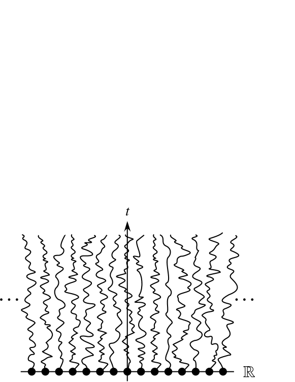
Figure 10: Consider the Dyson model starting from the configuration in which every point of the integers $\mathbb{Z}$ is occupied by one particle. This nonequilibrium determinantal process shows a relaxation phenomenon to the stationary state $\mu_{\sin}$.

As a matter of fact, we have shown that the correlation kernel is given by [45]

$$\mathbb{K}^{\xi^{\mathbb{Z}}}(s,x;t,y)={\bf K}_{\sin}(s,x;t,y)$$

$$\qquad\qquad+\frac{1}{2\pi}\int_{|k|\leq\pi}dk\,e^{k^{2}(t-s)/2+\sqrt{-1}k(y-x)}\Big{\{}\vartheta_{3}(x-\sqrt{-1}ks,2\pi\sqrt{-1}s)-1\Big{\}}$$

$$\qquad={\bf K}_{\sin}(s,x;t,y)$$

$$\qquad\qquad+\sum_{n\in\mathbb{Z}\setminus\{0\}}e^{2\pi\sqrt{-1}xn-2\pi^{2}sn^{2}}\int_{0}^{1}du\,e^{\pi^{2}u^{2}(t-s)/2}\cos\Big{[}\pi u\{(y-x)-2\pi\sqrt{-1}sn\}\Big{]},$$

$(s,t)\in[0,\infty)^{2},(x,y)\in\mathbb{R}^{2}$, where

$${\bf K}_{\sin}(s,x;t,y) = \frac{1}{2\pi}\int_{|k|\leq\pi}dk\,e^{k^{2}(t-s)/2+\sqrt{-1}k(y-x)}-{\bf 1}(s>t)p_{s-t}(x|y)$$ (3.20)

$$= \left\{\begin{array}[]{ll}\displaystyle{\int_{0}^{1}du\,e^{\pi^{2}u^{2}(t-s)/2}\cos\{\pi u(y-x)\}}&\mbox{if $t>s$}\cr&\cr K_{\sin}(x,y)&\mbox{if $t=s$}\cr&\cr\displaystyle{-\int_{1}^{\infty}du\,e^{\pi^{2}u^{2}(t-s)/2}\cos\{\pi u(y-x)\}}&\mbox{if $t<s$},\end{array}\right.$$

with

$$K_{\sin}(x,y)=\frac{1}{2\pi}\int_{|k|\leq\pi}dk\,e^{\sqrt{-1}k(y-x)}=\frac{\sin\{\pi(y-x)\}}{\pi(y-x)},\quad x,y\in\mathbb{R},$$ (3.21)

and $\vartheta_{3}$ is a version of the Jacobi theta function defined by

$$\vartheta_{3}(v,\tau)=\sum_{n\in\mathbb{Z}}e^{2\pi\sqrt{-1}vn+\pi\sqrt{-1}\tau n^{2}},\quad\Im\tau>0.$$ (3.22)

By this explicit expression, we can see that

$$\lim_{u\to\infty}\mathbb{K}^{\xi^{\mathbb{Z}}}(u+s,x;u+t,y)={\bf K}_{\sin}(s,x;t,y).$$ (3.23)

The correlation kernel ${\bf K}_{\sin}(s,x;t,y)$ surviving in the long-term limit is called the extended sine kernel. It is symmetric, ${\bf K}_{\sin}(s,x;t,y)={\bf K}_{\sin}(t,y;s,x)$, and the determinantal process with the correlation kernel ${\bf K}_{\sin}(s,x;t,y)$ is an equilibrium dynamics. It is time-reversal with respect to the determinantal point process $\mu_{\sin}$, in which any spatial correlation function is given by a determinant with the correlation kernel (3.21) called the sine kernel. This stationary state $\mu_{\sin}$ is a scaling limit (called the bulk-scaling-limit) of the eigenvalue distribution of random matrices in GUE [65, 22]. See [83, 70, 67, 43].

The theory of entire functions discusses the relations between the growth of an entire function and the distribution of its zeros [64, 69]. Here we set distributions of zeros as initial configurations satisfying some conditions and control the behavior of particles at infinity to realize nonequilibrium dynamics of long-rang interacting infinite-particle systems. Systematic study of determinantal processes with infinite number of particles exhibiting relaxation phenomena is now in progress [44, 45, 46, 48] .

4 Related Topics

At the end of this manuscript, I briefly introduce related topics, which we are interested in.

4.1 Extreme value distributions of noncolliding diffusion processes

As explained in Section 1.2, BES⁽³⁾ is the conditional BM to stay positive. When we impose an additional condition such that it starts from the origin at time $t=0$ and return to the origin at time $t=1$, the process is called the three-dimensional Bessel bridge with duration 1, which is here denoted by $Y(t),0\leq t\leq 1$.

Here we consider the maximum of $Y(t)$,

$$H_{1}=\max_{0<t<1}Y(t).$$

See Fig.11 We can show that the distribution of $H_{1}$ is described as [52]

$${\rm P}(H_{1}\leq h)=-\frac{1}{2}\sum_{n\in\mathbb{Z}}H_{2}(\sqrt{2}nh)e^{-2h^{2}n^{2}},$$ (4.1)

where $H_{i}(x)$ is the $i$-th Hermite polynomial

$$H_{i}(x)=i!\sum_{j=0}^{[i/2]}\frac{(-1)^{j}(2x)^{i-2j}}{j!(i-2j)!},\quad i\in\{0,1,2,\cdots\}$$ (4.2)

with $[a]$=the greatest integer that is not greater than $a\in\mathbb{R}$. By the equation ${\rm P}(H_{1}\leq h)=\int_{0}^{h}p_{1}(u)du$, the probability density function $p_{1}(u)$ of $H_{1}$ is defined, and $s$-th moment of the random variable $H_{1}$ is calculated by

$${\rm E}[H_{1}^{s}]=\int_{0}^{\infty}dh\,h^{s}p_{1}(s).$$

As discussed by Biane, Pitman, and Yor [2], if we set ${\rm E}[H_{1}^{s}]=2(\pi/2)^{s/2}\xi(s)$, the following equality is established,

$$\xi(s) = \frac{1}{2}s(s-1)\pi^{-s/2}\Gamma(s/2)\zeta(s)$$ (4.3)

$$= \frac{1}{2}+\frac{1}{4}s(s-1)\int_{1}^{\infty}du\,(u^{s/2-1}+u^{(1-s)/2-1})(\vartheta_{3}(0,\sqrt{-1}u)-1),$$

where $\Gamma(z)$ is the gamma function, $\zeta(z)$ is the Riemann zeta function,

$$\zeta(z)=\sum_{n=1}^{\infty}\frac{1}{n^{z}},\quad\Re z>1,$$ (4.4)

and $\vartheta_{3}(v,\tau)$ is given by (3.22). See also Chapter 11 in [87].

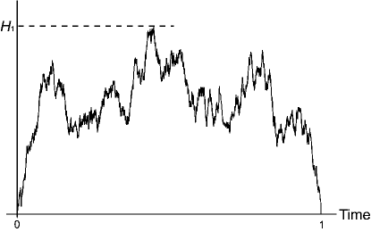
Figure 11: Let $H_{1}$ be the maximum of the three-dimensional Bessel bridge with duration 1. The expectation ${\rm E}[H_{1}^{s}]$ is expressed by using the value of Riemann zeta function at $s\in\mathbb{C}$.

Then we consider an $N$-tuples of three-dimensional Bessel bridges conditioned never to collide with each other, $\mbox{\boldmath$Y$}^{(N)}(t)=(Y^{(N)}_{1}(t),\dots,Y^{(N)}_{N}(t))$,

$$0<Y^{(N)}_{1}<Y^{(N)}_{2}<\cdots<Y^{(N)}_{N},\quad 0<t<1,$$

with $\mbox{\boldmath$Y$}^{(N)}(0)=\mbox{\boldmath$Y$}^{(N)}(1)={\bf 0}$. It is found that (4.1) is generalized for

$$H_{N}=\max_{0<t<1}Y^{(N)}_{N}$$

as [76, 52]

$${\rm P}(H_{N}\leq h)=\frac{(-1)^{N}}{2^{N^{2}}\prod_{i=1}^{N}\Gamma(2i)}\det_{1\leq i,j\leq N}\left[\sum_{n\in\mathbb{Z}}H_{2(i+j-1)}(\sqrt{2}nh)e^{-2n^{2}h^{2}}\right].$$ (4.5)

Extensive study of extreme value distributions of noncolliding processes has been reported in [24, 36, 18, 76, 19, 3, 66, 71, 31]. See also [53, 86, 42, 58].

Recently, Forrester, Majumdar, and Schehr clarified an equality between the distribution function ${\rm P}(H_{N}\leq h)$ and the partition function of the 2$d$ Yang-Mills theory on a sphere with a gauge group ${\rm Sp}(2N)$ [23]. Moreover, by using this equivalence, they proved that in a scaling limit of ${\rm P}(H_{N}\leq h)$, the Tracy-Widom distribution of GOE of random matrices [84, 85] is derived.

4.2 Characteristic polynomials of random matrices

Let ${\cal H}$ be an $N\times N$ Hermitian random matrix in the GUE. The characteristic polynomial of a variable $\alpha$ is then given by

$$P(\alpha)=\det(\alpha I-{\cal H}),$$

where $I$ is the $N\times N$ unit matrix. In the connection with the Riemann zeta function (4.4), statistical property of $P(\alpha)$ has been studied [50, 51, 28, 6]. Here we consider the ensemble average of $m$-product of characteristic polynomials

$$M_{\rm GUE}(m,\mbox{\boldmath$\alpha$};N,\sigma^{2})=\left\langle\prod_{n=1}^{m}P(\alpha_{n})\right\rangle_{{\rm GUE}(N,\sigma^{2})}=\left\langle\prod_{n=1}^{m}\prod_{i=1}^{N}(\alpha_{n}-\lambda_{i})\right\rangle_{{\rm GUE}(N,\sigma^{2})},$$ (4.6)

where $\left\langle\,\cdot\,\right\rangle_{{\rm GUE}(N,\sigma^{2})}$ denotes the ensemble average in the GUE with variance $\sigma^{2}$ of $N\times N$ Hermitian matrices $\{{\cal H}\}$, whose eigenvalues are $\{(\lambda_{i})_{i=1}^{N}\}$. The probability density function of eigenvalues of ${{\cal H}}$ in GUE with variance $\sigma^{2}$ is given by

$$\mu_{N,\sigma^{2}}(\xi)=\frac{\sigma^{-N^{2}}}{C_{N}}\exp\left(-\frac{|\mbox{\boldmath$x$}|^{2}}{2\sigma^{2}}\right)h_{N}(\mbox{\boldmath$x$})^{2},$$ (4.7)

$\xi=\sum_{i=1}^{N}\delta_{x_{i}}\in\mathfrak{M},x_{1}\leq x_{2}\leq\cdots\leq x_{N}$, where $C_{N}=(2\pi)^{N/2}\prod_{i=1}^{N}\Gamma(i)$, $|\mbox{\boldmath$x$}|^{2}=\sum_{i=1}^{N}x_{i}^{2}$, and $h_{N}(\mbox{\boldmath$x$})$ is given by (2.7). Then if the expectation of a measurable function $F$ of a random variable $\Xi\in\mathfrak{M}$ with respect to (4.7) is written as

$${\bf E}_{N,\sigma^{2}}[F(\Xi)]=\int_{\mathbb{W}_{N}^{\rm A}}F(\xi)\mu_{N,\sigma^{2}}(\xi)d\mbox{\boldmath$x$}$$

with setting $\xi=\sum_{i=1}^{N}\delta_{x_{i}},\mbox{\boldmath$x$}=(x_{1},\dots,x_{N})$, where $d\mbox{\boldmath$x$}=\prod_{i=1}^{N}dx_{i}$, (4.6) is written as

$$M_{\rm GUE}(m,\mbox{\boldmath$\alpha$};N,\sigma^{2})={\bf E}_{N,\sigma^{2}}\left[\prod_{n=1}^{m}\prod_{X\in\Xi}(\alpha_{n}-X)\right].$$

In Section 3.3, we showed that the Dyson model $(\Xi(t),\mathbb{P}^{\xi})$ is a determinantal process with the correlation kernel (3.12) for any fixed initial configuration $\xi\in\mathfrak{M}_{0}$ if $\xi(\mathbb{R})=N\in\mathbb{N}$. Here we consider the situation such that the initial configuration $\xi$ is distributed according to (4.7). Note that by the term $h_{N}(\mbox{\boldmath$x$})^{2}$ in (4.7), the GUE eigenvalue distribution is in $\mathfrak{M}_{0}$ w.p.1.

By using Aspect 2 of the Dyson model, we can prove that this process, denoted by $(\Xi(t),\mathbb{P}^{\mu_{N,\sigma^{2}}})$, is equivalent with the time shift $t\to t+\sigma^{2}$ of the Dyson model starting from the configuration $N\delta_{0}$ (i.e., all $N$ particles are put at the origin). That is, the equality

$$(\Xi(t),\mathbb{P}^{\mu_{N,\sigma^{2}}})=(\Xi(t+\sigma^{2}),\mathbb{P}^{N\delta_{0}})$$ (4.8)

holds for arbitrary $\sigma^{2}>0$ in the sense of finite dimensional distribution [35].

This equivalence is highly nontrivial, since even from its special consequence, the following determinantal expression is derived for the ensemble average of product of characteristic polynomials; For any $N,n\in\mathbb{N}$, $\mbox{\boldmath$\alpha$}=(\alpha_{1},\alpha_{2},\cdots,\alpha_{2n})\in\mathbb{C}^{2n}$, $\sigma^{2}>0$,

$$M_{\rm GUE}(2n,\mbox{\boldmath$\alpha$};N,\sigma^{2})=\frac{\gamma_{N,2n}\sigma^{n(2N+n)}}{h_{n}(\alpha_{1},\cdots,\alpha_{n})h_{n}(\alpha_{n+1},\cdots,\alpha_{2n})}$$

$$\quad\times\det_{1\leq i,j\leq n}\left[\frac{1}{\alpha_{i}-\alpha_{n+j}}\left|\begin{array}[]{cc}H_{N+n}(\alpha_{i}/\sqrt{2\sigma^{2}})&H_{N+n}(\alpha_{n+j}/\sqrt{2\sigma^{2}})\cr H_{N+n-1}(\alpha_{i}/\sqrt{2\sigma^{2}})&H_{N+n-1}(\alpha_{n+j}/\sqrt{2\sigma^{2}})\end{array}\right|\right],$$ (4.11)

where

$$\gamma_{N,2n}=2^{-n(2N+2n-1)/2}\prod_{i=2}^{n}\frac{(N+n-i)!}{(N+n-1)!},$$

and $H_{i}(x)$ is the $i$-th Hermite polynomial given by (4.2).

Moreover, in order to simplify the above expression, we can use the following identity, which was recently given by Ishikawa et al. [29] as a generalization of the Cauchy determinant

$$\det_{1\leq i,j\leq n}\left(\frac{1}{x_{i}+y_{j}}\right)=\frac{h_{n}(\mbox{\boldmath$x$})h_{n}(\mbox{\boldmath$y$})}{\prod_{i=1}^{n}\prod_{j=1}^{n}(x_{i}+y_{j})}.$$

For $n\geq 2,\mbox{\boldmath$x$}=(x_{1},\dots,x_{n}),\mbox{\boldmath$y$}=(y_{1},\dots,y_{n}),\mbox{\boldmath$a$}=(a_{1},\dots,a_{n}),\mbox{\boldmath$b$}=(b_{1},\dots,b_{n})\in\mathbb{C}^{n}$,

$$\det_{1\leq i,j\leq n}\left[\frac{1}{y_{j}-x_{i}}\left|\begin{array}[]{cc}1&a_{i}\cr 1&b_{j}\end{array}\right|\right]$$ (4.14)

$$= \frac{(-1)^{n(n-1)/2}}{\prod_{i=1}^{n}\prod_{j=1}^{n}(y_{j}-x_{i})}\left|\begin{array}[]{cccccccc}1&x_{1}&\cdots&x_{1}^{n-1}&a_{1}&a_{1}x_{1}&\cdots a_{1}x_{1}^{n-1}\cr 1&x_{2}&\cdots&x_{2}^{n-1}&a_{2}&a_{2}x_{2}&\cdots a_{2}x_{2}^{n-1}\cr&&\cdots&&&&\cdots\cr 1&x_{n}&\cdots&x_{n}^{n-1}&a_{n}&a_{n}x_{n}&\cdots a_{n}x_{n}^{n-1}\cr 1&y_{1}&\cdots&y_{1}^{n-1}&b_{1}&b_{1}y_{1}&\cdots b_{1}y_{1}^{n-1}\cr 1&y_{2}&\cdots&y_{2}^{n-1}&b_{2}&b_{2}y_{2}&\cdots b_{2}y_{2}^{n-1}\cr&&\cdots&&&&\cdots\cr 1&y_{n}&\cdots&y_{n}^{n-1}&b_{n}&b_{n}y_{n}&\cdots b_{n}y_{n}^{n-1}\cr\end{array}\right|.$$ (4.23)

Then we have the expression

$$M_{\rm GUE}(2n,\mbox{\boldmath$\alpha$};N,\sigma^{2})=\frac{1}{h_{2n}(\mbox{\boldmath$\alpha$})}\det_{1\leq i,j\leq 2n}\left[\widehat{H}_{N+i-1}(\alpha_{j};\sigma^{2})\right],$$ (4.24)

where

$$\widehat{H}_{i}(\alpha;\sigma^{2})\equiv\left(\frac{\sigma^{2}}{2}\right)^{i/2}H_{i}\left(\frac{\alpha}{\sqrt{2\sigma^{2}}}\right).$$

This determinantal expression (4.24) is also obtained from the general formula given by Brézin and Hikami as Eq.(14) in [6]. See [13] for recent development of this topic.

4.3 Fomin’s determinant for loop-erased random walks and its scaling limit

We consider a network $\Gamma=(V,E,W)$, where $V=\{v_{i}\}$ and $E=\{e_{i}\}$ are sets of vertices and of edges of an undirected planar lattice, respectively, and $W=\{w(e)\}_{e\in E}$ is a set of the weight functions of edges. For $a,b\in V$, let $\pi$ be a walk given by

$$\pi\,:\,a=v_{0}\,{\stackrel{{\scriptstyle e_{1}}}{{\rightarrow}}}\,v_{1}\,{\stackrel{{\scriptstyle e_{2}}}{{\rightarrow}}}\,v_{2}\,{\stackrel{{\scriptstyle e_{3}}}{{\rightarrow}}}\,\cdots{\stackrel{{\scriptstyle e_{m}}}{{\rightarrow}}}\,v_{m}=b\,$$

where the length of walk is $|\pi|=m\in\mathbb{N}$ and, for each $0\leq i\leq m-1$, $v_{i}$ and $v_{i+1}$ are nearest-neighboring vertices in $V$ and $e_{i}\in E$ is the edge connecting these two vertices. The weight of $\pi$ is given by $w(\pi)=\prod_{i=1}^{m}w(e_{i})$. For any two vertices of $a,b\in V$, the Green’s function of walks $\{\pi:a\rightarrow b\}$ is defined by

$$W(a,b)=\sum_{m}\sum_{\pi:a\rightarrow b,|\pi|=m}w(\pi).$$

The matrix $W=(W(a,b))_{a,b\in V}$ is called the walk matrix of the network $\Gamma$.

The loop-erased part of $\pi$, denoted by ${\rm LE}(\pi)$, is defined recursively as follows. If $\pi$ does not have self-intersections, that is, all vertices $v_{i},0\leq i\leq m$ are distinct, then ${\rm LE}(\pi)=\pi$. Otherwise, set ${\rm LE}(\pi)={\rm LE}(\pi^{\prime})$, where $\pi^{\prime}$ is obtained by removing the first loop it makes. The loop-erasing operator ${\rm LE}$ maps arbitrary walks to self-avoiding walks (SAWs). Note that the map is many-to-one. For each SAW, $\zeta$, the weight $\widetilde{w}(\zeta)$ is given by

$$\widetilde{w}(\zeta)=\sum_{\pi:{\rm LE}(\pi)=\zeta}w(\pi).$$ (4.25)

We consider the statistical ensemble of SAWs with the weight (4.25) and call it loop-erased random walks (LERWs) [61].

Assume that $A=\{a_{1},a_{2},\dots,a_{N}\}\subset V$ and $B=\{b_{1},b_{2},\dots,b_{N}\}\subset V$ are chosen so that any walk from $a_{i}$ to $b_{j}$ intersects any walk from $a_{i^{\prime}},i^{\prime}>i$, to $b_{j^{\prime}},j^{\prime}<j$. The weight of $N$-tuples of independent walks $a_{1}\,{\stackrel{{\scriptstyle\pi_{1}}}{{\rightarrow}}}\,b_{1},\dots,a_{N}\,{\stackrel{{\scriptstyle\pi_{N}}}{{\rightarrow}}}\,b_{N}$ is given by the product of $N$ weights $\prod_{i=1}^{N}w(\pi_{i})$. Then we consider $N$-tuples of walks $(\pi_{1},\pi_{2},\dots,\pi_{N})$ conditioned so that, for any $1\leq i<j\leq N$, the walk $\pi_{j}$ has no common vertices with the loop-erased part of $\pi_{i}$;

$${\rm LE}(\pi_{i})\cap\pi_{j}=\emptyset,\quad 1\leq i<j\leq N.$$ (4.26)

See Fig.12. By definition, ${\rm LE}(\pi_{j})$ is a part of $\pi_{j}$, and thus nonintersection of any pair of loop-erased parts is concluded from (4.26);

$${\rm LE}(\pi_{i})\cap{\rm LE}(\pi_{j})=\emptyset,\quad 1\leq i<j\leq N.$$

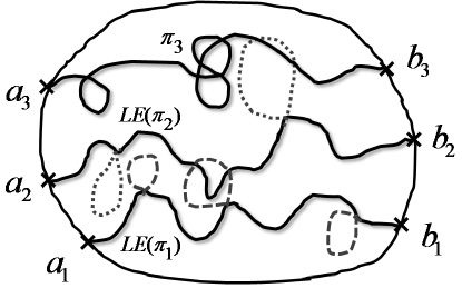
Figure 12: The situation ${\rm LE}(\pi_{j})\cap\pi_{3}=\emptyset,j=1,2$ is illustrated in a planar domain $D$, where $A=(a_{1},a_{2},a_{3})$ and $B=(b_{1},b_{2},b_{3})$ are all boundary points of $\partial D$. In this figure, ${\rm LE}(\pi_{1})$ and ${\rm LE}(\pi_{2})$ denoted by solid curves are the loop-erased parts of the walks $\pi_{1}:a_{1}\rightarrow b_{1}$ and $\pi_{2}:a_{2}\rightarrow b_{2}$, respectively. The third walk $\pi_{3}:a_{3}\rightarrow b_{3}$ can be self-intersecting, but it does not intersect with ${\rm LE}(\pi_{1})$ nor ${\rm LE}(\pi_{2})$.

Fomin proved that total weight of $N$-tuples of walks satisfying such a version of nonintersection condition is given by the minor of walk matrix, $\det(W_{A,B})\equiv\det_{a\in A,b\in B}(W(a,b))$ [21]. This minor is called Fomin’s determinant and Fomin’s formula is expressed by the equality [21, 61]

$$\det(W_{A,B})=\sum_{{\rm LE}(\pi_{i})\cap\pi_{j}=\emptyset,\,i<j}\prod_{k=1}^{N}w(\pi_{k}).$$ (4.27)

Kozdron and Lawler [55] consider continuum limit (the diffusion scaling limit) of Fomin’s determinantal system of loop-erased random walks in the complex plane $\mathbb{C}$, where the initial and the final points $A=\{a_{i}\}$ and $B=\{b_{i}\}$ of paths can be put on the boundaries of the domains $\partial D$. By the diffusion scaling limit each random walk will converge to a path of complex BM. We should note that, however, the characteristics of BM look more similar to those of a surface than those of a curve. It implies that the Brownian path has loops on every scale and then the loop-erasing procedure mentioned above does not make sense for BM in the plane, since we can not decide which loop is the first one. Kozdron and Lawler proved explicitly, however, that the continuum limit of Fomin’s determinant of the Green’s functions of random walks converges to that of the Green’s functions of Brownian motions [55]. This will enable us to discuss nonintersecting systems of loop-erased Brownian paths in the sense of Fomin (4.26). Moreover, Kozdron [54] showed that $2\times 2$ Fomin’s determinant representing the event ${\rm LE}(\beta_{1})\cap\beta_{2}=\emptyset$ for two complex Brownian paths $(\beta_{1},\beta_{2})$ is proportional to the probability that $\gamma_{{\rm SLE}^{(3)}}\cap\beta=\emptyset$, where $\gamma_{{\rm SLE}^{(3)}}$ and $\beta$ denote the SLE⁽³⁾ path and a complex Brownian path, respectively. On the other hand, Lawler and Werner gave a correct way to add ‘Brownian loops’ to an SLE⁽³⁾ path to obtain a complex Brownian path [63]. These results imply that the scaling limit of loop-erased part of complex Brownian path is described by the SLE⁽³⁾ path, as announced in Section 1.4.

Setting a sequence of chambers in a planar domain, Sato and the present author observe the first passage points at which $N$-tuples of complex Brownian paths $(\beta_{1},\dots,\beta_{N})$ first enter each chamber, under the condition that the loop-erased parts $({\rm LE}(\beta_{1}),\dots,{\rm LE}(\beta_{N}))$ make a nonintersecting system in the domain in the sense of Fomin (4.26) [75]. It is proved that the system of first passage points is a determinantal point process in the planar domain, in which the correlation kernel is of Eynard-Mehta type [75]. Interpretation of this result in terms of ‘mutually avoiding SLE paths’ [56, 15] will be an interesting future problem.

Acknowledgements  The present author expresses his gratitude for Jun-ichi Matsuzawa for giving him such an opportunity to give a talk at the Oka symposium. This manuscript is based on the joint work with Hideki Tanemura, Taro Nagao, Naoki Kobayashi, Naoaki Komatsuda, Minami Izumi, and Makiko Sato.

References

- [1] Beffara, V.: The dimension of the SLE curves. Ann. Probab. 36, 1421-1452 (2008)
- [2] Biane, P., Pitman, J., Yor, M.: Probability laws related to the Jacobi theta and Riemann zeta functions, and Brownian excursions. Bull. Amer. Math. Soc. 38, 435–465 (2001)
- [3] Borodin, A., Ferrari, P.L., Prähofer, M., Sasamoto, T., Warren, J.: Maximum of Dyson Brownian motion and non-colliding systems with a boundary. Elect. Commun. in Probab. 14, 486-494 (2009)
- [4] Borodin, A., Rains, E. M.: Eynard-Mehta theorem, Schur process, and their Pfaffian analog. J. Stat. Phys. 121, 291-317 (2005)
- [5] Brézin, E., Hikami, S.: Level spacing of random matrices in an external source. Phys. Rev. E 58, 7176-7185 (1998)
- [6] Brézin, E., Hikami, S.: Characteristic polynomials of random matrices. Commun. Math. Phys. 214, 111-135 (2000)
- [7] Bru, M. F.: Diffusions of perturbed principal component analysis. J. Multivariate Anal. 29, 127-136 (1989)
- [8] Bru, M. F.: Wishart process. J. Theor. Probab. 4, 725-751 (1991)
- [9] Butzer, P. L., Ferreira, P. J. S. G., Higgins, J. R., Saitoh, S., Schmeisser, G., Stens, R. L.: Interpolation and sampling: E. T. Whittaker, K. Ogura and their followers. J Fourier Anal. Appl. (2010) DOI 10.1007/s00041-010-9131-8
- [10] Cardy, J.: Critical percolation in finite geometries. J. Phys. A 25, L201-L206 (1992)
- [11] Cardy, J.: Lectures on conformal invariance and percolation.(2001); arXiv:math-ph/0103018
- [12] Cardy, J., Katori, M.: Families of Vicious Walkers. J. Phys. A 36, 609-629 (2003)
- [13] Delvaux, S.: Average characteristic polynomials in the two-matrix model. (2010); arXiv:math-ph/1009.2447
- [14] Doob, J. L.: Classical Potential Theory and its Probabilistic Counterpart. Springer (1984)
- [15] Dubédat, J.: Euler integrals for commuting SLEs. J. Stat. Phys. 123, 1183-1218 (2006)
- [16] Dyson, F. J.: A Brownian-motion model for the eigenvalues of a random matrix. J. Math. Phys. 3, 1191-1198 (1962)
- [17] Eynard, B., Mehta, M. L.: Matrices coupled in a chain: I. Eigenvalue correlations. J. Phys. A 31, 4449-4456 (1998)
- [18] Feierl, T.: The height of watermelons with wall (extended abstract). Proceedings of the 2007 Conference on Analysis of Algorithms, Discrete Mathematics and Theoretical Computer Science Proceedings, (2007)
- [19] Feierl, T.: The height and range of watermelons without wall (extended abstract). Proceedings of the International Workshop on Combinatorial Algorithms, J. Fiala, J. Kratochvíl, M. Miller (ed), Lecture Notes in Computer Science, Springer, Berlin, vol. 5874, 242-253 (2009)
- [20] Fisher, M. E.: Walks, walls, wetting, and melting, J. Stat. Phys. 34, 667-729 (1984)
- [21] Fomin, S.: Loop-erased walks and total positivity. Trans. Amer. Math. Soc. 353, 3563-3583 (2001)
- [22] Forrester, P. J.: Log-gases and Random Matrices. London Math. Soc. Monographs, Princeton University Press, Princeton (2010)
- [23] Forrester, P. J., Majumdar, S. N., Schehr, G.: Non-intersecting Brownian walkers and Yang-Mills theory on the sphere. Nucl. Phys. B 844 [PM], 500-526 (2011)
- [24] Fulmek, M.: Asymptotics of the average height of 2-watermelons with a wall. Electron. J. Comb. 14, #R64/1–20 (2007)
- [25] Grabiner, D. J.: Brownian motion in a Weyl chamber, non-colliding particles, and random matrices. Ann. Inst. Henri Poincaré, Probab. Stat. 35, 177-204 (1999)
- [26] Harish-Chandra: Differential operators on a semisimple Lie algebra. Am. J. Math. 79, 87-120 (1957)
- [27] Hough, J. B., Krishnapur,M., Peres, Y., Virág, B.: Zeros of Gaussian Analytic Functions and Determinantal Point Processes. University Lecture Series, Amer. Math. Soc., Providence, (2009)
- [28] Hughes, C. P., Keating, J. P., O’Connell, N.: Random matrix theory and the derivative of the Riemann zeta function. Proc. R. Soc. A 456, 2611-2627 (2000)
- [29] Ishikawa, M., Okada, S., Tagawa, H., Zeng, J.: Generalizations of Cauchy’s determinant and Schur’s Pfaffian. Adv. in Appl. Math. 36, 251-287 (2006)
- [30] Itzykson, C., J.-B. Zuber, J.-B.: The planar approximation. II. J. Math. Phys. 21, 411-421 (1980)
- [31] Izumi, M., Katori, M.: Extreme value distributions of noncolliding diffusion processes. to be published in RIMS Kokyuroku Bessatsu; arXiv:math.PR/1005.0533
- [32] Johansson, K.: Non-intersecting paths, random tilings and random matrices. Probab. Th. Rel. Fields 123, 225-280 (2002)
- [33] Johansson, K.: Discrete polynuclear growth and determinantal processes. Commun. Math. Phys. 242, 277-329 (2003)
- [34] Karlin, S., McGregor, J.: Coincidence probabilities. Pacific J. Math. 9, 1141-1164 (1959)
- [35] Katori, M.: Characteristic polynomials of random matrices and noncolliding diffusion processes. (2011); arXiv:math.PR/1102.4655
- [36] Katori, M, Izumi, M. and Kobayashi, N.: Two Bessel bridges conditioned never to collide, double Dirichlet series, and Jacobi theta function. J. Stat. Phys. 131, 1067-1083 (2008)
- [37] Katori, M., Nagao, T. Tanemura, H.: Infinite systems of non-colliding Brownian particles. Adv. Stud. in Pure Math. 39, Stochastic Analysis on Large Scale Interacting Systems, pp.283-306, Math. Soc. Japan, Tokyo, (2004); arXiv:math.PR/0301143
- [38] Katori, M., Tanemura, H.: Scaling limit of vicious walks and two-matrix model. Phys. Rev. E 66, 011105/1-12 (2002)
- [39] Katori, M., Tanemura, H.: Functional central limit theorems for vicious walkers, Stoch. Stoch. Rep. 75, 369-390 (2003); arXiv:math.PR/0203286
- [40] Katori, M., Tanemura, H.: Noncolliding Brownian motions and Harish-Chandra formula. Elect. Comm. in Probab. 8, 112-121 (2003)
- [41] Katori, M., Tanemura, H.: Symmetry of matrix-valued stochastic processes and noncolliding diffusion particle systems. J. Math. Phys. 45, 3058-3085 (2004)
- [42] Katori, M., Tanemura, H.: Infinite systems of noncolliding generalized meanders and Riemann-Liouville differintegrals. Probab. Theory Relat. Fields 138, 113-156 (2007)
- [43] Katori, M., Tanemura, H.: Noncolliding Brownian motion and determinantal processes. J. Stat. Phys. 129, 1233-1277 (2007)
- [44] Katori, M., Tanemura, H.: Zeros of Airy function and relaxation process. J. Stat. Phys. 136, 1177-1204 (2009)
- [45] Katori, M., Tanemura, H.: Non-equilibrium dynamics of Dyson’s model with an infinite number of particles. Commun. Math. Phys. 293, 469-497 (2010)
- [46] Katori, M., Tanemura, H.: Noncolliding squared Bessel processes. J. Stat. Phys. 142, 592-615 (2011)
- [47] Katori, M., Tanemura, H.: Noncolliding processes, matrix-valued processes and determinantal processes. to be published in Sugaku Expositions (AMS); arXiv:math.PR/1005.0533
- [48] Katori, M., Tanemura, H.: Complex Brownian motion representation of the Dyson model. (2010); arXiv:math.PR/1008.2821
- [49] Katori, M., Tanemura, H., Nagao, T., Komatsuda, N.: Vicious walk with a wall, noncolliding meanders, chiral and Bogoliubov-de Gennes random matrices. Phys. Rev. E 68, 021112/1-16 (2003)
- [50] Keating, J. P., Snaith, N. C.: Random matrix theory and . Commun. Math. Phys. 214, 57-89 (2000)
- [51] Keating, J. P., Snaith, N. C.: Random matrix theory and -functions at . Commun. Math. Phys. 214, 91-110 (2000)
- [52] Kobayashi, N., Izumi, M. and Katori, M.: Maximum distributions of bridges of noncolliding Brownian paths. Phys. Rev. E 78, 051102/1-15 (2008)
- [53] König, W., O’Connell, N.: Eigenvalues of the Laguerre process as non-colliding squared Bessel process. Elec. Comm. Probab. 6, 107-114 (2001)
- [54] Kozdron, M.J.: The scaling limit of Fomin’s identity for two paths in the plane. C. R. Math. Rep. Acad. Sci. Canada 29, 448 (2009); arXiv:math.PR/0703615
- [55] Kozdron, M. J., Lawler, G. F.: Estimates of random walk exit probabilities and application to loop-erased random walk. Elect. J. Probab. 10, 1442-1467 (2005)
- [56] Kozdron, M. J., Lawler, G. F.: The configurational measure on mutually avoiding SLE paths. In: Universality and Renormalization : From Stochastic Evolution to Renormalization of Quantum Fields, Binder, I., and Kreimer, D. (ed) (Fields Institute Communications, Vol.50), Amer. Math. Soc., Providence, pp.199-224 (2007); arXiv:math.PR/0605159.
- [57] Krattenthaler, C., Guttmann, A. J., Viennot, X. G.: Vicious walkers, friendly walkers and Young tableaux: II. With a wall. J. Phys. A: Math. Phys. 33, 8835-8866 (2000)
- [58] Kuijlaars, A. B., Martínez-Finkelshtein, A., Wielonsky, F.: Non-intersecting squared Bessel paths and multiple orthogonal polynomials for modified Bessel weight. Commun. Math. Phys. 286, 217-275 (2009)
- [59] Lamperti, J. W.: Semi-stable Markov processes. Z. Wahrscheinlichkeit 22, 205-225 (1972)
- [60] Lawler, G. F.: Conformally Invariant Processes in the Plane. Amer. Math. Soc. (2005)
- [61] Lawler, G. F., Limic, V.: Random Walk: A Modern Introduction. Cambridge University Press, Cambridge (2010)
- [62] Lawler, G.F., Schramm, O., Werner, W.: Conformal invariance of planar loop-erased random walks and uniform spanning trees. Ann. Probab. 32, 939-995 (2004)
- [63] Lawler, G. F., Werner, W.: The Brownian loop soup. Probab. Theory Relat. Fields 128, 565-588 (2004)
- [64] Levin, B. Ya.: Lectures on Entire Functions. Translations of Mathematical Monographs, 150, Providence R. I.: Amer. Math. Soc. (1996)
- [65] Mehta, M. L.: Random Matrices, 3rd ed., Elsevier, Amsterdam (2004)
- [66] Nadal, C., Majumdar, S. N.: Nonintersecting Brownian interfaces and Wishart random matrices. Phys. Rev. E 79, 061117/1-23 (2009)
- [67] Nagao, T., Forrester, P.: Multilevel dynamical correlation functions for Dyson’s Brownian motion model of random matrices. Phys. Lett. A247, 42-46 (1998)
- [68] Nagao, T., Katori, M. Tanemura, H.: Dynamical correlations among vicious random walkers. Phys. Lett. A 307, 29-35 (2003)
- [69] Noguchi, J.: Introduction to Complex Analysis. Translations of Mathematical Monographs, 168, Providence R. I.: Amer. Math. Soc. (1998)
- [70] Osada, H. : Dirichlet form approach to infinite-dimensional Wiener processes with singular interactions. Commun. Math. Phys. 176, 117-131 (1996)
- [71] Rambeau. J., Schehr, G.: Extremal statistics of curved growing interfaces in 1+1 dimensions. Europhys. Lett. 91, 60006/1-6 (2010)
- [72] Revuz, D., Yor, M.: Continuous Martingales and Brownian Motion. 3rd ed., Springer, Now York (1998)
- [73] Rogers, L. C. G., Shi, Z.: Interacting Brownian particles and the Wigner law. Probab. Th. Rel. Fields 95, 555-570 (1993)
- [74] Rohde, S., Schramm, O.: Basic properties of SLE. Ann. Math. 161, 883-924 (2005)
- [75] Sato, M., Katori, M.: Determinantal correlations of Brownian paths in the plane with nonintersection condition on their loop-erased parts. to be published in Phys. Rev. E (2011); arXiv:math-ph/1101.3874
- [76] Schehr, G., Majumdar, S. N., Comtet, A. and Randon-Furling, J.: Exact distribution of the maximum height of vicious walkers, Phys. Rev. Lett. 101, 150601/1-4 (2008)
- [77] Schramm, O.: Scaling limits of loop-erased random walks and uniform spanning trees. Israel J. Math. 118, 221-228 (2000)
- [78] Schramm, O., Sheffield, S.: The harmonic explorer and its convergence to SLE(4). Ann. Probab. 33, 2127-2148 (2005)
- [79] Shirai, T., Takahashi, Y.: Random point fields associated with certain Fredholm determinants I: fermion, Poisson and boson point process. J. Funct. Anal. 205, 414-463 (2003)
- [80] Smirnov, S.: Critical percolation in the plane: conformal invariance, Cardy’s formula, scaling limits. C. R. Acad. Sci. Paris, Sér. I Math. 333, 239-244 (2001)
- [81] Smirnov, S.: Conformal invariance in random cluster models. I. Holomorphic fermions in the Ising model. Ann. Math. 172, 1435-1467 (2010)
- [82] Soshnikov, A. : Determinantal random point fields. Russian Math. Surveys 55, 923-975 (2000)
- [83] Spohn, H. : Interacting Brownian particles: a study of Dyson’s model. In: Hydrodynamic Behavior and Interacting Particle Systems, G. Papanicolaou (ed), IMA Volumes in Mathematics and its Applications, 9, pp. 151-179, Springer, Berlin (1987)
- [84] Tracy, C. A., Widom. H.: Level-spacing distributions and the Airy kernel. Commun. Math. Phys. 159, 151-174 (1994)
- [85] Tracy, C.A., Widom. H.: On orthogonal and symplectic matrix ensembles. Commun. Math. Phys. 177, 727-754 (1996)
- [86] Tracy, C. A., Widom, H. : Nonintersecting Brownian excursions. Ann. Appl. Probab. 17, 953–979 (2007)
- [87] Yor, M.: Some Aspects of Brownian Motion, Part II: Some Recent Martingale Problems. Birkhäuser, Basel (1997)
- [88] Yor, M.: Exponential Functionals of Brownian Motion and Related Processes. Springer (2001)