Polydispersity induced solid-solid transitions in model colloids

Abstract

Specialized Monte Carlo simulation techniques and moment free energy method calculations, capable of treating fractionation exactly, are deployed to study the crystalline phase behaviour of an assembly of spherical particles described by a top-hat “parent” distribution of particle sizes. An increase in either the overall density or the degree of polydispersity is shown to generate a succession of phase transitions in which the system demixes into an ever greater number of face-centred cubic “daughter” phases. Each of these phases is strongly fractionated: it contains a much narrower distribution of particle sizes than is present in the system overall. Certain of the demixing transitions are found to be nearly continuous, accompanied by fluctuations in local particle size correlated over many lattice spacings. We explore possible factors controlling the stability of the phases and the character of the demixing transitions.

I Introduction

Hard spherical particles can be packed to fill maximally just over $74\%$ of space, in the face centred cubic (fcc) structure Hales and Ferguson (2006). For systems in thermal equilibrium such as a colloidal suspension, this structure remains preferred  Woodcock (1997); Bruce et al. (1997) for packing fractions down to about $55\%$ Alder and Wainwright (1957) where melting occurs. But what is the thermodynamically optimal structure for spherical colloids that are “polydisperse”, i.e. have a spread of diameters? Polydispersity should act to destabilize a colloidal crystal because of the difficulty of accommodating a range of particle sizes within a single lattice structure; but despite sustained attention spanning over three decades (see e.g. Dickinson (1978); Barrat, J.L. and Hansen, J.P. (1986); Bartlett (1998); Sear (1998); Phan et al. (1998); Lacks and Wienhoff (1999); Chaudhuri et al. (2005); Fernandez et al. (2007); Yang and Ma (2009)), there is a lack of consensus as to what stable structures arise instead.

Attempts to address this matter have focused on the use of analytical theory and simulation to predict the fate of a single crystal in the dense regime (above typical fluid densities) when the degree of polydispersity becomes large. Broadly speaking, two incompatible proposals have emerged: either the system demixes into multiple coexisting crystalline phases Bartlett (1998); Sear (1998) or, alternatively, crystalline phases disappear altogether Lacks and Wienhoff (1999), the crystal being replaced by an equilibrium glassy phase Chaudhuri et al. (2005). Ideally, of course, one should like to settle the matter as to which (if either) of these scenarios is correct by simply performing an experiment with a suitable suspension of colloids. But the inhibition of diffusion in crystalline phases is expected to render solid-solid demixing transitions largely unobservable on experimental timescales, even if they are thermodynamically favoured. This would – on the face of it – appear to render our central question moot. However, one should recognize that even when equilibrium is itself unattainable in practical situations, independent knowledge of the stable state represents an important baseline for interpreting dynamical properties of colloidal systems (such as crystallization kinetics Auer and Frenkel (2001)) which can be understood in terms of the topology of the free energy surface Poon (2002). There are also suggestions Zaccarelli et al. (2009) that the equilibrium phase diagram sheds light e.g. on the ability of a glassy phase to crystallize. The question as to the nature of the true stable state is thus of more than merely academic interest.

In our view, the disparity in the predictions of previous theoretical and computational work is traceable to the fact that when considering phase separation, little or no account was taken of “fractionation”, i.e. the phenomenon whereby the distribution of the particle diameters, $\sigma$, can vary from one coexisting phase to another Evans et al. (1998); Erne et al. (2005). Indeed it is now well established that fractionation can radically alter the qualitative features of phase behaviour in polydisperse systems compared to their monodisperse counterparts (see Sollich et al. (2001) for a review). Accordingly, it is essential to fully incorporate its effects if one hopes to describe the equilibrium phase behaviour of polydisperse systems correctly Wilding and Sollich (2010).

To quantify fractionation Salacuse and Stell (1982) one simply counts, for a certain phase (labeled $\alpha$), the number density of particles having diameters in the range $\sigma\ldots\sigma+d\sigma$. This serves to define a density distribution $\rho^{(\alpha)}(\sigma)$. However, in real colloidal suspensions, one has the constraint that the overall distribution of sizes (across all phases) has a form fixed by the synthesis of the suspension. This gives rise to a generalized lever rule:

$$\rho^{(0)}(\sigma)=\sum_{\alpha}\lambda^{(\alpha)}\rho^{(\alpha)}(\sigma),$$ (1)

with $\rho^{(0)}(\sigma)$ the “parent” density distribution, $\rho^{(\alpha)}(\sigma)$ the “daughter” distributions, and $\lambda^{(\alpha)}$ the fractional volume occupied by phase $\alpha$ (so that $\sum_{\alpha}\lambda^{(\alpha)}=1$). Since the form of the parent is fixed, only its scale is free to vary, e.g. by dilution with solvent, and one writes $\rho^{(0)}(\sigma)=n^{(0)}f(\sigma)$, where $n^{(0)}$ is the total number density and $f(\sigma)$ is a prescribed normalized shape function. The degree of polydispersity, $\delta$, is then defined as the standard deviation of the parent distribution $f(\sigma)$, expressed in units of its mean.

Fractionation greatly complicates the task of determining the phase behaviour of polydisperse systems compared to their monodisperse counterparts. To illustrate this, consider (for a given colloidal system) increasing $n^{(0)}$ from an initially low value, i.e. following a “dilution line” through the phase diagram of the system. For sufficiently large $n^{(0)}$ the system typically encounters a coexistence region of the phase diagram, which is entered at a “cloud” point Sollich et al. (2001) value of $n^{(0)}$. At and beyond this density the system separates into differently fractionated daughter phases. However, as a consequence of fractionation both the daughter distributions $\rho^{(\alpha)}(\sigma)$ themselves and their associated fractional volumes $\lambda^{(\alpha)}$ depend non-linearly on $n^{(0)}$. Thus in order to quantify the phase behaviour one is faced with the challenge of determining the daughter phase properties for all values of $n^{(0)}$ within the coexistence region – a situation which contrasts with the monodisperse case where the coexistence densities are independent of the total density, whilst the fractional volumes depend linearly on it.

One theoretical technique that does take fractionation into account exactly (within the context of a mean field framework) is the moment free energy (MFE) method. Previous work using this method by one of us Fasolo and Sollich (2004) predicts that, for polydisperse spheres, increasing $\delta$ or $n^{(0)}$ within the solid region leads to a succession of phase transitions in which the system demixes into an ever greater number of differently-fractionated daughter phases. Each daughter phase contains a narrower distribution of particle diameters than the parent. This MFE calculation thus provides clear evidence for the scenario of multiple coexisting solids. But it uses approximate free energy expressions, which for solids are derived from those of binary mixtures and implicitly already assume that all solids are fcc. Independent confirmation of its predictions is then highly desirable, but has hitherto been lacking. The purpose of the present report is therefore to provide a definite answer to the question of the nature of the equilibrium phase behaviour via state-of-the-art Monte Carlo (MC) simulations, and to compare with MFE calculations; both fully provide for fractionation and employ a fixed parent size distribution.

Our paper is organized as follows. In Sec. II we introduce our model systems: size disperse hard spheres (which we have studied by the MFE method), and soft spheres (which we have studied by MC simulation). Sec. III provides a brief description of both the MFE method and the bespoke MC techniques required for dealing with fixed polydispersity and fractionation. Thereafter, in Sec. IV, we report our observations concerning the phase behaviour of these models, the central finding being that the original MFE calculations are indeed correct: as $\delta$ and/or $n^{(0)}$ are increased, a succession of transitions occurs in which the system demixes into first two, then three, then four fractionated coexisting fcc crystalline phases. We analyse the observations to arrive at a qualitative picture of when a crystalline phase will become unstable to phase separation. In Sec. V, we investigate in detail the character of these phase transitions, finding that some are strongly first order, whilst others are quasi-continuous. To quantify the differences, we introduce and measure a susceptibility that probes particle size fluctuations. The associated correlation length at the near continuous transitions is found to extend over several crystal lattice spacings. Prompted by these observations, we use MFE calculations to study in detail how the shape of the size distribution affects the tendency of a given solid phase to exhibit a near continuous demixing transition. This leads us to a simple approximate criterion that quantifies this tendency. Finally, in Sec. VI we summarize and discuss the significance of our results, and indicate some issues for future work.

II Models

The systems that we shall consider in this work are assemblies of spheres interacting either by a repulsive soft sphere potential (as considered by simulation) or a hard sphere potential (as studied in our MFE calculations). The soft sphere interaction potential between two particles $i$ and $j$ with position vectors $\bm{r}_{i}$ and $\bm{r}_{j}$ and diameters $\sigma_{i}$ and $\sigma_{j}$ is given by

$$v(r_{ij})=\epsilon(\sigma_{ij}/r_{ij})^{12}\>,$$ (2)

with particle separation $r_{ij}=|\bm{r}_{i}-\bm{r}_{j}|$ and interaction radius $\sigma_{ij}=(\sigma_{i}+\sigma_{j})/2$. The choice of this potential rather than hard spheres is made on pragmatic grounds; in our isobaric SGCE simulations (to be reported below), any MC contraction of the simulation box that leads to an infinitesimal overlap of two hard spheres would always be rejected, so (particularly at high densities) we can expect higher MC acceptance rates using a “softer” potential. In common with hard spheres, the monodisperse version of our model freezes into an fcc crystalline structure Hansen (1970); Hoover et al. (1970); Wilding (2009), and temperature only plays the role of a scale: the thermodynamic state depends not on $n^{(0)}$ and $T$ separately but only on the combination $n^{(0)}(\epsilon/k_{\mathrm{B}}T)^{1/4}$. Phase diagrams for different $T$ then scale exactly onto one another, and we can fix $\epsilon/k_{\mathrm{B}}T=1$.

In all cases we consider parent size distributions of the top-hat form:

$$f(\sigma)=\left\{\begin{array}[]{ll}(2c)^{-1}&\mbox{ if $1-c\leq\sigma/\bar{\sigma}\leq 1+c$}\\ ~{}~{}0&\mbox{ otherwise }\end{array}\right..$$ (3)

Here the width parameter $c$ controls the degree of polydispersity $\delta=c/\sqrt{3}$. In the following we use the mean particle diameter $\bar{\sigma}$ as our unit of length.

III Methodologies

III.1 Analytical calculations: the moment free energy method

Calculating analytically the phase behaviour of polydisperse systems is a challenging problem Sollich (2002). This is because for each of the infinitely many different particle sizes $\sigma$ one has a separate conserved density $\rho(\sigma)$. Effectively one thus has to study the thermodynamics of an infinite mixture, where e.g. from the Gibbs rule there is no upper limit on the number of phases that can occur.

The moment free energy (MFE) method Sollich et al. (2001); Warren (1998); Sollich and Cates (1998); Sollich (2002) is designed to get around this issue by effectively projecting the infinite mixture problem down to that for a finite mixture of “quasi-species”. This is possible when the free energy density has a so-called truncatable form,

$$f=k_{\mathrm{B}}T\int d\sigma\rho(\sigma)\left[\ln(\rho(\sigma))-1\right]+f^{\rm ex}(\{\rho_{i}\})\ ,$$ (4)

where the excess part $f^{\rm ex}$ depends on a finite number of moments of the density distribution,

$$\rho_{i}=\int d\sigma\rho(\sigma)w_{i}(\sigma)\ .$$ (5)

This truncatable structure obtains for a large number of models of mean field type. Importantly for our purposes, it is also found in accurate free energy expressions for polydisperse hard spheres, with the simple weight functions $w_{i}(\sigma)=\sigma^{i}$ ($i=0,1,2,3$). Specifically, we use the free energy developed by Bartlett Bartlett (1997) on the basis of the simulation data of Kranendonk et al. Kranendonk and Frenkel (1991) for binary mixtures. As mentioned above, this effectively presupposes fcc structures for all solids, so that validation e.g. by simulations, as provided in this paper, is important.

The MFE method provides a way of expressing the ideal contribution to the free energy from Eq. (4), which depends on the complete shape of the density distribution, in terms of the moment densities $\rho_{i}$. The result is the moment free energy. The key feature of the method is that if one then treats the quasi-species densities $\rho_{i}$ as if they were densities of ordinary particle species, and calculates phase equilibria accordingly, the results for cloud points are fully exact. Within coexistence regions, the method can be extended by including additional moments Speranza and Sollich (2002). Their weight functions can be chosen adaptively, and using the resulting approximation as an initialization Speranza and Sollich (2003), the exact phase equilibrium conditions can then be solved numerically, even if e.g. three or four daughter phases are present. Overall, the MFE approach is therefore the method of choice for our current investigation. We do not give further details of the numerical implementation here as these are set out in full in Ref. Fasolo and Sollich (2004).

III.2 Simulation: phase behaviour within the isobaric semi-grand canonical ensemble

The appropriate ensemble for determining phase behaviour in dense assemblies of polydisperse particles is the isobaric variant of the semi-grand canonical ensemble (SGCE) Wilding and Sollich (2010). Within this ensemble, the particle number $N$, pressure $p$, temperature $T$, and a distribution of chemical potential differences $\tilde{\mu}(\sigma)$ are all prescribed, while the system volume $V$, the energy, and the form of the instantaneous density distribution $\rho(\sigma)$ all fluctuate Kofke and Glandt (1988). The fluctuations in $\rho(\sigma)$ are linked to the volume fluctuations by the relation $V\int\rho(\sigma)d\sigma=N$. Importantly, they permit the sampling of many realizations of the polydisperse disorder, thus ameliorating finite-size effects. Moreover, in conjunction with volume fluctuations, they facilitate separation into differently fractionated phases. Coexistence of two or more phases is signalled by a multimodal form for the distribution of some order parameter such as the overall number density $n=N/V$ or the volume fraction $\eta$, which for a phase with density distribution $\rho(\sigma)$ can be written as $\eta=\int d\sigma\rho(\sigma)(\pi/6)\sigma^{3}$.

Operationally, the sole difference between the isobaric semi-grand canonical ensemble and the constant-NpT ensemble Frenkel and Smit (2002) is that one implements MC updates that select a particle at random and attempt to change its diameter $\sigma$ to $\sigma^{\prime}$ by a random amount $\sigma^{\prime}-\sigma$ drawn from a zero-mean uniform distribution. This proposal is accepted or rejected with a Metropolis probability controlled by the change in the internal energy and chemical potential Kofke and Glandt (1988):

$$p_{\rm acc}={\rm min}\left[1,\exp{(-\beta[\Delta\Phi+\tilde{\mu}(\sigma)-\tilde{\mu}(\sigma^{\prime})])}\right]\>,$$

where $\Delta\Phi$ is the internal energy change associated with the resizing operation and $\beta=1/(k_{\mathrm{B}}T)$.

For SGCE simulations of a polydisperse system at some given $N$ and $T$, it is necessary to first determine the pressure $p$ and distribution of chemical potential differences $\tilde{\mu}(\sigma)$ such that a suitably defined ensemble-averaged density distribution matches the prescribed parent $\rho^{(0)}(\sigma)=n^{(0)}f(\sigma)$. Unfortunately, this task is complicated by the fact $p$ and $\tilde{\mu}(\sigma)$ are unknown functionals of the parent Wilding (2003). To solve this problem – and hence determine correct coexistence properties – we shall employ a version of a scheme originally proposed in the context of grand canonical ensemble studies of polydisperse phase coexistence Buzzacchi et al. (2006) and later extended to the SGCE Wilding (2009); Wilding and Sollich (2010), the latter implementation of which we now summarize.

The strategy is as follows. For a given choice of $n^{(0)}$ and temperature $T$, one tunes $p$, $\tilde{\mu}(\sigma)$ and the $\lambda^{(\alpha)}$ iteratively within a histogram reweighting (HR) framework Ferrenberg and Swendsen (1989), such as to simultaneously satisfy both a generalized lever rule and equality of the probabilities of occurrence of the phases, i.e.

$$n^{(0)}f(\sigma) = \sum_{\alpha}\lambda^{(\alpha)}\rho^{(\alpha)}(\sigma),$$ (6a)

$${\mathcal{E}} = 0\>,$$ (6b)

with ${\mathcal{E}}$ as defined in Eq. (8) below. In the first of these constraints, Eq. (6a), the ensemble averaged daughter density distributions $\rho^{(\alpha)}(\sigma)$ are assigned by averaging only over configurations belonging to the respective phase, distinguishable via the multimodal character of the order parameter distribution $p(n)$. The deviation of the weighted sum of the daughter distributions $\bar{\rho}(\sigma)\equiv\sum_{\alpha}\lambda^{(\alpha)}\rho^{(\alpha)}(\sigma)$ from the target $n^{(0)}f(\sigma)$ is conveniently quantified by a “cost” value:

$$\Delta\equiv\int\mid\bar{\rho}(\sigma)-n^{(0)}f(\sigma)\mid d\sigma\;.$$ (7)

In the second constraint, Eq. (6b),

$${\mathcal{E}}\equiv\sum_{\alpha}\left(p^{(\alpha)}-\frac{1}{m}\right)^{2}$$ (8)

provides a measure of the extent to which the probability of each phase occuring, $p^{(\alpha)}$, is equal for each of the $m$ coexisting phases. Imposing this equality ensures that finite-size errors in coexistence parameters are exponentially small in the system volume Borgs and Kotecky (1992); Buzzacchi et al. (2006).

The iterative determination of $p,\tilde{\mu}(\sigma)$ and $\lambda^{(\alpha)}$ such as to satisfy Eqs. (6a) and (6b) proceeds thus:

1. Guess initial values of the fractional volumes $\lambda^{(\alpha)}$ corresponding to the chosen value of $n^{(0)}$. Usually if one starts near a cloud point, the fractional volume of the incipient phase will be close to zero.

2. Tune the pressure $p$ (within the HR scheme) such as to minimize $\Delta$.

3. Similarly tune $\tilde{\mu}(\sigma)$ (within the HR scheme) such as to minimize $\Delta$.

4. Measure the corresponding value of ${\mathcal{E}}$.

5. If ${\mathcal{E}}<{\rm tolerance}$, finish, otherwise vary $\lambda^{(\alpha)}$ (within the HR scheme) and repeat from step 2.

In step $3$ the minimization of $\Delta$ with respect to variations in $\tilde{\mu}(\sigma)$ is most readily achieved Wilding and Sollich (2002) using the following simple iterative scheme for $\tilde{\mu}(\sigma)$:

$$\beta\tilde{\mu}_{k+1}(\sigma)=\beta\tilde{\mu}_{k}(\sigma)+a\ln\left(\frac{n^{(0)}f(\sigma)}{\bar{\rho}(\sigma)}\right)\;,$$ (9)

for iteration $k\to k+1$. This update is applied simultaneously to all entries in the histogram of $\tilde{\mu}(\sigma)$, and thereafter the distribution is shifted so that $\tilde{\mu}(\sigma_{0})=0$, where $\sigma_{0}$ is the chosen reference size. The quantity $0<a<1$ appearing in Eq. (9) is a damping factor, the value of which may be tuned to optimize the rate of convergence. Note that (as described in Buzzacchi et al. (2006)) it is important that one minimizes $\Delta$ and ${\mathcal{E}}$ to a very high precision in order to ensure that the finite-size effects are exponentially small in the system size. Typically we iterated until both were less than $10^{-12}$.

The values of $\lambda^{(\alpha)}$ and $p$ resulting from the application of the above procedure are the desired fractional volumes and pressure corresponding to the nominated value of $n^{(0)}$. As mentioned above, daughter phase densities and volume fractions are obtainable by monitoring the multimodal nature of the order parameter distribution $p(n)$, which allows configurational properties to be assigned to a given phase Wilding (2009).

IV Phase diagram and solid stability

We consider first the overall phase diagram of the soft sphere system as studied in our simulations for a system of $N=256$ particles. Fig. 1a shows (empty symbols) the boundaries of the fluid-solid (FS) coexistence region at low densities. These boundaries are the cloud curves coming from the low and high density regimes, respectively, and were previously determined by us using MC phase-switch techniques Wilding and Sollich (2010). Our focus in this paper is on the solid region at higher densities. Here a comprehensive exploration of the ($n^{(0)}$-$\delta$) plane is impractical because of the relatively high computational cost of our specialized simulation technique. But we can understand important qualitative features by following the dashed trajectory included in Fig. 1a . Along this path, we monitored the state of the system via the probability distribution of the fluctuating total number density $p(n)$, which serves as an order parameter for phase changes. Starting from the fcc solid cloud point at $\delta=6.3\%$, we initially increased $n^{(0)}$ in a stepwise fashion (filled circles) to $n^{(0)}=1.45$, and then switched to increasing $\delta$ at constant $n^{(0)}$ as a potentially faster route to demixing. Indeed, at $\delta\approx 8\%$ there was a smooth change in $p(n)$ from single to double peaked; an example of the double peaked form is shown in Fig. 2a. The two associated phases were identified as being fcc solids. As is physically reasonable, the higher density solid (HDS) daughter phase contains a surplus of the smaller particles while the lower density solid (LDS) phase has more of the larger particles; see Fig. 3 below.

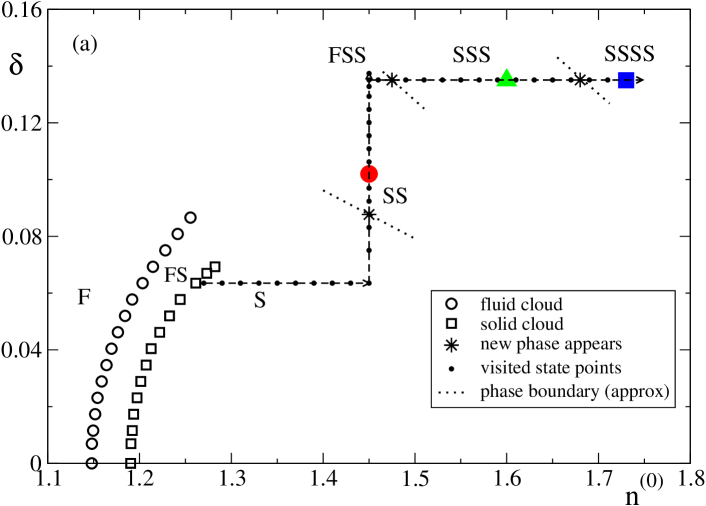
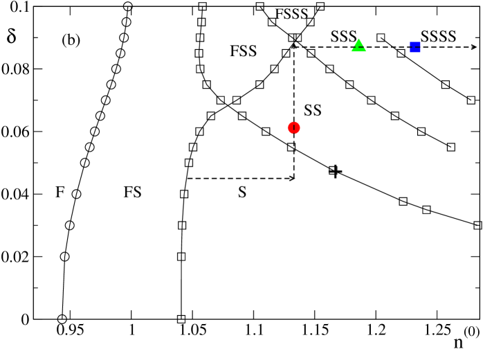
Figure 1: (Color online). (a) Simulation results for the partial phase diagram of the model (2) with parent distribution (3). Asterisks: points where new solid phases appear; dashed lines: phase boundary slopes found by histogram reweighting. F=fluid, S=solid. Colored symbols: state points considered in Fig. 3, 4 and 5. (b) MFE calculation of phase diagram of hard spheres with the same parent form. The dashed line shows a trajectory comparable to that followed by the simulations. The cross marks the critical point for the S–SS transition.

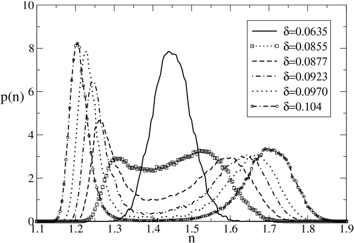
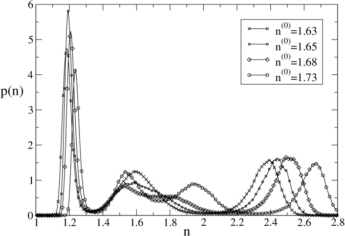
Figure 2: Order parameter distributions through (a, top) the S–SS transition and (b, bottom) the SSS–SSSS transition.

Continuing to higher $\delta$ eventually led to spontaneous melting of the system at $\delta=13.7\%$, implying that the limit of metastability with respect to a fluid-solid-solid (FSS) coexistence had been overstepped, as is indeed predicted by our MFE calculations (see Fig. 1b). We therefore backtracked slightly into the solid-solid (SS) region, embarking on a new trajectory with increasing $n^{(0)}$ at constant $\delta=13.5\%$. This produced a third peak in $p(n)$ at $n^{(0)}\approx 1.475$. The corresponding intermediate density solid (IDS) was again found to be isostructural with the other two, with dominant particle sizes between those in the HDS and LDS. Finally, increasing the overall density to $n^{(0)}\approx 1.68$ we observed that the central IDS peak in $p(n)$ split rather smoothly into two peaks, yielding a four peaked structure (Fig. 2b). All four solids were again identified as having an fcc structure.

We next compare to our theoretical MFE calculations. These used the same parent size distribution (3) but, as explained above, the analysis was performed for hard spheres. The reason is that no suitable polydisperse model free energies are available for the soft repulsive potential (2). Nevertheless, the qualitative physics should be the same. Indeed, taking a comparable path (see Appendix A) through the calculated phase diagram, we find the same features as in the simulations, as shown in Fig. 1b. Quantitatively, the fluid-solid coexistence region is narrower, and transitions to multiple solids occur at lower $n^{(0)}$ and $\delta$, presumably because with a hard repulsion, a crystal can accommodate above average-sized particles less easily.

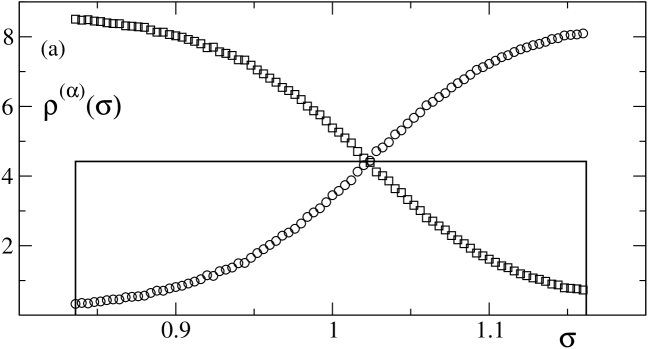
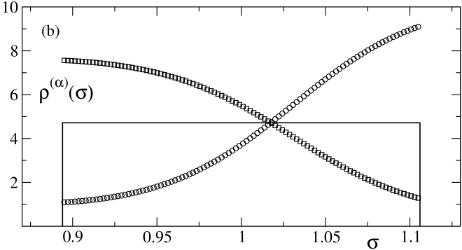
Figure 3: Density distributions in the SS regime. (a) Solid line: Parent density distribution at state point ($n^{(0)}=1.45,\delta=9.5\%$), marked by the red circle in Fig. 1a. Symbols: Simulation results for the two daughter distributions. The associated fractional volumes $\lambda^{(\alpha)}$ are $0.527$ (HDS, squares), $0.473$ (LDS, circles). (b) MFE results at the comparable state point ($n^{(0)}=1.133$, $\delta=6.12\%$), marked by the red circle in Fig. 1b. Fractional volumes are $0.561$ (HDS), $0.439$ (LDS).

A key feature of the phase diagram is the absence of glassy phases. The frustration that could otherwise engender such phases is avoided precisely by fractionation. To illustrate this, we show in Fig. 3 the density distributions for two coexisting solids, at the state points marked by the circles in Fig. 1. The figure also shows the parent density distribution. It is likely that if a single solid were forced to have this size distribution at the density considered, it would indeed assume a disordered, glassy structure. Our results show that at equilibrium, this is avoided by effectively splitting the range of particle sizes among two phases, allowing each phase to remain crystalline on account of its now narrower range of particle size variation. This scenario is then broadly in line with that proposed by Bartlett Bartlett (1998), but the split in sizes is not “sharp” in the sense that particles of a given size would be found exclusively in one phase or the other. Such a sharp split would require infinite differences between phases of the relevant size-dependent chemical potentials. Apart from the general phenomenon of fractionation, Fig. 3 also demonstrates good agreement between the simulation results and the MFE predictions, with e.g. the crossing point between the three density distributions in both cases located somewhat to the right of the parental mean.

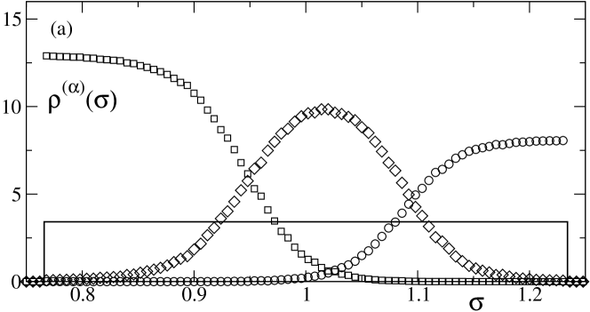
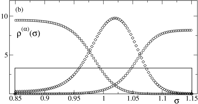
Figure 4: Density distributions in the SSS regime. (a) Solid line: Parent density distribution at state point ($n^{(0)}=1.60,\delta=13.5\%$), marked by the green triangle in Fig. 1a. Symbols: Simulation results for the three daughter distributions. The associated fractional volumes $\lambda^{(\alpha)}$ are $0.267$ (HDS, squares), $0.309$ (IDS, diamonds), $0.424$ (LDS, circles). (b) MFE results at the comparable state point ($n^{(0)}=1.186$, $\delta=8.7\%$), marked by the green triangle in Fig. 1b. Fractional volumes are $0.341$ (HDS), $0.253$ (IDS), $0.405$ (LDS).

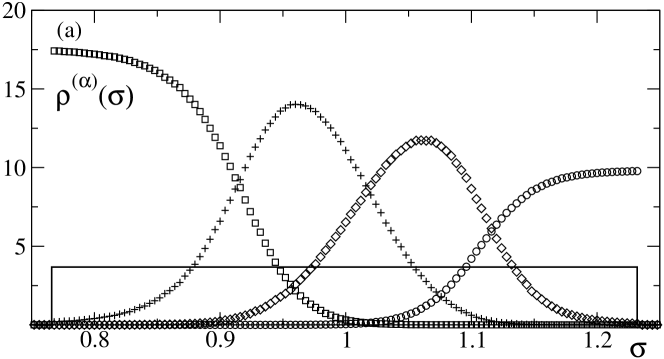
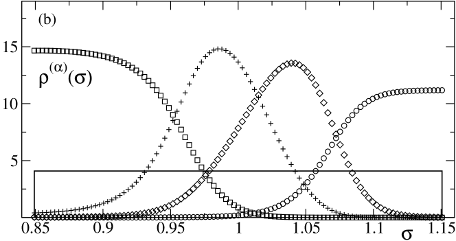
Figure 5: Density distributions in the SSSS regime. (a) Solid line: Parent density distribution at state point ($n^{(0)}=1.73,\delta=13.5\%$), marked by the blue square in Fig. 1a. Symbols: Simulation results for the four daughter distributions. The associated fractional volumes $\lambda^{(\alpha)}$ are, from left to right: 0.209 (HDS, squares), 0.188 (IDS2, $+$), 0.232 (IDS1, diamonds), 0.373 (LDS, circles). (b) MFE results at the comparable state point ($n^{(0)}=1.186$, $\delta=8.7\%$), marked by the blue square in Fig. 1b. Fractional volumes are, from left to right, 0.273, 0.162, 0.200, 0.365. From Ref. Sollich and Wilding (2010). Copyright American Physical Society.

As the density or parent polydispersity of a system in the SS regime are increased further, the polydispersity in the two daughter phases becomes unfavorably large. At this point a third solid appears that takes up the middle of the size distribution, producing three daughters whose size distributions are again sufficiently narrow. This is illustrated in Fig. 4. At the transition from this SSS regime to four solids (SSSS), we then see a process that is qualitatively similar to the S–SS transition: the middle (IDS) phase splits into two phases, each again with a narrower size distribution (Fig. 5). It is worth emphasizing that also in these more complicated fractionation scenarios, the agreement between simulations for soft spheres and theory for hard spheres remains good.

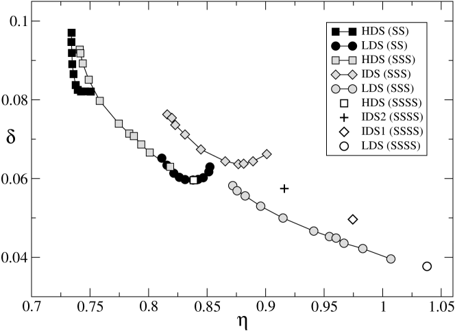
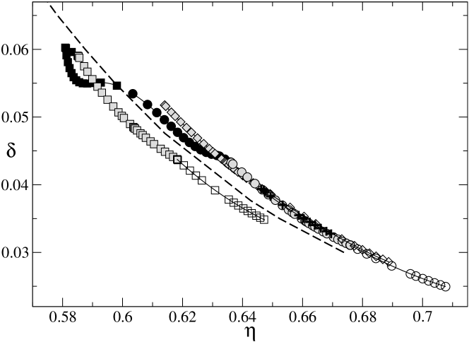
Figure 6: (a, top) Location of daughter phases along the vertical and final horizontal paths in the phase diagram of Fig. 1a, plotted in terms of volume fraction $\eta$ and polydispersity $\delta$. Solid, gray and empty symbols refer to the SS, SSS and SSSS regions, respectively. (b, bottom) Analogous plot for MFE calculations for hard spheres. The additional dashed line indicates the S–SS cloud curve for top hat size distributions from Fig. 1b.

A natural question to ask about the results so far is: what determines the stability of solid phases, i.e. when do new solids appear? Intuitively one would expect that there should be a certain threshold in polydispersity beyond which a given single solid phase would become thermodynamically unfavourable. This threshold should then depend on how dense the phase is: a denser solid can accommodate less variation in particle sizes. To test this idea quantitatively, we plot along the path through our phase diagram the polydispersity $\delta$ versus the volume fraction $\eta$ of all coexisting phases. The results are shown in Fig. 6. One sees that the coexisting phases do indeed cluster around a line in the ($\eta,\delta$) plane, although the clustering is clearly tighter for the MFE (hard sphere) theory. In the plot for the latter case we also show the S–SS phase boundary from Fig. 1b as a dashed line. Recall that this is the boundary as it applies to solids with a top hat size distribution. Most of the coexisting phases that we find lie inside this phase boundary, implying that with their smoother size distributions they can tolerate a somewhat larger amount of polydispersity. In summary, while the general picture of a line in the volume fraction–polydispersity plane where solids become unstable holds true, this line is broadened into a transition region by its dependence on the shape of the size distribution. Motivated by this finding we also experimented with other measures of polydispersity to see whether they would reduce this dependence on distribution shape. In particular, we considered $\delta_{2n}=[\frac{1}{2}\langle(\sigma-\sigma^{\prime})^{2n}\rangle]^{1/(2n)}/\langle\sigma\rangle$ where the averages are over particle sizes $\sigma$ and $\sigma^{\prime}$ randomly drawn from the relevant size distribution. For $n=1$ this gives the conventional $\delta$; for $n\to\infty$ it becomes the difference between the largest and the smallest particle size present, normalized by the mean size. While one may imagine the latter quantity to be the most relevant one for determining crystal stability, we found in practice that the clustering in the ($\eta,\delta_{2n}$) plane becomes worse for larger $n$, with the most easily interpretable results being the ones shown above for $n=1$.

As a final comment on Fig. 6 it is worth highlighting that the phase with the highest density (HDS, shown by squares) in fact always has the smallest volume fraction among the daughter phases for a given parent. This again reflects the strong fractionation effects: as illustrated in Figs. 3–5, the HDS phase contains the smallest particles, and this reduces its volume fraction $\eta$ to the point where it is smaller than for all other phases. This trend is true throughout, i.e. the ordering of the daughter phases by density $n$ is always the reverse of the ordering by volume fraction $\eta$.

V Criticality in transitions to multiple solids

V.1 Order parameter distributions and fractional volumes

In this section we discuss the nature of the transitions as our system of polydisperse spheres fractionates into an increasing number of solids. Our focus will be on the rather surprising finding that these transitions can be nearly continuous in character.

Initial evidence for this claim is provided by Fig. 2 above. This shows the distributions $p(n)$ of the fluctuating number density in the MC simulations, with each peak corresponding to one of the solid phases. One sees in Fig. 2a, for the S–SS transition, that the initial single peak splits smoothly into two nearby peaks which then rapidly move outwards towards more clearly separated densities. This contrasts with what one would have expected for a first order transition, where a new peak appears at some finite distance from the initial peak and gradually acquires more and more weight. Such a scenario is found, along our particular path through the phase diagram, for the SS–SSS transition (data not shown). The SSS–SSSS transition, on the other hand, is again nearly continuous, like the S–SS transition. This can be seen in Fig. 2b, where the middle peak splits smoothly into two new peaks which move apart and form the IDS1 and IDS2 phases.

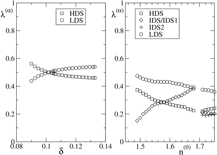
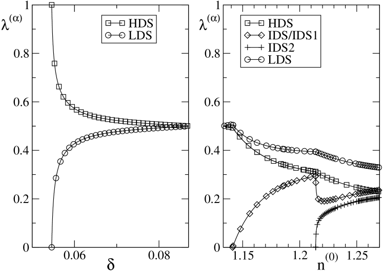
Figure 7: (a, top) Variations of $\lambda$ through transitions from single solid to multiple solids (SS, SSS, SSSS). (b, bottom) Corresponding results from MFE calculations.

Further evidence for nearly continuous transitions to multiple solids is provided by the variation of the fractional phase volumes $\lambda^{(\alpha)}$, shown in Fig. 7. One observes that at the S–SS transition, the fractional volume occupied by the new phase has a strongly nonlinear variation with the parent polydispersity. In fact, looking at the simulation results (Fig. 7a), where we cannot get reliable data close to the transition, one would guess that the fractional volume of the new phase has a discontinuous onset, as is typical of phase transitions which are continuous in the thermodynamic sense. The difficulty in obtaining data close to the transition in simulations stems from the fact that in a finite-sized system the critical density distribution $p(n)$ has two peaks, so that one has to proceed some way into the two phase region before one can be sure that peaks observed in $p(n)$ indicate genuine phase coexistence. Looking at the right half of Fig. 7, the behaviour at the SS–SSS transition is rather different, with the fractional volume taken up by the new phase increasing smoothly from zero in an almost linear fashion. This is in line with expectations for a first order transition. The SSS–SSSS transition, on the other hand, again shows nearly continuous behaviour. As for the S–SS transition, phase coexistence cannot be determined unambiguously from the simulation data for our finite systems, and the data outside of the resulting gap are again suggestive of a jump in the new fractional volume at the transition. The MFE calculations show that there is no real jump, rather a strongly nonlinear increase from zero, so that the transition is close to but not fully critical.

Taken together, the above observations of the behaviour of the density distribution $p(n)$ in the simulations, and of the variation of the fractional phase volumes, provide strong evidence that demixing transitions to multiple solids can be near critical. Along our specific path through the phase diagram, it is the S–SS and SSS–SSSS transitions that are of this type. To investigate this issue in more detail, we now turn to characterizing the near critical properties at the level of single phases, via appropriate correlation functions of particle size fluctuations.

V.2 Correlations in size fluctuations

To define a measure of how strongly spatially correlated size fluctuations are in our solids, we consider first a grand canonical setting for a single phase in a fixed volume $V$, and with imposed chemical potentials $\mu(\sigma)$.

The fluctuating density distribution $\rho(\sigma)$ has ensemble average $\langle\rho(\sigma)\rangle$. If we define moment densities $\rho_{n}=\int d\sigma\rho(\sigma)\sigma^{n}$, then the normalized ensemble average size distribution is $\langle\rho(\sigma)\rangle/\langle\rho_{0}\rangle$. Its variance $\Sigma=\langle\rho_{2}\rangle/\langle\rho_{0}\rangle-(\langle\rho_{1}\rangle/\langle\rho_{0}\rangle)^{2}$ sets the scale for any particle size fluctuations. To define our correlation measure $\chi$, we measure the mean particle size in any configuration, which is $\rho_{1}/\rho_{0}$, and construct its variance across the ensemble. This is then normalized by $\Sigma$ and multiplied by system volume $V$ to get a quantity with the dimension of a volume:

$$\chi=\frac{V\langle\left[\Delta(\rho_{1}/\rho_{0})\right]^{2}\rangle}{\Sigma}$$ (10)

In the thermodynamic limit of large $V$, $\rho_{0}$ and $\rho_{1}$ have small fluctuations so one can expand $\Delta(\rho_{1}/\rho_{0})=(\Delta\rho_{1})/\langle\rho_{0}\rangle-(\Delta\rho_{0})\langle\rho_{1}\rangle/\langle\rho_{0}\rangle^{2}$. Abbreviating the ensemble-averaged mean size as $\bar{\sigma}=\langle\rho_{1}\rangle/\langle\rho_{0}\rangle$, this gives

$$\chi=\frac{V\langle\left[\Delta\rho_{1}-\bar{\sigma}\Delta\rho_{0}\right]^{2}\rangle}{\langle\rho_{0}\rangle^{2}\Sigma}$$ (11)

or in terms of the fluctuating density distribution

$$\chi=\frac{V\langle\left(\int d\sigma(\sigma-\bar{\sigma})\Delta\rho(\sigma)\right)^{2}\rangle}{\langle\rho_{0}\rangle^{2}\Sigma}$$ (12)

The denominator here could also be written as $\langle\rho_{2}\rangle\langle\rho_{0}\rangle-\langle\rho_{1}\rangle^{2}$.

To motivate further the above definition of our measure of correlations $\chi$, one can express it via correlation functions of the full spatially-resolved density $\rho(\bm{r},\sigma)$. The fluctuations of the latter can be expressed in terms of the pair correlation function $g_{\sigma\sigma^{\prime}}(\bm{r})$ between particles of sizes $\sigma$ and $\sigma^{\prime}$ as Hansen and McDonald (1986)

$$\langle\Delta\rho(\bm{r},\sigma)\Delta\rho(\bm{r}^{\prime},\sigma^{\prime})\rangle = \langle\rho(\sigma)\rangle\delta(\bm{r}^{\prime}-\bm{r})\delta(\sigma^{\prime}-\sigma)$$

$${}+\langle\rho(\sigma)\rangle\langle\rho(\sigma^{\prime})\rangle[g_{\sigma\sigma^{\prime}}(\bm{r}^{\prime}-\bm{r})-1]$$

So the numerator of (12) is, using $\Delta\rho(\sigma)=V^{-1}\int d\bm{r}\Delta\rho(\bm{r},\sigma)$,

$$V^{-1}\int\!d\bm{r}\,d\bm{r}^{\prime}d\sigma\,d\sigma^{\prime}(\sigma\!-\!\bar{\sigma})(\sigma^{\prime}\!-\!\bar{\sigma})\langle\Delta\rho(\bm{r},\sigma)\Delta\rho(\bm{r}^{\prime},\sigma^{\prime})\rangle=$$

$$\langle\rho_{0}\rangle\Sigma\!+\!\int\!d\bm{r}\,d\sigma\,d\sigma^{\prime}(\sigma\!\!-\!\!\bar{\sigma})(\sigma^{\prime}\!\!-\!\!\bar{\sigma})\langle\rho(\sigma)\rangle\langle\rho(\sigma^{\prime})\rangle[g_{\sigma\sigma^{\prime}}(\bm{r})\!-\!1]$$

This shows that our definition of $\chi$ is physically reasonable: it is the volume integral of a correlation function that measures the spatial correlations of fluctuations in particle size away from the ensemble mean. We will therefore also refer to $\chi$ as the size fluctuation susceptibility. Note that the trivial first term above makes a contribution of $1/\langle\rho_{0}\rangle$ to $\chi$. This is the unit volume per particle and of order unity in the density range we are considering. We will see below that it is negligible compared to the main contribution from the correlation function integral.

Some care is needed when relating the susceptibility $\chi$ as defined above to a length scale $\xi$ for the spatial correlations of size fluctuations. Away from criticality, and in $d$ spatial dimensions, then since the correlation function being integrated decays on a spatial scale of $\xi$, one estimates $\chi\sim\xi^{d}$. This is the identification we made previously Sollich and Wilding (2010). At criticality, on the other hand, the correlation function appearing above will have a spatial power law decay with $|\bm{r}|^{-d+2-\eta}$ up to the cutoff, and hence the susceptibility scales as $\chi\sim\xi^{2-\eta}$ where $\eta$ is the standard critical exponent (and not, as elsewhere in the paper, the volume fraction).

One can show that, for large systems, the size fluctuations we are considering are the same in all reasonable ensembles, for example a semi-grand canonical ensemble where particle number $N$ is fixed and the volume $V$ can fluctuate. In this case the factor $V$ in (10) is replaced by $N/\langle\rho_{0}\rangle$ to give

$$\chi=\frac{N\langle\left[\Delta(\rho_{1}/\rho_{0})\right]^{2}\rangle}{\langle\rho_{2}\rangle-\langle\rho_{1}\rangle^{2}/\langle\rho_{0}\rangle}$$ (13)

and this is the method we use to extract $\chi$ from simulation data. For the theoretical calculations, we employ (11) and extract the (co-)variances of the fluctuations of the moment densities $\rho_{0}$, $\rho_{1}$ from the appropriate curvature matrix of the moment free energy Sollich et al. (2001).

Note finally that in the context of experiments on colloids a canonical ensemble, with fixed particle number $N$, volume $V$ and parent size distribution, would be the most natural description. For a single phase, the mean size is then fixed and no size fluctuations occur. But $\chi$ can still be defined in terms of the pair correlation function $g_{\sigma\sigma^{\prime}}(\bm{r})$ as described above, provided the spatial integration over $\bm{r}$ is cut off at some distance much larger than the correlation length but much smaller than the system size. This eliminates the contribution from the nonzero values $g_{\sigma\sigma^{\prime}}(\bm{r})-1=O(1/N)$ that remain at larger $\bm{r}$ when the total particle number $N$ is fixed Hansen and McDonald (1986). Once several phases appear, each phase has fluctuating particle numbers and volume, but one can check that the size fluctuations in each phase, and hence the size fluctuation susceptibility, are as would be calculated for single phases in the grand canonical ensemble.

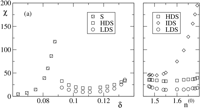
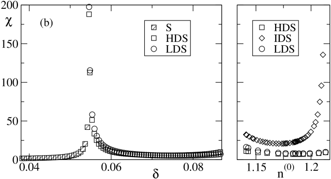
Figure 8: Size fluctuation susceptibility $\chi$ in the solid phases encountered along the phase diagram trajectories of Fig. 1. (a) Simulations, (b) MFE calculations. From Ref. Sollich and Wilding (2010). Copyright American Physical Society.

Having defined how we will quantify the strength of correlations in spatial particle size fluctuations, we show in Fig. 8 results for $\chi$ along the vertical and final horizontal paths through the phase diagrams of Fig. 1. One observes that $\chi$ grows large near the transitions to two and four solids, confirming their near continuous character. In the latter case, the splitting of the middle peak seen earlier in $p(n)$ suggests that the new solids arise out of the IDS phase, and this is consistent with large fluctuations occurring (see Fig. 8) only in this phase and not the HDS or LDS. The MFE predictions are, again, in good qualitative accord with the simulation data.

To summarize our observations in this section, the behaviour of fractional phase volumes and of the order parameter distributions $p(n)$ suggested that phase transitions to multiple solid phases can be near critical in nature; for our path through the phase diagram this applies to the S–SS and SSS–SSSS transitions. We proposed the size fluctuation susceptibility $\chi$ as a quantitative measure of the range of correlations in the spatial fluctuations of particle sizes. Results for this from both simulations and MFE calculations then demonstrated that these transitions are indeed close to critical, being characterized by values of $\chi$ far above the unit volume per particle.

That such critical or near critical transitions from one to several solids might occur is plausible given that S–SS critical points are observed also in simulations of binary hard sphere mixtures Kranendonk and Frenkel (1991). The free energy expression for polydisperse hard spheres that we use in our MFE calculations was devised by Bartlett Bartlett (1997) on the basis of free energies fitted to these binary mixture simulations. The polydisperse system must then “inherit” the existence of critical points, though not in any trivial way. For example, the polydisperse system has many more degrees of freedom for fluctuations in its size distribution, and one can show from this that spinodal densities are always lower in the polydisperse than in the corresponding binary case.

It is worth stressing that even in transitions involving multiple solid phases (SSS–SSSS), criticality is essentially a single-phase property. Indeed, we have found above quite distinct values of $\chi$ in the three coexisting solid phases before the transition to four solids. In the simulations, we have only a single phase in the simulation box for most of the time, which emphasizes further that $\chi$ is determined from the properties of this single phase. To be more precise, there is an effect of the presence of other phases: the lever rule forces the density distributions of all phases to add up to the parent, and this provides constraints on the chemical potentials $\mu(\sigma)$. Once we know these chemical potentials, however, we can determine $\chi$ individually for every phase, independently of the others.

We next ask what features of a given size distribution make it undergo a critical or near critical transition to multiple solids. Having recognized that criticality is a single-phase property, we focus in this enterprise on the cloud point for the transition S–SS from a single solid to two fractionated solids.

V.3 Predicting criticality

The question of determining whether the S–SS transition from a parent with a given size distribution is close to critical can be cast in quantitative terms as follows: how large is the size fluctuation susceptibility $\chi$ at the S–SS cloud point? We investigate this using MFE calculations for the hard sphere case; precise simulation studies would inevitably require finite-size scaling to larger system sizes than we can access using our computational resources.

As explained in Sec. III.1, the free energy expression that we use for polydisperse hard spheres have excess contributions that depend only on the moment densities $\rho_{i}$ with $i=0,1,2,3$, defined by the weight functions $w_{i}(\sigma)=\sigma^{i}$. One can then show in generality (see e.g. Sollich et al. (2001)) that the criterion for a spinodal, where a phase becomes unstable to local density fluctuations, involves these moments as well as those defined by the second-order weight functions $w_{i}(\sigma)w_{j}(\sigma)=\sigma^{i+j}$, giving in our case moments up to $\rho_{6}$. For a given particle size distribution, all the ratios $\rho_{1}/\rho_{0},\ldots,\rho_{6}/\rho_{0}$ are fixed and the density $\rho_{0}\equiv n$ at the spinodal can be found from the spinodal criterion. The additional condition for a spinodal point also to be a critical point involves in addition the third-order weight functions $w_{i}(\sigma)w_{j}(\sigma)w_{k}(\sigma)=\sigma^{i+j+k}$, which produce moments up to $\rho_{9}$. Inserting the spinodal density, the exact critical point condition resulting from our model free energies is then some function of $\rho_{1}/\rho_{0},\ldots,\rho_{9}/\rho_{0}$. These are the 1st to 9th moments of the normalized size distribution, and so whether a parent phase with a given size distribution will exhibit a critical S–SS transition or not depends only on these moments.

Unfortunately, because the solid free energies we use are derived from fits to simulation data Bartlett (1997), the critical point condition that results is far too complicated to allow for any analytical progress. We therefore proceed initially by solving the condition numerically for a range of parent size distributions of interest. The first case to consider is evidently the top hat distribution studied throughout the paper so far. Here there is only a single parameter to vary, namely the polydispersity $\delta$. We solve for each $\delta$ the spinodal condition to find the spinodal density, and then evaluate the critical point condition at this density. It turns out that there is indeed a critical point in the phase diagram, at ($n^{(0)}=1.1669,\delta=0.0472)$. It is marked in Fig. 1b, and lies close to the path through the phase diagram that we have considered above. This rationalizes why the S–SS transition along this path is near critical, with a large value of $\chi$: at the critical point itself, we would have found $\chi$ diverging to infinity at the transition.

The situation with regard to the shape of the parent distribution is not trivial, however. For example, in previous work we considered both triangular and Schulz distributions Fasolo and Sollich (2004), and found no critical points on the S–SS cloud curve in the physically relevant ranges of density and polydispersity. To get more insight, we consider next families of parent distributions where we can tune both the width, as measured by $\delta$, and the shape. Generalizing from the top hat case studied above, we look first at “slanted top hat” parents where the size distribution is $f(\sigma)=A+B\sigma$ in some interval $\sigma_{-}\leq\sigma\leq\sigma_{+}$, and zero otherwise. We adjust $A$, $B$, $\sigma_{-}$ and $\sigma_{+}$ so that $f(\sigma)$ is normalized, has mean 1 as before, and the desired value of $\delta$. This leaves one degree of freedom, which we express via the slant ratio $R=f(\sigma_{+})/f(\sigma_{-})$, with $R=1$ giving back the simple top hat distribution.

Figure 9: Critical polydispersity $\delta$ versus slant ratio $R$ for slanted parents. Dashed: approximation from $s_{v}=0$.

Proceeding as for the top hat parent, we can now determine numerically for fixed slant ratio $R$ the critical value (if any) of $\delta$, or vice versa. In the resulting Fig. 9 we observe that whether or not there are critical points for a given parent shape depends on $R$: for $R$ below around 0.81, no critical points appear; for slightly larger values, two critical points can exist in the phase diagram, and for values of $R$ around unity and above we generically find one critical point.

Figure 10: Size fluctuation susceptibility $\chi$ at S–SS cloud point for slanted parents with density $n^{(0)}=1.133$, versus slant ratio $R$. Bottom inset: $\delta$ at the cloud point. Top inset: Semi-log plot of $\chi$ vs the deviation from the critical slant ratio, $|R-R_{\mathrm{c}}|$. The dashed line is a power law with exponent $-2$.

So far we have asked what marks out parent size distributions that have critical S–SS transitions, which corresponds to $\chi=\infty$ at the cloud point. Here we digress slightly to ask how $\chi$ at the cloud point then varies as we move away from the critical parent shape. Data from MFE calculations are shown for this in Fig. 10, where we consider parents with fixed density $n^{(0)}=1.133$ as on the vertical path in Fig. 1b. For given slant ratio $R$ we find the polydispersity $\delta$ at the cloud point; see the bottom inset of Fig. 10. The main plot displays the resulting cloud point value of the susceptibility $\chi$ against $R$. It is seen to diverge as a critical value $R=R_{\mathrm{c}}$ is approached, and indeed by solving the critical point criterion for the given parent density we find a single such critical value, $R_{\mathrm{c}}=1.734$. This means that if we had considered a parent with this slanted shape, we would have seen – within our MFE calculations for hard spheres – a fully critical S–SS transition on the vertical path in Fig. 1b.

The top inset of Fig. 10 plots the susceptibility $\chi$ versus the distance from the critical parent shape. The data are consistent with a divergence as $\chi\sim|R-R_{\mathrm{c}}|^{-2}$, except for the points nearest $R_{\mathrm{c}}$ either side, where our numerics become unreliable. That exponent value may seem surprising at first: for our mean field free energy, the susceptibility for models in the Ising universality diverges as $\chi\sim|T-T_{\mathrm{c}}|^{-\gamma}$ with $\gamma=1$. But $R$ smoothly changes the parent shape, and the latter is analogous to the Ising magnetization $m$. We should then identify $|R-R_{\mathrm{c}}|$ with $m$ and this leads to the scaling $\chi\sim m^{-\gamma/\beta}\sim|R-R_{\mathrm{c}}|^{-\gamma/\beta}$. For our mean field free energy this gives an exponent value $\gamma/\beta=1/(1/2)=2$, exactly as observed. A more accurate theory which captures the non-mean field Ising singularities would then be expected to give in $d=3$ the exponent $\gamma/\beta=\delta-1\approx 3.9$.

The bottom inset of Fig. 10 shows the value of the polydispersity $\delta$ at the cloud point against the slant ratio $R$, for the same fixed parent density as in the main plot. The variation in $\delta$ is very small, between around 0.052 and 0.056, even though the parent shape changes quite dramatically from $R=1/4$ to $R=4$. This is in line with the expectation that $\delta$ is the main aspect of the size distribution that determines solid stability.

Figure 11: Critical line in the $(a,b)$-plane for Beta size distributions. The density is fixed to $n=1.133$ and the polydispersity $\delta$ is determined from the spinodal condition; it varies very little over the range shown, from 0.0559 to 0.0576. The line resulting from the criterion $s_{v}=0$ is also shown. Both lie significantly below the line for symmetric distributions ($a=b$).

Returning now to the question of what determines whether a given particle size distribution will produce a critical S–SS transition, we broaden our investigation to a wider class of distributions, namely the Beta distributions. These are of the form $f(\sigma)\propto(\sigma-\sigma_{-})^{a}(\sigma_{+}-\sigma)^{b}$ in some interval $\sigma_{-}\leq\sigma\leq\sigma_{+}$, and zero otherwise. The values of the smallest and largest sizes $\sigma_{-}$ and $\sigma_{+}$ and the proportionality coefficient are again adjusted to make $f(\sigma)$ normalized with unit mean and standard deviation $\delta$. The advantage of Beta distributions is that with their two shape parameters, $a$ and $b$, they are more flexible than e.g. the slanted top hat parents from above. In particular, they can interpolate from distributions with fairly sharp cutoffs at the extreme sizes – for low $a$ and $b$, where in particular $a=b=0$ gives back a top hat distribution – to ones with almost Gaussian shape (large $a$ and $b$) where the cutoffs are in the far tails of the distribution.

Figure 12: (a, top) Examples of critical Beta size distributions, corresponding to the values of $(a,b)$ from Fig. 11, with $a=0.5,1,1.5,\ldots,5$ increasing in the direction shown. (b, bottom) Corresponding distributions of $v=\sigma^{3}$, which is proportional to particle volume; these distributions are much more nearly symmetric.

We can now proceed as above and solve the MFE critical point criterion to find out what shape parameters $a$ and $b$ produce critical S–SS transitions. We do this at fixed density, taking again $n^{(0)}=1.133$. The spinodal condition then fixes $\delta$ for given $a$ and $b$, and the critical point gives one additional condition, so that we get a line of critical points in the $a,b$ plane as shown in Fig. 11. What is noticeable is that the critical points lie significantly away from the line $a=b$ where the parent density distribution is symmetric. This is also clearly visible in Fig. 12a, with the critical size distributions having distinct peaks to the right of the mean. One is led to ask whether there are other quantities, related but not identical to particle diameter, that would have more symmetric distributions. An obvious choice is the particle volume, which is proportional to $v=\sigma^{3}$. As Fig. 12b shows, the distributions $f_{v}(v)=f(\sigma)/(3\sigma^{2})$ are indeed much more nearly symmetric at criticality. This suggests that deviations from such symmetry, as measured by the skew

$$s_{v}=\frac{\langle(v-\langle v\rangle)^{3}\rangle}{\langle(v-\langle v\rangle)^{2}\rangle^{3/2}}$$ (14)

indicate deviations from criticality, and conversely $s_{v}=0$ might be a reasonable approximate way of identifying critical size distributions. We have included the line in the $(a,b)$ plane that results when we solve this condition (at the same values of $\delta$ as previously) in Fig. 11. The agreement with the critical line calculated directly from the MFE criticality condition is qualitatively quite good. In particular, the criterion $s_{v}=0$ captures the fact that the critical size distributions are asymmetric when expressed in terms of particle size, with $a>b$ throughout.

Figure 13: Skewness $s_{v}$ of particle volume distribution in the phases occurring along the phase diagram trajectories of Fig. 1. (a, top) Simulation results, (b, bottom) MFE calculations. Comparison with Fig. 8 shows that the near critical phases also have small $s_{v}$.

We have also calculated $s_{v}$ along the path through the phase diagram in Fig. 1 for top hat parents, and show the results in Fig. 13. One observes that the parent phase has relatively low $s_{v}$ at the S–SS transition, in agreement with the large values of the size fluctuation susceptibility $\chi$. Likewise, in the SSS–SSSS transition, the phase that exhibits large $\chi$ and splits in a near critical fashion into two solids also has small $s_{v}$.

Further support for the use of $s_{v}=0$ as an approximate criterion for criticality comes from the fact that $s_{v}$ can be written in terms of moment densities of $\sigma$ as

$$s_{v} = \frac{\langle v^{3}\rangle-3\langle v^{2}\rangle\langle v\rangle+2\langle v\rangle^{3}}{(\langle v^{2}\rangle-\langle v\rangle^{2})^{3/2}}$$ (15)

$$= \frac{\rho_{9}\rho_{0}^{2}-3\rho_{6}\rho_{3}\rho_{0}+2\rho_{3}^{3}}{(\rho_{6}\rho_{0}-\rho_{3}^{2})^{3/2}}$$ (16)

which entails exactly the moment densities $\rho_{0},\ldots,\rho_{9}$ (though not all of them) that we would expect from the general discussion above. Nevertheless the criterion $s_{v}=0$ clearly remains approximate: for the slanted top hat parents, the results in Fig. 9 show that here the agreement with the full criticality criterion is less good. In particular, from $s_{v}=0$ we would predict that there are no critical points for slant ratio $R<1$, whereas in fact critical size distributions exist down to $R\approx 0.81$. The question of whether there is a more accurate yet still simple criterion for S–SS criticality remains open.

VI Discussion and future work

In summary we have deployed tailored Monte Carlo simulation methods and moment free energy calculations to provide conclusive evidence that dense polydisperse spheres at equilibrium demix into coexisting fcc phases, with more phases appearing as the spread of diameters and the number density increase. Up to four coexisting phase were tracked, each of which contained a narrower distribution of particle sizes than is present in the system overall. Interestingly it was observed that for our systems the S–SS and the SSS–SSSS transitions are quasi-critical, characterised by a large correlation length for fluctuations in local particle size. By contrast the SS–SSS transition was found to be strongly first order. To rationalize these observations, we investigated the features of the parental size distribution that control the character of solid demixing transitions. It was found that small skew in the parent distribution of particle volumes ($s_{v}\approx 0$) correlates well with the existence of a quasi-continuous transition, at least for one class of parental distribution shapes.

Whilst our results settle the matter of the true equilibrium behaviour, they leave open the question as to the extent to which this behaviour will be observable in experimental studies of polydisperse systems. Initial indications from recent experiments on colloid-polymer mixtures are that solid-solid demixing does not occur on the timescale of weeks Liddle et al. (2011). Thus the best opportunity to see evidence may be to focus on regions of the phase diagrams where polydisperse solid(s) coexist with a fluid that can transport particles to their preferred solid phase. Additionally it would be interesting to try to manufacture a distribution of particle sizes that has $s_{v}\approx 0$ and then look for an increase in particle size fluctuations in the single solid region, even if the full transition itself is not seen.

As regards the questions that our results pose for further simulation and theoretical work, an interesting matter is that of the fate of the regions of multiple solid coexistence at high volume fraction. As the polydispersity $\delta$ is reduced, it seems clear that all the transition lines to multiple solids (S–SS, SS–SSS, SSS–SSSS etc) must converge on (but never quite reach) the monodisperse close packed limit at $\delta=0,\eta=\pi/\sqrt{18}\approx 74\%$ since the close packed crystal will be unstable to any finite degree of polydispersity. We can also consider what happens if we fix the polydispersity $\delta>0$ and increase the parent volume fraction. The number of fractionated solids will increase without bound as the pressure increases, until at some volume fraction the pressure diverges and the system cannot be compressed further. The locus of these points in the phase diagram forms the infinite pressure line. Also this line must, as $\delta$ is decreased to zero, approach the monodisperse close packed limit $\eta\approx 74\%$.

An intriguing question is whether criticality can play a role in the approach to the close packed limit along the S–SS boundary. As we have seen, it is primarily the parent shape that controls the nature of the S–SS transition. Thus there may exist parent forms for which S–SS demixing is critical at or very near to the close packed limit, and it would be interesting to see whether a simple characterization of such narrow critical parent size distribution forms can be found.

Further solid phases are likely to arise in the phase diagram at values of $\delta$ beyond those that we have explored. For example one could imagine that at very large $\delta$ (for which the system separates into multiple coexisting phases) the smallest particles, rather than forming their own fcc phase, might instead secrete themselves in the interstitials of the fcc solid formed by the largest particles, thus potentially permitting the volume fraction to exceed $74\%$. Indeed this could be a mechanism whereby a unimodal parental distribution might produce familiar substitutionally-ordered phases, such as CsCl, or exotic phases such as AB₂ and AB₁₃ that can appear in binary colloid mixtures Schofield et al. (2005). Investigating this question could – in principle – be tackled by simulation, but is probably beyond the present capabilities of the MFE calculations which are based on free energies that are reliable only for small to moderate $\delta$.

Acknowledgments: Computational results were partly produced on a machine funded by HEFCE’s Strategic Research Infrastructure fund.

Appendix A Comparable locations in soft and hard sphere phase diagrams

It is difficult to map from first principles the simulation phase diagram for soft spheres to the MFE calculations for hard spheres. Existing approaches as summarized in e.g.  Ref. Shumway et al. (1995) do allow one to calculate effective hard sphere diameters for soft particles, but are based on liquid-state correlations and work only up to moderate densities.

We therefore identified comparable points based on the phase diagram topology. In particular, the simulations at polydispersity $\delta=13.7\%$ show an instability towards FSS coexistence very close to the SS–SSS transition (see Fig. 1a). From the density range between these two points, relative to the separation between the SS–SSS and SSS–SSSS transitions, we estimate the corresponding polydispersity for hard spheres to be $\delta=8.7\%$, just below the meeting point of the SS–FSS and SS–SSS lines in Fig. 1b. We find the density corresponding to the vertical trajectory in Fig. 1a ($n^{(0)}=1.45$) similarly: at this density and at $\delta=13.7\%$, the simulations show an SS phase split that is still stable but becomes unstable at slightly higher $\delta$. The corresponding density in the MFE phase can be estimated as $n^{(0)}=1.133$, just below the SS–FSS transition line at $\delta=8.7\%$. This fixes the vertical and final horizontal trajectories through the MFE phase diagram which we use in evaluating e.g. the correlation volume data in Fig. 8.

For the SSSS state point in Fig. 5 we proceed similarly. This point lies on the final horizontal trajectory through the phase diagram, for which we already have the hard sphere polydispersity $\delta=8.7\%$ that corresponds to the simulation value $\delta=13.7\%$. We then estimate the density of the state point so that its density difference to the SSS–SSSS transition, in units of the separation between the SS–SSS and SSS–SSSS transitions, is the same as in the simulations. This gave $n^{(0)}=1.232$. The same method was applied for the SSS state point in Fig. 4. For the SS point in Fig. 3, we simply scaled the polydispersities in proportion to the value of $\delta$ on the horizontal trajectories through the phase diagram, so that $\delta=0.095$ in the simulations is mapped to $\delta=0.095\times 0.087/0.137=0.0612$.

References

- Hales and Ferguson (2006) T. C. Hales and S. P. Ferguson, “A formulation of the kepler conjecture,” Discrete Comput. Geom., 36, 21 (2006), ISSN 0179-5376.
- Woodcock (1997) L. V. Woodcock, “Entropy difference between the face-centred cubic and hexagonal close-packed crystal structures,” Nature, 385, 141 (1997).
- Bruce et al. (1997) A. D. Bruce, N. B. Wilding, and G. J. Ackland, “Free energy of crystalline solids: A lattice-switch monte carlo method,” Phys. Rev. Lett., 79, 3002 (1997).
- Alder and Wainwright (1957) B. J. Alder and T. E. Wainwright, “Phase transition for a hard sphere system,” J. Chem. Phys., 27, 1208 (1957).
- Dickinson (1978) E. Dickinson, “General discussion,” Faraday Discuss. Chem. Soc., 65, 127 (1978).
- Barrat, J.L. and Hansen, J.P. (1986) Barrat, J.L. and Hansen, J.P., “On the stability of polydisperse colloidal crystals,” J. Phys. France, 47, 1547 (1986).
- Bartlett (1998) P. Bartlett, “Fractionated crystallization in a polydisperse mixture of hard spheres,” J. Chem. Phys., 109, 10970 (1998).
- Sear (1998) R. P. Sear, “Phase separation and crystallisation of polydisperse hard spheres,” Europhys. Lett., 44, 531 (1998).
- Phan et al. (1998) S. E. Phan, W. B. Russel, J. Zhu, and P. M. Chaikin, “Effects of polydispersity on hard sphere crystals,” J. Chem. Phys., 108, 9789 (1998).
- Lacks and Wienhoff (1999) D. J. Lacks and J. R. Wienhoff, “Disappearances of energy minima and loss of order in polydisperse colloidal systems,” J. Chem. Phys., 111, 398 (1999).
- Chaudhuri et al. (2005) P. Chaudhuri, S. Karmakar, C. Dasgupta, H. R. Krishnamurthy, and A. K. Sood, “Equilibrium glassy phase in a polydisperse hard-sphere system,” Phys. Rev. Lett., 95, 248301 (2005).
- Fernandez et al. (2007) L. A. Fernandez, V. Martin-Mayor, and P. Verrocchio, “Phase diagram of a polydisperse soft-spheres model for liquids and colloids,” Phys. Rev. Lett., 98, 085702 (2007).
- Yang and Ma (2009) M. Yang and H. Ma, “Solid-solid transition of the size-polydisperse hard sphere system,” J. Chem. Phys., 130, 031103 (2009).
- Note (1) Though see reference Byelov et al. (2010) for a recent experimental observation of solid-solid phase separation in polydisperse platelike particles.
- Auer and Frenkel (2001) S. Auer and D. Frenkel, “Suppression of crystal nucleation in polydisperse colloids due to increase of the surface free energy,” Nature, 413, 711 (2001).
- Poon (2002) W. C. K. Poon, “The physics of a model colloid-polymer mixture,” Journal of Physics: Condensed Matter, 14, R859 (2002).
- Zaccarelli et al. (2009) E. Zaccarelli, C. Valeriani, E. Sanz, W. C. K. Poon, M. E. Cates, and P. N. Pusey, “Crystallization of hard-sphere glasses,” Phys. Rev. Lett., 103, 135704 (2009).
- Evans et al. (1998) R. Evans, D. Fairhurst, and W. Poon, “Universal law of fractionation for slightly polydisperse systems,” Phys. Rev. Lett., 81, 1326 (1998).
- Erne et al. (2005) B. H. Erne, E. van den Pol, G. J. Vroege, T. Visser, and H. H. Wensink, “Size fractionation in a phase-separated colloidal fluid,” Langmuir, 21, 1802 (2005).
- Sollich et al. (2001) P. Sollich, P. B. Warren, and M. E. Cates, “Moment free energies for polydisperse systems,” Adv. Chem. Phys., 116, 265 (2001a).
- Wilding and Sollich (2010) N. B. Wilding and P. Sollich, “Phase behaviour of polydisperse spheres: simulation strategies and an application to the freezing transition,” ArXiv e-prints (2010), arXiv:1008.3068 [cond-mat.soft] .
- Salacuse and Stell (1982) J. J. Salacuse and G. Stell, “Polydisperse systems: Statistical thermodynamics, with applications to several models including hard and permeable spheres,” J. Chem. Phys., 77, 3714 (1982).
- Fasolo and Sollich (2004) M. Fasolo and P. Sollich, “Fractionation effects in phase equilibria of polydisperse hard-sphere colloids,” Phys. Rev. E, 70, 041410 (2004a).
- Hansen (1970) J. P. Hansen, “Phase transition of the Lennard-Jones system. II. high-temperature limit,” Phys. Rev. A, 2, 221 (1970).
- Hoover et al. (1970) W. G. Hoover, M. Ross, K. W. Johnson, D. Henderson, J. A. Barker, and B. C. Brown, “Soft-sphere equation of state,” J. Chem. Phys., 52, 4931 (1970).
- Wilding (2009) N. B. Wilding, “Freezing parameters of soft spheres,” Mol. Phys., 107, 295 (2009a).
- Sollich (2002) P. Sollich, “Predicting phase equilibria in polydisperse systems,” J.Phys: Condensed Matter, 14, R79 (2002).
- Sollich et al. (2001) P. Sollich, P. B. Warren, and M. E. Cates, “Moment free energies for polydisperse systems,” Adv. Chem. Phys., 116, 265 (2001b).
- Warren (1998) P. B. Warren, “Combinatorial entropy and the statistical mechanics of polydispersity,” Phys. Rev. Lett., 80, 1369 (1998).
- Sollich and Cates (1998) P. Sollich and M. E. Cates, “Projected free energies for polydisperse phase equilibria,” Phys. Rev. Lett., 80, 1365 (1998).
- Bartlett (1997) P. Bartlett, “A geometrically-based mean-field theory of polydisperse hard- sphere mixtures,” J. Chem. Phys., 107, 188 (1997).
- Kranendonk and Frenkel (1991) W. G. T. Kranendonk and D. Frenkel, “Computer-simulation of solid liquid coexistence in binary hard- sphere mixtures,” Mol. Phys., 72, 679 (1991).
- Speranza and Sollich (2002) A. Speranza and P. Sollich, “Simplified Onsager theory for isotropic-nematic phase equilibria of length polydisperse hard rods,” J. Chem. Phys., 117, 5421 (2002).
- Speranza and Sollich (2003) A. Speranza and P. Sollich, “Isotropic-nematic phase equilibria of polydisperse hard rods: the effect of fat tails in the length distribution,” J. Chem. Phys., 118, 5213 (2003).
- Kofke and Glandt (1988) D. A. Kofke and E. D. Glandt, Mol. Phys., 64, 1105 (1988).
- Frenkel and Smit (2002) D. Frenkel and B. Smit, Understanding Molecular Simulation (Academic, San Diego, 2002).
- Wilding (2003) N. B. Wilding, “A nonequilibrium Monte Carlo approach to potential refinement in inverse problems,” J. Chem. Phys., 119, 12163 (2003).
- Buzzacchi et al. (2006) M. Buzzacchi, P. Sollich, N. B. Wilding, and M. Müller, “Simulation estimates of cloud points of polydisperse fluids,” Phys. Rev. E, 73, 046110 (2006).
- Wilding (2009) N. B. Wilding, “Solid-liquid coexistence of polydisperse fluids via simulation,” J. Chem. Phys., 130, 104103 (2009b).
- Ferrenberg and Swendsen (1989) A. M. Ferrenberg and R. H. Swendsen, “Optimized Monte-Carlo data-analysis,” Phys. Rev. Lett., 63, 1195 (1989).
- Borgs and Kotecky (1992) C. Borgs and R. Kotecky, “Finite-size effects at asymmetric 1st-order phase-transitions,” Phys. Rev. Lett., 68, 1734 (1992).
- Wilding and Sollich (2002) N. B. Wilding and P. Sollich, “Grand canonical ensemble simulation studies of polydisperse fluids,” J. Chem. Phys., 116, 7116 (2002).
- Note (2) In the analogous diagram of Ref. Sollich and Wilding (2010), the S–SS phase boundary was erroneously drawn slightly too low, at .
- Sollich and Wilding (2010) P. Sollich and N. B. Wilding, “Crystalline phases of polydisperse spheres,” Phys. Rev. Lett., 104, 118302 (2010).
- Hansen and McDonald (1986) J. P. Hansen and I. R. McDonald, Theory of simple liquids (2nd ed.) (Academic Press, London, 1986).
- Fasolo and Sollich (2004) M. Fasolo and P. Sollich, “Fractionation effects in phase equilibria of polydisperse hard-sphere colloids,” Phys. Rev. E, 70, 041410 (2004b).
- Liddle et al. (2011) S. Liddle, , T. Narayanan, and W. Poon, J. Phys. Condens. Matter (2011), doi:10.1021/jp037487t.
- Schofield et al. (2005) A. B. Schofield, P. N. Pusey, and P. Radcliffe, “Stability of the binary colloidal crystals and ,” Phys. Rev. E, 72, 031407 (2005).
- Shumway et al. (1995) S. L. Shumway, A. S. Clarke, and H. Jonsson, “Molecular-dynamics simulations of a pressure-induced glass- transition,” J. Chem. Phys., 102, 1796 (1995).
- Byelov et al. (2010) D. V. Byelov, M. C. D. Mourad, I. Snigireva, A. Snigirev, A. V. Petukhov, and H. N. W. Lekkerkerker, “Experimental observation of fractionated crystallization in polydisperse platelike colloids,” Langmuir, 26, 6898 (2010).