Gamma-ray bursts afterglows in magnetized stellar winds

Abstract

Recent analytical and numerical work argue that successful relativistic Fermi acceleration requires a weak magnetization of the unshocked plasma, all the more so at high Lorentz factors. The present paper tests this conclusion by computing the afterglow of a gamma-ray burst outflow propagating in a magnetized stellar wind using “ab initio” principles regarding the microphysics of relativistic Fermi acceleration. It is shown that in magnetized environments, one expects a drop-out in the X-ray band on sub-day scales as the synchrotron emission of the shock heated electrons exits the frequency band. At later times, Fermi acceleration becomes operative when the blast Lorentz factor drops below a certain critical value, leading to the recovery of the standard afterglow light curve. Interestingly, the observed drop-out bears resemblance with the fast decay found in gamma-ray bursts early X-ray afterglows.

1 Introduction

The prompt emission of gamma-ray bursts (GRB) is followed by an afterglow phase commonly attributed to the synchrotron emission of shock accelerated electrons (Mészáros & Rees 1997). As the blast wave sweeps up matter and decelerates, the dissipated power decreases and the emission shifts to longer wavebands (e.g., Piran 2005). To model this afterglow emission, one usually encodes the acceleration physics in a minimal/maximal Lorentz factor ($\gamma_{\rm min}\,/\,\gamma_{\rm max}$), in the spectral index $s$ of the electron spectrum, in the fraction $\epsilon_{e}$ of the dissipated energy that is carried by these electrons and in the fraction $\epsilon_{B}$ stored in magnetic turbulence.

However, our understanding of relativistic Fermi acceleration has made significant progress in the last decade, to an extent that motivates a direct test against observational data. The convergence of analytical calculations and extensive particle-in-cell (PIC) numerical calculations has led in particular to the following picture. At (superluminal) ultra-relativistic shock waves, Fermi power-laws cannot develop because the particles get advected to the far downstream along with the magnetic field lines to which they are tied (Begelman & Kirk 1990), unless strong turbulence has been excited on scales significantly smaller than their Larmor radius (Lemoine et al. 2006; Niemiec et al. 2006; Pelletier et al. 2009). In very weakly magnetized shocks, such turbulence can be excited by micro-instabilities in the shock precursor and therefore Fermi acceleration can develop, as confirmed by recent PIC simulations (Sironi & Spitkovsky 2011). The critical level of magnetization below which this turbulence develops depends on the shock Lorentz factor (Lemoine & Pelletier 2010, 2011) as indeed, such instabilities can grow only if their growth timescale is shorter than the timescale on which the unshocked plasma crosses the shock precursor and, the stronger the upstream background magnetization, or the larger the shock Lorentz factor, the shorter the precursor.

In practice, one may expect Fermi acceleration to proceed unhampered if the blast wave propagates in a weakly magnetized external medium such as the interstellar medium (ISM). In magnetized stellar winds, however, one might expect to see signatures of the above microphysics of Fermi acceleration, all the more so at early stages when the blast Lorentz factor is large. Such signatures would open a window on the physics of collisionless relativistic shocks as well as on the astrophysics of GRB afterglows. This motivates the present study, which proposes to compute the afterglow light curve of a gamma-ray burst propagating in a magnetized stellar wind from “ab initio” principles regarding Fermi acceleration.

The recent studies of Li & Waxman (2006) and Li (2010) offer an interesting perspective on this problem. From the observation of X-ray afterglows on sub-day scales, these authors infer a strong lower bound on the upstream magnetic field of gamma-ray bursts afterglows, $B_{\rm u}\gtrsim 200\,\mu{\rm G}\,n_{\rm 0}^{5/8}$ ($n_{0}$ the upstream density in cm^-3); Li (2010) actually derives a significantly stronger bound by considering on equal grounds the long lived high energy emission $>100\,$MeV. This implies that either micro-instabilities have grown and excited the magnetic field to the above values, or the pre-existing magnetic field itself satisfies this bound. While the former is expected if the circumburst medium is ISM like, the latter corresponds to a magnetized circumburst medium. It is this possibility that will be addressed and tested in the present work.

Section 2 presents an analytical discussion of the model and is followed by numerical calculations of the light curve in Sec. 3. Section 4 discusses the results in the light of modern X-ray afterglows.

2 Physical model

We consider the following fiducial values for the parameters characterizing the afterglow. The ejecta is composed of a homogeneous shell of width $\Delta=cT$ with $T=10T_{1}\,$s in the stationary frame, with (isotropic equivalent) bulk kinetic energy $E=10^{54}\,E_{54}\,$erg and Lorentz factor $\gamma_{\rm ej}=300\gamma_{\rm ej,2.5}$. This outflow impinges on a stellar wind with density profile $\rho_{\rm w}=Ar^{-2}$, with $A=5\times 10^{11}A_{*}\,$g/cm and (toroidal) magnetic field profile $B_{\rm w}=10^{3}B_{*}\,{\rm G}\,\left(r/10^{12}\,{\rm cm}\right)^{-1}$; the variables $A_{*}$ and $B_{*}$ encode our uncertainty on the density and the magnetic field. The value $B_{*}=1$ corresponds to the formation of a magnetar with surface field $\sim 10^{15}\,$G after the collapse of a $10R_{\odot}$ progenitor star. The magnetic field of Wolf-Rayet stars, which are considered as potential progenitor stars for gamma-ray bursts, are not known, but surface values as large as $1-10\times 10^{3}\,$G have been considered (Ignace et al. 1998). For these parameters, the magnetization $\sigma_{\rm w}\equiv B_{\rm w}^{2}/\left(4\pi\rho_{\rm w}c^{2}\right)\simeq 1.8\times 10^{-4}B_{*}^{2}A_{*}^{-1}$; it does not depend on $r$. Note that the central assumption here is that of a relatively high magnetization of the external medium; the density profile does not play a crucial role and similar effects can be observed in a constant density medium of sufficient magnetization, as discussed briefly in Sec. 4.

The proper density of the ejecta $n_{\rm ej}=E_{\rm ej}/\left(4\pi r^{2}\gamma_{\rm ej}^{2}\Delta m_{p}c^{2}\right)$; therefore the density contrast between the ejecta and the external medium is not very large, $\left(n_{\rm ej}/n_{\rm w}\right)^{1/2}\simeq 81T_{1}^{-1/2}\gamma_{\rm ej,2.5}^{-1}E_{54}^{1/2}A_{*}^{-1/2}$, implying that the reverse shock propagates at relativistic speeds in the ejecta (Sari & Piran 1995). The shocked material – which we denote as the blast – thus moves with initial Lorentz factor

$$\gamma_{\rm b}\simeq\frac{\gamma_{\rm ej}^{1/2}}{\sqrt{2}}\left(\frac{n_{\rm ej}}{n_{\rm w}}\right)^{1/4}\simeq 110\,T_{1}^{-1/4}E_{54}^{1/4}A_{*}^{-1/4}\ .$$ (1)

It remains constant as long as the reverse shock is crossing the shell (Sari & Piran 1995, Beloborodov & Uhm 2006). Approximating the velocity of the reverse shock as $c$ in the ejecta frame, the reverse shock has crossed the outflow at radius $r_{\times}=\gamma_{\rm b}^{2}cT$ (in the stationary frame), corresponding to observer time $t_{\times}\simeq 5\,{\rm sec}\,(1+z)T_{1}$, with $z$ the GRB redshift.

Beyond $r_{\times}$, the blast Lorentz factor decreases according to $\gamma_{\rm b}\simeq\gamma_{\rm b,\times}\left(r/r_{\times}\right)^{-1/2}$ in the adiabatic regime, $\gamma_{\rm b,\times}$ corresponding to Eq. (1). The relationship between observer time, radius and blast Lorentz factor then becomes $\left(t_{\rm obs}/t_{\times}\right)\simeq\left(r/r_{\times}\right)^{2}\simeq\left(\gamma_{\rm b}/\gamma_{\rm b,\times}\right)^{-4}$.

We now come to the modelling of the electron population in the blast. Following Lemoine & Pelletier (2010, 2011), we define the parameter $Y_{\rm inst}\equiv\xi_{\rm b}^{-1}\sigma_{\rm w}\gamma_{\rm sh}^{2}$, which characterizes whether instabilities may develop or not in the shock precursor, hence whether Fermi cycles can develop or not. The parameter $\xi_{\rm b}$ denotes the fraction of incoming matter energy through the shock $4\gamma_{\rm b}^{2}\rho_{\rm w}c^{2}$ that is carried by the accelerated and returning particles (i.e. the beam). By returning, it is meant those incoming protons that are reflected on the shock front, which constitute an essential ingredient of the shock formation. These reflected protons exist even in the absence of Fermi powerlaws. Through mixing with the unshocked plasma, these returning particles (along with the accelerated particles) induce two-stream or filamentation micro-instabilities in the shock precursor, on scales close to the electron to ion skin depth $c/\omega_{\rm pe}\rightarrow c/\omega_{\rm pi}$. The filamentation instability has time to grow only if $Y_{\rm inst}\,\ll\,1$, while other two stream instabilities may grow faster but are inhibited once the background electrons are heated to relativistic temperatures in the shock precursor (Lemoine & Pelletier 2011). For this reason, we consider only the growth of the filamentation instability in the following. We define a threshold value $Y_{\rm c}$ such that if $Y_{\rm inst}<Y_{\rm c}$, micro-instabilities can grow and allow Fermi cycles to develop, as discussed further below, while if $Y_{\rm inst}>Y_{\rm c}$, instabilities cannot grow, hence Fermi cycles do not develop.

One must expect $Y_{\rm inst}>Y_{\rm c}$ in the early stages of the afterglow, since

$$Y_{\rm inst}\simeq 43\,B_{*}^{2}A_{*}^{-3/2}T_{1}^{-1/2}E_{54}^{1/2}\xi_{\rm b,-1}^{-1}\left(\frac{r}{r_{\times}}\right)^{\alpha_{Y}}\ ,$$ (2)

with $\alpha_{Y}=0$ for $r<r_{\times}$ and $\alpha_{Y}=-1$ for $r>r_{\times}$. PIC simulations indicate that $\xi_{\rm b,-1}\equiv\xi_{\rm b}/0.1\simeq 1$ (Sironi & Spitkovsky 2011).

Early on, as $Y_{\rm inst}>Y_{\rm c}$, micro-instabilities are quenched by advection of the plasma through the shock front, hence the magnetic field is everywhere transverse to the shock normal without substantial inhomogeneity on short scales. In this case, Fermi acceleration cannot develop as particles are advected with the magnetic field lines to the far downstream. Nevertheless, the electrons acquire part of the kinetic energy of the incoming protons in the shock transition (as viewed in the shock frame). A detailed understanding of this process is still lacking but current PIC simulations confirm the above, even in the absence of filamentation in the precursor. In particular, Sironi & Spitkovsky (2011) observe that $\epsilon_{e}$ reaches the value of $0.1$ at a magnetization $\sigma_{\rm u}=10^{-4}$, for $\gamma_{\rm sh}\simeq 20$ and larger. We adopt this value in the following. For simplicity, we model the shock heated electron distribution as a restricted powerlaw with $\gamma_{\rm max}=3\gamma_{\rm min}$. The minimal Lorentz factor $\gamma_{\rm min}$ is then related to $\epsilon_{e}$ through $\gamma_{\rm min}=\epsilon_{e}\gamma_{\rm b}(m_{p}/m_{e})a_{\rm s}$ with $a_{\rm s}=\left[(s-2)/(s-1)\right]\left[1-(\gamma_{\rm max}/\gamma_{\rm min})^{1-s}\right]\left[1-(\gamma_{\rm max}/\gamma_{\rm min})^{2-s}\right]^{-1}$ a normalization prefactor of order unity, which depends (slightly) on the modelling of the energy distribution; we adopt $s=2.4$, an ad-hoc choice here as well motivated by simplicity (i.e. $s$ will not change once Fermi acceleration becomes effective). Although the electrons are heated in the shock transition, the magnetic field is only compressed, so that the magnetic field in the blast frame $B_{\rm b}=4\gamma_{\rm b}B_{\rm w}$. In terms of the conventional parameter $\epsilon_{B}$ describing the fraction of energy carried by the magnetic field in the blast, $\epsilon_{B}=B_{\rm b}^{2}/(8\pi e_{\rm b})=2\sigma_{\rm w}$.

As the blast Lorentz factors decreases beyond $r_{\times}$, so does $Y_{\rm inst}$, until $Y_{\rm inst}<Y_{\rm c}$ eventually. The filamentation instability now has several to many $e-$folds of growth times before the plasma is advected through the shock front. This has several consequences of importance. First of all, the upstream electrons are heated in the micro-turbulence in the shock precursor (Spitkovsky 2008, Lemoine & Pelletier 2011) and they therefore reach rough equipartition with the incoming protons after the shock transition, as observed in PIC simulations (Sironi & Spitkovsky 2011). This implies $\epsilon_{e}\simeq 0.5$. Furthermore, a micro-turbulent magnetic field is generated on skin depth scales up to $\epsilon_{B}$ of a few percents. We adopt $\epsilon_{B}=0.05$ as a fiducial value in what follows, in the absence of more detailed results from PIC simulations in the parameter range of interest. Finally, as discussed above, the micro-turbulence unlocks the particles off the magnetic field lines and allow them to scatter repeatedly back and forth the shock wave, leading to a power-law extension beyond the (relativistic) thermal population. This fact has been clearly observed in the PIC simulations of Sironi & Spitkovsky (2011), for $\gamma_{\rm sh}\simeq 20$ and upstream magnetization $10^{-5}$ (and mass ratio $m_{p}/m_{e}=16$). Note that the same simulations at magnetization $10^{-4}$ do not observe signs of Fermi acceleration, suggesting that $Y_{\rm c}\lesssim 0.5$. In the following, we keep manifest the dependence on $Y_{\rm c}$. To model the resulting electron distribution, we use a power-law between $\gamma_{\rm min}$ and $\gamma_{\rm max}$, with $\gamma_{\rm min}$ related to $\epsilon_{e}$ as before (although here, $\epsilon_{e}\simeq 0.5$); we keep $s=2.4$. This implies that we do not distinguish between the thermal and the powerlaw tail populations; this is a good approximation, since both radiate in synchrotron, hence the above simplification only affects the flux normalization at high energies.

Synchrotron energy losses provide an upper bound on the maximal Lorentz factor, $\gamma_{\rm max}\,\lesssim\,4\times 10^{6}E_{54}^{1/8}T_{1}^{3/8}A_{*}^{-3/8}\epsilon_{B,-1.3}^{-1/4}(r/r_{\times})^{3/4}$ (at $r>r_{\times}$, with $\epsilon_{B,-1.3}=\epsilon_{B}/0.05$). In the present case, the actual limiting factor for $\gamma_{\rm max}$ comes from the scattering properties of accelerated particles in the micro-turbulence, as discussed in Pelletier et al. (2009). Indeed, Fermi cycles can develop if the angular scattering in the micro-turbulence dominates over the regular Larmor orbits in the background field on a cycle timescale, which requires $r_{\rm L,0}\lesssim\ell_{\rm c}(\delta B/B)^{2}$, with $r_{\rm L,0}$ the Larmor radius in the background field $4\gamma_{\rm b}B_{\rm w}$, $\ell_{\rm c}$ the micro-turbulence scale and $\delta B$ the microturbulence strength. Both simulations (e.g., Sironi & Spitkovsky 2011) and analytical arguments (e.g. Lemoine & Pelletier 2011) indicate that the relevant length scale is the ion skin depth $\delta_{\rm i}$ (as measured in the upstream frame), while $(\delta B/B)^{2}\simeq\epsilon_{B}/\sigma_{\rm w}$. This implies a maximal Lorentz factor

$$\gamma_{\rm max}\,\sim\,9\times 10^{5}E_{54}^{1/4}T_{1}^{-1/4}A_{*}^{1/4}\epsilon_{B,-1.3}B_{*}^{-1}\left(\frac{r}{r_{\times}}\right)^{-1/2}\ ,$$ (3)

assuming here $r>r_{\times}$.

Several remarks are in order at this stage. We do not consider the issue of the evolution of the micro-turbulence in the downstream, which remains an open problem in this field (Gruzinov & Waxman 1999, Medvedev & Loeb 1999). The typical Larmor radius of electrons of Lorentz factor $\gamma_{\rm b}m_{p}/m_{e}\sim\gamma_{\rm min}$ reads $r_{L}\sim\delta_{\rm i}/\epsilon_{B}^{1/2}$, hence the first generations of accelerated electrons only probe the vicinity of the shock front in terms of $\delta_{\rm i}$, where the turbulence should not have evolved strongly. In our case, the electron population develops on a a dynamic range $\sim\delta B/B\sim(\epsilon_{B}/\sigma_{\rm w})^{1/2}\lesssim 10^{2}$, see Eq. (3). Therefore the highest energy electrons explore the blast up to $\sim 10^{4}\delta_{\rm i}$ (given that the scattering length in the micro-turbulence scales as $\gamma_{e}^{2}$); admittedly, one cannot exclude that the turbulence evolves on such length scales. For reference, the ion skin depth $\delta_{\rm i}\simeq 2.8\times 10^{5}\,{\rm cm}\,E_{54}^{1/2}T_{1}^{1/2}A_{*}^{-1}(r/r_{\times})$.

We also neglect the influence of extra large scale sources of turbulence, associated with e.g. instabilities of the blast itself (e.g. Levinson 2010), or with the interactions of the shock with inhomogeneities of the wind (e.g. Sironi & Goodman 2007). This is justified insofar as the strong background magnetic field effectively prevents particles located further than $\sim r_{\rm L,0}$ away from the shock front to return to the shock front, and $r_{\rm L,0}\sim\delta_{\rm i}/\sigma_{\rm w}^{1/2}$ is already much smaller than the typical scales at which such instabilities develop. This means that particles that undergo Fermi cycles cannot experience turbulence sourced on scales larger than $r_{\rm L,0}$. Finally, the present study does not discuss the impact of pair loading in front of the shock wave (e.g. Beloborodov 2005, Ramirez-Ruiz et al. 2007), which will be addressed in a future work.

3 Light curve

The above description provides the necessary ingredients to compute the light curve. We will be mostly interested in the X-ray afterglow, which probes the highest energy electron population at the early stages of the afterglow. We rely on the model introduced by Beloborodov (2005), which assumes that electrons cross the shock front, get instantaneously accelerated to a powerlaw, then cool adiabatically and through synchrotron / inverse Compton losses. This model fits nicely the present description and the present hierarchy of timescales: $t_{\rm acc}\,\ll\,t_{\rm loss}\,\ll\,\Delta\gamma_{\rm b}/c$ and $r_{\rm L,0}\,\ll\,\Delta\gamma_{\rm b}$ (the blast width in the blast rest frame). We have added the spectral contribution of fast cooling electrons to the model of Beloborodov (2005) in order to discuss the X-ray light curve. We also take into account inverse Compton cooling following the parametrization of Sari & Esin (2001) as discussed in Li & Waxman (2006): in particular, at early times when the blast magnetization $\epsilon_{B}=2\sigma_{\rm w}\,\ll\,\epsilon_{e}$ and electrons cool rapidly, the Compton parameter $Y_{\rm IC}\simeq(\epsilon_{e}/\epsilon_{B})^{1/2}$, while at late times, in the slow cooling regime, $Y_{\rm IC}\sim 1$. The radiative loss time is then written as $t_{\rm syn}/(1+Y_{\rm IC})$, with $t_{\rm syn}$ the synchrotron loss time in the blast frame. At $r_{\times}$ and beyond, Klein-Nishina effects are not significant since $h\nu_{\rm min}\gamma_{\rm min}\sim\gamma_{\rm b}m_{e}c^{2}$ for the fiducial values (at $r_{\times}$) and $\gamma_{\rm max}\sim 3\gamma_{\rm min}$ before recovery. The deceleration of the blast wave is followed by solving the equations of the mechanical model of Beloborodov & Uhm (2006). The ejecta and the blast are assumed homogeneous and once the reverse shock has crossed the ejecta, its contribution is discarded from the equations of motion. We also assume an adiabatic evolution of the blast wave. This is clearly justified at early times, when $\epsilon_{e}=0.1$; at late times, $\epsilon_{e}=0.5$ but the emission takes place mostly in the slow cooling regime, therefore this remains a reasonable approximation.

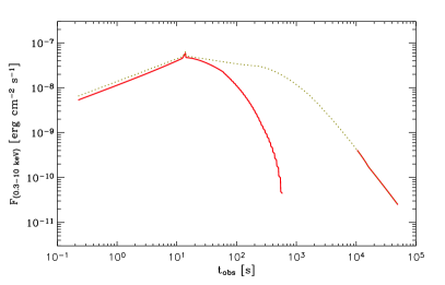
Figure 1: X-ray light curve of a gamma-ray burst located at $z=1$, with fiducial parameters as described at the beginning of Sec. 2; in solid line, result of the model, revealing the flux drop-out at $t_{\rm obs}\sim 100\,$s and the recovery at late times $\sim 10^{4}\,$s. In dotted line, the same model, assuming however that micro-instabilities can grow at all times in front of the forward shock (thus implying $\epsilon_{e}=0.5$, $\epsilon_{B}=0.05$ at all times); this situation also corresponds to what would be seen for magnetizations $\sigma_{\rm u}\,\lesssim\,10^{-6}$, all other parameters remaining unchanged.

Figure 1 presents the resulting light curve in the energy interval $0.3-10\,$keV. The parameters correspond to the previous fiducial values; we have also adopted $\epsilon_{B}=0.05$, $Y_{\rm c}=1$ and $z=1$. At early times, $t_{\rm obs}\,\ll\,10^{4}\,$s, $Y_{\rm inst}>Y_{\rm c}$ hence there is no Fermi power-law, only a thermal electron population extending over half an order of magnitude, implying that the synchrotron emission extends over an order of magnitude. The (observer frame) frequency $\nu_{\rm min}$ associated to $\gamma_{\rm min}$ reads

$$\nu_{\rm min} \simeq \frac{0.2}{1+z}\frac{eB_{\rm b}}{m_{e}c}\gamma_{\rm b}\gamma_{\rm min}^{2}$$ (4)

$$\simeq \frac{1.6\times 10^{18}\,{\rm Hz}}{1+z}\,\,E_{54}^{1/2}A_{*}^{-1/2}T_{1}^{-3/2}B_{*}\epsilon_{e,-1}^{2}\left(\frac{r}{r_{\times}}\right)^{\alpha_{\nu}}\ ,$$

with $\alpha_{\nu}=-1$ for $r<r_{\times}$, $\alpha_{\nu}=-3$ otherwise. Consequently, for $r>r_{\times}$, meaning $t_{\rm obs}>5\,{\rm s}\,(1+z)T_{1}$, the minimum frequency drops rapidly out of the X-ray band. This is accompanied by a drastic reduction in flux as the maximal frequency $\nu_{\rm max}$ ($\sim 9\nu_{\rm min}$ in the absence of Fermi powerlaw) also exits progressively out the X-ray domain. Given the strong dependence of $\nu_{\rm min}$ on $r$, the drop-out occurs shortly after $t_{\times}$: in detail, defining the drop-out time $t_{\rm d-o}$ as that at which $\nu_{\rm min}=0.7\times 10^{17}\,$Hz,

$$t_{\rm d-o}\,\simeq\,110\,{\rm s}\,E_{54}^{1/3}A_{*}^{-1/3}B_{*}^{2/3}\epsilon_{e,-1}^{4/3}(1+z)^{1/3}\ .$$ (5)

This timescale does not depend on the duration of the prompt emission (although it cannot of course be shorter). The shape of the light curve during the drop-out is affected by our assumption of a restricted powerlaw; a more detailed modelling of the electron spectral distribution (e.g. Giannios & Spitkovsky 2009) is required to refine the prediction for the light curve in this region. One should also account for the delay associated with emission away from the ligne of sight or from within the blast, which would lead to a smoothing of the light curve on a timescale $\sim t_{\rm obs}$ at $t_{\rm obs}$.

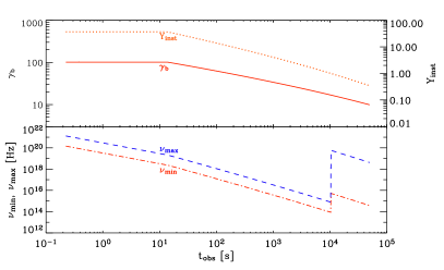
Figure 2: Upper panel: evolution in time of the blast Lorentz factor (left $y-$axis) and of the instability parameter $Y_{\rm inst}$ (right $y-$axis); the onset of Fermi acceleration occurs when $Y_{\rm inst}<1$ in the model shown in Fig. 1, corresponding to $t_{\rm obs}\simeq 10^{4}\,$s. Lower panel: evolution with time of the minimal and maximal observer frame electron synchrotron frequencies; at times $<10^{4}\,$s, Fermi acceleration does not take place, a powerlaw cannot develop hence $\nu_{\rm max}$ is $\sim 1$ order of magnitude larger than the frequency $\nu_{\rm min}$. Note that $\nu_{\rm min}$ exits the X-ray band around $t_{\rm obs}\sim 100\,$s. At late times, Fermi powerlaws develop and the range $\nu_{\rm min}-\nu_{\rm max}$ broadens significantly, leading to the recovery of the standard light curve.

The above simplified model predicts no flux in the X-ray band between the completion of the drop-out, roughly a factor of a few beyond $t_{\rm d-o}$ and the recovery, i.e. the time at which $Y_{\rm inst}=Y_{\rm c}$. This latter timescale $t_{\rm rec}$ can be written

$$t_{\rm rec}\,\simeq\,0.9\times 10^{4}\,{\rm s}\,E_{54}A_{*}^{-3}B_{*}^{4}Y_{\rm c}^{-2}\xi_{\rm b,-1}^{-2}(1+z)\ .$$ (6)

At $t_{\rm rec}$, Fermi cycles develop on a very short timescale compared to the dynamical timescale, hence emission can take place up the maximal frequency $\nu_{\rm max}$ corresponding to $\gamma_{\rm max}$, with

$$\nu_{\rm max}\,\simeq\,7.6\times 10^{18}\,{\rm Hz}\,E_{54}^{-1}A_{*}^{11/2}B_{*}^{-8}Y_{\rm c}^{3}\epsilon_{B,-1.3}^{5/2}\xi_{\rm b,-1}^{3}\left(\frac{t}{t_{\rm rec}}\right)^{-3/2}\ .$$ (7)

The strong dependence of this maximal frequency on the parameters suggests that a variety of effects could take place; in particular, one might observe a weak recovery in the X-ray band or even no recovery at all. Caution has to be exerted however, since when $t_{\rm obs}\gtrsim 10^{4}\,$s the Lorentz factor of the blast has dropped to moderate values $\sim 20$, hence additional effects may come into play. In particular, one cannot rule out the emergence of new instabilities at scales larger than $\delta_{\rm i}$ that would push $\gamma_{\rm max}$ hence $\nu_{\rm max}$ to much larger values. At even later times, jet sideways expansion affects the dynamical evolution; as the above one dimensional model ignores such effects, we stop the calculation at $t=10^{5}\,$s.

Figure 2 summarizes the evolution with $t_{\rm obs}$ of the main parameters and allows to understand better the behaviour of the X-ray light curve shown in Fig. 1. Note that one does not expect a drop-out in the optical, since $\nu_{\rm max}\gtrsim 10^{15}\,$Hz for the present fiducial values and $\nu_{\rm min}$ crosses the optical shortly before $t_{\rm rec}$. Such a drop-out could only be seen if $t_{\rm rec}$ were made much larger than $10^{4}\,$s, e.g. by increasing the magnetization, see Eqs. (4),(5),(6).

4 Discussion

Using “ab initio” principles of relativistic Fermi acceleration now tested in extensive PIC shock simulations, we have calculated the X-ray afterglow light curve of a GRB propagating in a magnetized stellar wind of magnetization $\sigma_{\rm u}\sim 10^{-4}$, assuming otherwise standard GRB parameters. We have shown that the inhibition of relativistic Fermi acceleration in magnetized shocks at high Lorentz factor leaves a distinct signature in the light curve, in the form of a fast drop-out shortly after the end of the prompt emission, around $t_{\rm obs}\sim 100\,$s, with a recovery at late times $\sim 10^{4}\,$s. The latter depends more strongly on the model parameters, in particular magnetization so that one may envisage a variety of situations beyond that described: e.g., no drop-out if $\sigma_{\rm u}\lesssim 10^{-6}$ – ceteris paribus – or a drop-out with no recovery if $\sigma_{\rm u}\gtrsim 10^{-3}$. Although we have calculated the light curve for a stellar wind profile, similar effects might be observed for a constant density circumburst medium, provided the magnetization is large enough. In particular, one would observe a drop-out at $t_{\rm d-o}\simeq 180\,{\rm sec}\,(1.+z)^{1/3}B_{-3}^{2/3}E_{54}^{1/3}n_{0}^{-1/3}\epsilon_{e,-1}^{4/3}$ for a magnetic field $B=10^{-3}B_{-3}\,$G and density $n=n_{0}\,$cm^-3, followed by recovery at $t_{\rm rec}\simeq 10^{4}\,{\rm sec}\,(1.+z)B_{-3}^{8/3}E_{54}^{1/3}n_{0}^{-5/3}Y_{\rm c}^{-4/3}\xi_{{\rm b},-1}^{-4/3}$. Therefore the present results extend beyond the stellar wind case and may be applicable to both long and short GRBs.

Interestingly, recent Swift observations have revealed a rather complex early X-ray afterglow light curve in a subset of GRBs, with a fast decay at $t_{\rm obs}\sim 100\,$s followed by a form of plateau that joins a more standard light curve at later times $\gtrsim 10^{4}\,$s (Nousek et al. 2006, O’Brien et al. 2006). High latitude emission is considered as a possible explanation for the steep decay phase, although modelling the plateau phase with the afterglow brings in additional constraints on the overall GRB model (e.g. Panaitescu 2007). The present scenario could account for two of these observed features – the initial fast decay and the late time recovery – but it does not explain the emergence of the plateau. The following briefly addresses these issues in turn.

Regarding the fast decay phase, the present scenario predicts an exponential decay and a clear spectral transition from hard to soft as the peak of the emission exits the X-ray band. One does not therefore expect a perfectly smooth transition from the prompt emission to the fast decay phase. As discussed in Sec. 3, additional theoretical developments are required to provide a detailed light curve around $100\,$s. Nevertheless, it is of interest to note that Sakamoto et al. (2007) have reported evidence for an exponential decay component on top of a powerlaw decaying component in the early X-ray light curve. Furthermore Zhang et al. (2007) have observed a pronounced hard-to-soft spectral transition during the fast decay in two thirds of GRBs that show a fast decay (see also Yonetoku et al. 2008). Their phenomenological model involves an exponentially cut-off energy spectrum, the peak energy $E_{\rm c}$ of which moves out of the X-ray band during the fast decay according to $E_{\rm c}\propto t_{\rm obs}^{-\alpha_{\rm c}}$ with $\alpha_{\rm c}\simeq 1-1.5$. This fits quite well the present picture, considering in particular that $\nu_{\rm min}\propto t_{\rm obs}^{-1.5}$ [Eq. (4)]. We also note that some short GRBs show an exponentially decaying light curve around 100s, well beyond the prompt emission, accompanied by spectral evolution, such as GRB050724 (Campana et al. 2006), while some show fast decay without apparent late time recovery (e.g. GRB051210, GRB060801, see Nakar 2007).

Regarding the shallow decay phase, a contribution from the reverse shock has been envisaged in Uhm & Beloborodov (2007) and Genet et al. (2007), although some tuning appear required to ensure a smooth transition to the recovery phase. After the present work was submitted, a paper by Petropoulou et al. (2011) appeared, arguing that the shallow decay phase can be accounted for by the low energy tail of the synchrotron self Compton component. Alternatively, one could try to explain the shallow decay phase with an inefficient contribution of the forward shock, the efficiency increasing with time and reaching its maximum at recovery of the standard light curve. This could be accomplished if a small fraction $\chi\epsilon_{e}$ with $\chi\ll 1$ is stored in an accelerated electron powerlaw at that time – beyond the thermal component that amounts to $\epsilon_{e}(1-\chi)\sim\epsilon_{e}$ – with $\chi$ rising up to $\sim 1$ at recovery. Granot et al. (2006) and Ioka et al. (2006) have proposed a similar scenario, with varying microphysical parameters during the shallow decay phase. Our model assumes a sharp transition at $Y_{\rm inst}=1$ between no acceleration (i.e. $\chi=0$) and fully efficient acceleration ($\chi=1$), but what actually happens at $Y_{\rm inst}\sim{\cal O}(1)$ when a few efolds of growth of the turbulence can occur is not known, since we have at our disposal the results of only two simulations at $\sigma_{\rm u}=10^{-4}$ and $10^{-5}$. Moreover, one should recall that current PIC simulations probe tiny timescales in regards of the GRB timescales and that these simulations do not yet converge to a stationary shock state (Keshet et al. 2009). One thus cannot exclude that inefficient acceleration occurs at $Y_{\rm inst}\sim{\cal O}(1)$ but goes undetected in current simulations; dedicated PIC simulations on long timescales appear required to probe this transition region. Alternatively, if the jet is structured in energy and Lorentz factor per solid angle, an observer may receive emission from regions of different Lorentz factors than that on the line of sight (e.g. Panaitescu 2007); if the Lorentz factors in those off-axis regions are such that $Y_{\rm inst}<Y_{\rm c}$, one might detect low flux emission, corresponding to $\chi<1$ and possibly a shallow decay phase. Yet another possibility is that of a clumpy circumburst medium, with clumps of various sizes, provided $r_{\rm c}\,\ll\,r/\gamma_{\rm b}$ . As the causal region of lateral extent $r/\gamma_{\rm b}$ contains many clumps, one does not expect a bumpy signature in the light curve. However, one would collect only a fraction $\chi<1$ of the expected X-ray flux due to acceleration in the fraction $f_{\rm c}<1$ of the clumps that carry a magnetization such that $Y_{\rm inst}<Y_{\rm c}$ at a given time. As the overall density and Lorentz factor decrease, $f_{\rm c}$ increases and so does $\chi$ until recovery, which corresponds to $Y_{\rm inst}\lesssim Y_{\rm c}$ in the smallest scale clumps that carry most of the mass. In each of the above scenarios, one would expect a smooth transition in the light curve with no spectral evolution between the shallow decay phase and the late time normal decay phase, as reported by Nousek et al. (2006) and O’Brien et al. (2006).

More work is certainly warranted to discuss these aspects in more detail and to compare the properties of the light curve to observational data in the relevant wavelength domains. One may in particular expect the inverse Compton GeV emission to provide further constraints on the present scenario.

Acknowledgments: we acknowledge support from the CNRS PEPS/PTI Program and from the GDR PCHE.

References

- [] Beloborodov, A., 2005, ApJ, 627, 346
- [] Beloborodov, A., Uhm, L., 2006, ApJ, 651, L1
- [] Begelman, M. C., Kirk, J. G., 1990, ApJ, 353, 66
- [] Campana, S., Tagliaferri, G., Lazzati, D. et al., 2006, AA, 454, 113
- [] Genet, F., Daigne, F., Mochkovitch, R., 2007, MNRAS, 381, 732
- [] Giannios, D., Spitkovsky, A., 2009, MNRAS, 400, 330
- [] Granot, J., Königl, A., Piran, T., 2006, MNRAS, 370, 1946
- [] Gruzinov, A., Waxman, E., 1999, ApJ, 511, 852
- [] Ignace, R., Cassinelli, J. P., Bjorkman, J. E., 1998, ApJ, 505, 910
- [] Ioka, K., Toma, K., Yamazaki, R., Nakamura, T., 2006, AA, 458, 7
- [] Keshet, U., Katz, B., Spitkovsky, A., Waxman, E., 2009, ApJ, 693, L127
- [] Lemoine, M., Pelletier, G., Revenu, B., 2006, ApJ, 645, L129
- [] Lemoine, M., Pelletier, G., 2010, MNRAS, 402, 321
- [] Lemoine, M., Pelletier, G., 2011, arXiv:1102.1308
- [] Levinson, A., 2010, ApJ, 705, L213
- [] Li, Z., Waxman, E., 2006, ApJ, 651, L328
- [] Li, Z., 2010, arXiv:1004.0791
- [] Medvedev, M. V., Loeb, A., 1999, ApJ, 526, 697
- [] Mészáros, P., Rees, M., 1997, ApJ, 476, 232
- [] Nakar, E., 2007, Phys. Rep., 442, 166
- [] Niemiec, J., Ostrowski, M., Pohl, M., 2006, ApJ, 650, 1020
- [] Nousek, J. A., Kouveliotou, C., Grupe, D. et al., 2006, ApJ, 642, 389
- [] O’Brien, P. T., Willingale, R., Osborne, J. et al., 2006, ApJ, 647, 1213
- [] Owocki, S., 2011, Bull. Soc. Roy. Sc. Liège, vol. 80, p. 16
- [] Panaitescu, A., 2007, MNRAS, 379, 331
- [] Pelletier, G., Lemoine, M., Marcowith, A., 2009, MNRAS, 393, 587
- [] Petropoulou, M., Mastichiadis, A., Piran, T., 2011, AA, 531, 76
- [] Piran, T., 2005, Rev. Mod. Phys., 76, 1143
- [] Ramirez-Ruiz, E., Nishikawa, K.-I., Hededal, C. B., 2007, ApJ 671, 1877
- [] Sakamoto, T., Hill, J. E., Yamazaki, R. et al., 2007, ApJ 669, 1115
- [] Sari, R., Esin, A. A., 2001, ApJ, 548, 787
- [] Sari, R., Piran, T., 1995, ApJ, 455, L143
- [] Sironi, L., Goodman, 2007, ApJ, 671, 1858
- [] Sironi, L., Spitkovski, A., 2011, ApJ, 726, 75
- [] Spitkovsky, A., 2008, ApJ 673, L39
- [] Uhm, L., Beloborodov, A., 2007, ApJ, 665, L93
- [] Yonetoku, D. Tanabe, S., Murakami, T. et al., 2008, PASJ, 60, 352
- [] Zhang, B.-B., Liang, E.-W., Zhang, B., 2007, ApJ, 666, 1002