Changes of Interatomic Force Constants Caused by Quantum Confinement Effects: Study on the Calculations for the First-order Raman Spectrum of Si Nanocrystals in Comparison with Experiments.

Abstract

The redshifts and asymmetric broadening observed in nanocrystal Raman Spectra are attributed to the quantum confinement effects by some authors. But others show that they may come from the local heating caused by the incident laser as well. In this study we demonstrate that in the Si nanocrystal case the latter at most has obvious effects on the broadening but has negligible effects on the 1LO peak shift, while the former contributes most of the 1LO peak shift. We also demonstrate that after assigning appropriate interatomic force constants in the calculation of Raman Spectrum by bond polarizability approximation model within the regime of free boundary condition, we may acquire the matching 1LO peak shift with experiments.

I


Introduction

Attributed to its compatibility to the state-of-the-art semiconductor manufacturing process and the abundance of silicon in nature, silicon nanocrystals, or in a more favorable name, quantum dots, raise world-wide interests for decades in studying their quantum confinement effects on electronic and optical propertiesPRB 47 1397 1993 ${}^{\text{-}}$laser photonic review because of the promising applications to devices such as the light emitting diodesJ Lum 80 263 1999 and single electron transistorsSuperlattices and Microstructures 28 177 2000 . In addition, the vibrational properties of the Si nanocrystals also attract great attentionJAP 78 6705 1995 ${}^{\text{-}}$PRB 80 193410 2009 . For one thing, Raman spectroscopy is a noninvasive technique to investigating defects or qualities of devices. For example, the first order Raman shifts may be used to examine the crystalline quality of the silicon nanostructuresnanotech 18 175705 2007 ${}^{\text{,}}$JAP 90 4175 2001 . On the other hand, studies on electron-phonon coupling and thermodynamic properties of silicon nanocrystals require full understandings for the behaviors of phonon confinements. In comparisons with the first order Raman shifts, the second order Raman shifts may be enhanced by electrochemically etched silicon substrates that are immersed in different duration of timeChem Phys Letter 382 502 2003 . Likewise, Si nanocrystals made by annealing hydrogenated amorphous silicon($\alpha$-Si:H) with continuous-wave laser are also used to study the first and the second Raman spectraPRB 64 073304 .

In study of the first-order Raman Spectrum of Silicon nanocrystals, there are at least two prominent phenomena to which we should pay attention. First, the asymmetric broadening towards low frequency around 1LO transition (520 cm${}^{\text{-1}}$for bulk) is observed in the spectrum, indicating a phonon confinement effect. Secondly, the (bulk) 520 cm${}^{\text{-1}}$ peak shift to lower frequency with reducing nanocrystal sizes. There have been extensive theoretical and experimental studies of the first-order nanocrystal Raman scattering. H.Richter et.al.Richter's , describes a phenomenological exponential function that restricts the nanocrystal phonon wavefunctions in the sphere. Several different weighting functions are also usedSSC Campbell and Fauchet ${}^{\text{-}}$PRB 73 033307 2006 . However, even though it is claimed that experimental data could be well explained by the above method, it is still obscure for the exponential and weighting functions to have definitive physical meanings so that they may not provide information of interatomic physical quantities. Therefore, it could be more preferable that we start from solving the characteristic vibrations of the nanocrystal, which contribute to the change of polarizability resulting in the Raman effects. Thus, the bond polarizability approximationBPA Bell (BPA) is introduced to calculate the first-order Raman Spectrum of SiCheng and Ren as well as fullereneBPA fullerene . This model suggests that the total polarizability tensor is the sum over each axially symmetric polarizability tensor connecting each pair of atoms $ij$, for which may be expressed as a function of two bond-length dependent parameters, one referring to mean polarizability while the other anisotropic polarizability. The total polarizability tensor is then approximated up to the first order with respect to the equilibrium position of the atoms. However, the asymmetric broadening effect does not meet agreement with the experimental results in the calculation.

Failure to success may be imputed to several reasons. First, it is difficult to obtain appropriate interatomic force constants (IFCs) among atoms by only considering the first-neighbor interactions, resulting in unsuitable phonon eigenfrequencies and eigenvectors. Improvements may be made by considering the IFCs up to the second neighbors. Secondly, there seems no reason to only consider the first-neighbor atoms in the parameters of bond polarizability. Thirdly, some studies show that the peak shift and asymmetric broadening may be due to local heating from the tiny focusing laser spot rather than size effectsPRB 80 193410 2009 ${}^{\text{,}}$PRB 66 161311R 2002 local heating . However, since both of the parameters of bond polarizability and the IFCs cannot be known in priori, it is difficult to obtain proper values of them without comparing the peak shift of experiments. Therefore, close agreement of asymmetric broadening in concomitant of the peak shift towards low frequencies between calculations and experiments remains challenging.

In this study, we first obtain IFCs by fitting the bulk silicon dispersion relations calculated by the rigid-ion modelRIM up to the second nearest neighbors with the experimental data from the neutron scattering at the three special points, $\Gamma$, $X$, and $L$, in the First Brillouin zone. The IFCs are then compared with the results from ab initio calculations in order to show the significance of the parameters. Afterwards, these fitting parameters are used to calculate the vibrational properties in nanocrystals by little modification with the self energy of the surface atoms. Nanocrystals with two different diameters are made and measured by Raman spectrometer with He-Ne and Argon-ion lasers. Peak shift and broadening effect regarding to the nanocrystal sizes or laser power variations are discussed. The first order Raman spectra are calculated by bond polarizability approximation (BPA)BPA Bell . It is found that we may acquire close peak shift by assigning proper IFCs in the calculation and obtain more satisfactory asymmetric broadening effects by considering the parameters of polarizability up to the second-nearest neighbor atoms. Fair resemblance to the calculated first-order Raman spectra with the experimental ones is seen.

II Theory and Sample Preparations

II.1 The Rigid-ion Model and Interatomic Force Constants in Bulk

For a homopolar Silicon bulk crystal, the potential energy $U$ is expanded up to the second order harmonic approximation with respect to the equilibrium position of an atom. This term, $\frac{\partial^{2}U}{\partial u_{i}\partial u_{j}}|_{\overset{\rightharpoonup}{x_{0}}}$, is then described as the dynamic matrix $D_{jj^{\prime}}^{\sigma\sigma^{{}^{\prime}}}$in the eigenvalue problem,

$$\underset{\sigma^{{}^{\prime}}j^{\prime}}{{\displaystyle\sum}}D_{jj^{\prime}}^{\sigma\sigma^{{}^{\prime}}}(\overset{\rightharpoonup}{q})u_{j^{\prime}}^{\sigma^{{}^{\prime}}}=M_{\sigma}\omega^{2}(\overset{\rightharpoonup}{q})u_{j}^{\sigma}$$ (1)

, where $\sigma$ denotes different kinds of atoms in a unit cell and $j^{{}^{\prime}}$ denotes x,y,z in Cartesian coordinates, $M_{\sigma}$ being the mass of the atom for each kind. Furthermore, for periodicity in bulk,

$$D_{jj^{\prime}}^{\sigma\sigma^{{}^{\prime}}}(\overset{\rightharpoonup}{q})=\underset{\overset{\rightharpoonup}{R}}{{\displaystyle\sum}}D_{jj^{\prime}}^{\sigma\sigma^{{}^{\prime}}}(\overset{\rightharpoonup}{R}+\overset{\rightharpoonup}{S}_{\sigma}-\overset{\rightharpoonup}{S}_{\sigma^{\prime}})e^{i\overset{\rightharpoonup}{q}\cdot(\overset{\rightharpoonup}{R}+\overset{\rightharpoonup}{S}_{\sigma}-\overset{\rightharpoonup}{S}_{\sigma^{\prime}})}$$ (2)

, where $\overset{\rightharpoonup}{R}$ denotes the position vectors of the first-neighbour or second-neighbour atom and $\overset{\rightharpoonup}{S}_{\sigma}$denotes the vectors in which the atom in the primitive unit cell with species $\sigma$ resides. In the rigid-ion modelRIM , the term $D_{jj^{\prime}}^{\sigma\sigma^{{}^{\prime}}}(\overset{\rightharpoonup}{R}+\overset{\rightharpoonup}{S}_{\sigma}-\overset{\rightharpoonup}{S}_{\sigma^{\prime}})$ is described by several 3 by 3 force-constant matrices. Specifically, the 3 by 3 matrix for the first-nearest neighbour atom at the position $\frac{a}{4}(1,1,1)$ is defined by

$$D^{1,2}(1)=\left(\begin{array}[c]{ccc}A&B&B\\ B&A&B\\ B&B&A\end{array}\right)$$ (3)

, and for the second-nearest neighbour atom at the position $\frac{a}{4}(2,2,0)$ we define

$$D^{\sigma\sigma}(1)=\left(\begin{array}[c]{ccc}C&D&E\\ D&C&E\\ -E&-E&F\end{array}\right)$$ (4)

. For all the other atoms at the position $\overset{\rightharpoonup}{R}$, the relative force-constant matrices may be derived by similarity transformation $D^{\sigma\sigma^{{}^{\prime}}}(\overset{\rightharpoonup}{R})=T_{i}D^{\sigma\sigma^{{}^{\prime}}}(1)T_{i}^{-1}$ with orthogonal matrix $T_{i}$ of determinant 1book methods in computational physics . Here only up to second-order nearest neighbours are taken into consideration. We derive the eigenvalues at the $\Gamma,X,L$ points in the Brillouin zonePRB 74 054302 2006 .

For $\overset{\rightharpoonup}{q}=\Gamma$, the eigenvalues are  $0$ and $-8A$, both being triplet degenerate. For $\overset{\rightharpoonup}{q}=X$ at $(1,0,0)$, we have

$$-4A-16C\text{ ; one LO and one LA}$$ (5a)

$$-4A-4B-8C-8F\text{ ; two TO}$$ (5b)

$$-4A+4B-8C-8F\text{ ; two TA}$$ (5c)

They are all double degenerate. At last, for the $L$ point $(\frac{1}{2},\frac{1}{2},\frac{1}{2})$, we have

$$-6A-2B-8C+4D-4F\text{ ; two TO}$$ (6a)

$$-6A+4B-8C-8D-4F\text{ ; one LO}$$ (6b)

$$-2A-4B-8C-8D-4F\text{ ; one LA}$$ (6c)

$$-2A+2B-8C+4D-4F\text{ ; two TA}$$ (6d)

$A,B,C,F$ are solved unambiguously at $\Gamma$ and $X$. Unfortunately one may immediately notice that there is no value for $D$ that may simultaneously satisfy Eq 6. Furthermore, there is no information for $E$ at the three special points. However, one may obtain values of $D$ and $E$ by calculating the interatomic force constants with ab initio calculations. We use linear responsePhys Rev B 55 10337 1997 ${}^{\text{,}}$Phys Rev B 55 10355 1997 implantation of DFT with a local density approximation (LDA) to exchange correlation effect and Troullier-Martins pseudopotential in Abinit codeComputer Phys Commun 180 2582 2009 ${}^{\text{,}}$Zeit Kristallogr 220 558 2005 . The cutoff energy is set to 30 hatrees for the plane-wave basis. Two sets of the parameters obtained either by directly solving the multiple equations above, from plugging in neutron scattering experiment datadata1 ${}^{\text{,}}$data2 , or by the ab initio calculations are summarized and compared in Table I. The phonon density of states with even-grid k pointseven grided k points in the first Brillouin zone and phonon dispersion relations are shown in Fig 1.

One researcher said that the parameter $E$ in the IFCs is zero because “for Group IV, we must have $E_{1}$ $=$ $E_{2}$ $=0$ to preserve symmetry.” While in compounds such as AlAs or GaAs, as well as for superlattice, $E_{1}$ and $E_{2}$ are also assigned to be zero in their studies. The reason why this is incorrect and how they made this mistake will be discussed in Appendix.

II.2 Calculations on Nanocrystals Eigenvalue Problems

An atom in a nanocrystal is called the bulk atom when there are 4 first-nearest neighbours and 12 second-nearest neighbours surrounding it, while an atom that does not fulfill this criterion is called the surface atom. Accurate and satisfactory interatomic force constants of every atom in a nanocrystal may be obtained by fully considering the minimum value of the forces of constraint with arbitrary displacements of atoms in the nanocrystalmethod of relaxation , known as the “relaxation method.” Nevertheless, with an optimistic simplicity one may place the assumption that the interatomic force constants of Silicon atoms in a nanocrystal may have close values to those in bulk, except a slight modification at the surface atoms of the nanocrystal. The assumption is reasonable because in bulk we only consider that a Si atom is influenced at most by its first and second nearest neighbours, leaving outer neighbours invisible. Therefore as long as the size of the nanocrystal under consideration is not too small, the force constants from bulk may still apply to the nanocrystal.

At the absence of periodicity, the dynamic matrix of a nanocrystal consisting of $N$ atoms is expanded to a $3N\times 3N$ square matrix. The dynamic matrix is constructed in such a way that each $3$ by $3$ block representing the mutual force constants between atom $i$ and atom $j$ is placed in positions designating the rows $(i-1,i,i+1)$ and columns $(j-1,j,j+1)$ in the dynamic matrix. The $3\times 3$ diagonal block placed at the rows $(i-1,i,i+1)$ and columns $(i-1,i,i+1)$ in the dynamic matrix is understood as the self energy of the atom $i$, which is discussed below.

For bulk, the self-energy of an atom is determined by noticing that the net force exerted on an atom at the position $(\overset{\rightharpoonup}{R}+\overset{\rightharpoonup}{S}_{\sigma})$ ,

$$\sum_{\overset{\rightharpoonup}{R^{{}^{\prime}}},\sigma^{\prime}}D^{\sigma\sigma^{{}^{\prime}}}(\overset{\rightharpoonup}{R}+\overset{\rightharpoonup}{S}_{\sigma}-\overset{\rightharpoonup}{R^{{}^{\prime}}}-\overset{\rightharpoonup}{S}_{\sigma^{\prime}})\cdot u^{\sigma^{{}^{\prime}}}(\overset{\rightharpoonup}{R^{{}^{\prime}}})$$ (7)

, vanishes when the atom is at the equilibrium position $\overset{\rightharpoonup}{d}$. Thus,

$$\sum_{\overset{\rightharpoonup}{R},\sigma^{\prime}}D^{\sigma\sigma^{{}^{\prime}}}(\overset{\rightharpoonup}{R}+\overset{\rightharpoonup}{S}_{\sigma}-\overset{\rightharpoonup}{S}_{\sigma^{\prime}})=0$$ (8)

. This gives

$$D^{\sigma\sigma}(\overset{\rightharpoonup}{0})=-\sum_{\overset{\rightharpoonup}{R}\neq\overset{\rightharpoonup}{0},\sigma^{\prime}}D^{\sigma\sigma^{{}^{\prime}}}(\overset{\rightharpoonup}{R}+\overset{\rightharpoonup}{S}_{\sigma}-\overset{\rightharpoonup}{S}_{\sigma^{\prime}})$$ (9)

. In other words, the self energy of an atom is the negative sign of the sum of the 3 by 3 force-constant matrices of the atoms surrounding it. In bulk, the self energy is thus

$$D^{\sigma\sigma}(\overset{\rightharpoonup}{0})=-4(A_{\sigma}+2C_{\sigma}+F_{\sigma})I$$ (10)

Eq 9 also holds for nanocrystals by modification of the equilibrium position for atoms after relaxation. Therefore, for the self energy of surface atoms that have no 16 ambient atoms in the nanocrystal we simply sum up the 3 by 3 force-constant matrices of the ambient atoms. It may be recognized as the free boundary condition after we make the self energy of surface atoms in this way. The central force assumption up to the second-neighbor atoms, $E=0$RIM , is assumed for surface atoms in order to preserve symmetry in the dynamic matrix. Afterwards, the standard procedure of solving the eigenfrequencies and eigenvectors of the dynamic matrix is applied. Knowledge of group theory regarding to $T_{d}$ group is implemented to the dynamic matrix. This dramatically ameliorates the requirements of computer memory and reduces time needed to solve the eigenvalue problem of the dynamic matrix. Very few number of negative eigenvalues are found because we did not relax the nanocrystals. For example, 2 out of 3317 modes in the $T_{2}$ representation of the 7nm case are found to be negative with the imaginary parts $0.494$ THz and $0.008$ THz. We neglect these kinds of modesJ Phys Condens Matter 20 145213 2008 .

II.3 Bond Polarizability Approximation and Intensity of the Raman Spectrum

The issue that lies at the heart of the vibrational Raman effects is the change of polarizability of the nanocrystal on which we measure. The total polarizability tensor $\alpha_{\rho\sigma}^{tot}$, where $\rho$ and $\sigma$ refer to the Cartesian coordinate index, is readily understood by summing over every polarizability tensor $\alpha_{\rho\sigma}$($\overset{\rightharpoonup}{\rho_{ij}}$) connecting atom $i$ and atom $j$:

$$\alpha_{\rho\sigma}^{tot}=\underset{i<j}{\sum}\alpha_{\rho\sigma}(\overset{\rightharpoonup}{\rho_{ij}})$$ (11)

Bond polarizability approximation (BPA) modelBPA Bell suggests that one may write the polarizability tensor for each bond $\alpha_{\rho\sigma}$($\overset{\rightharpoonup}{\rho_{ij}}$) as

$$\alpha_{\rho\sigma}(\overset{\rightharpoonup}{\rho_{ij}})=\alpha(\overset{\rightharpoonup}{\rho_{ij}})I+\gamma(\overset{\rightharpoonup}{\rho_{ij}})(\overset{\wedge}{\rho_{ij}}\overset{\wedge}{\rho_{ij}}-\frac{1}{3}I)$$ (12)

, where $\alpha(\overset{\rightharpoonup}{\rho_{ij}})$ and $\gamma(\overset{\rightharpoonup}{\rho_{ij}})$ are isotropic and anisotropic polarizabilities (called the polarizability parameters) as a function of position vector associating with atom $i$ and atom $j$, $\overset{\rightharpoonup}{\rho_{ij}}$, respectively. $I$ is $3\times 3$ unit matrix and $\overset{\wedge}{\rho_{ij}}$ refers to the unit vector of $\overset{\rightharpoonup}{\rho_{ij}}$. As the nanocrystal is excited by incident light the characteristic motion of each atom vibrates with a certain eigenfrequency $w_{l}$ away from its own original equilibrium position, therefore the position vector between atom $i$ and atom $j$ changes to $\overset{\rightharpoonup}{\rho_{ij}}=\overset{\rightharpoonup}{r_{ij}}+\overset{\rightharpoonup}{x_{ij}}$with a slight relative movement $\overset{\rightharpoonup}{x_{ij}}$ ( more specifically, the relative eigenvectors for atom $i$ and atom $j$ corresponding to the eigenfrequency $w_{l}$) displacing away from the relative equilibrium position $\overset{\rightharpoonup}{r_{ij}}$. For harmonic vibrations we may expand Eq 12 with respect to $\overset{\rightharpoonup}{x_{ij}}$ up to the first order under the assumption that $\overset{\rightharpoonup}{x_{ij}}\ll\overset{\rightharpoonup}{r_{ij}}$. First notice that, up to the first order,

$$\overset{\wedge}{\rho_{ij}}\overset{\wedge}{\rho_{ij}} =\frac{(\overset{\rightharpoonup}{r_{ij}}+\overset{\rightharpoonup}{x_{ij}})(\overset{\rightharpoonup}{r_{ij}}+\overset{\rightharpoonup}{x_{ij}})}{\left|\overset{\rightharpoonup}{r_{ij}}+\overset{\rightharpoonup}{x_{ij}}\right|^{2}}$$

$$\approx r_{ij}^{-2}\left[1-\frac{2(\overset{\wedge}{r_{ij}}\cdot\overset{\rightharpoonup}{x_{ij}})}{r_{ij}}\right](\overset{\rightharpoonup}{r_{ij}}+\overset{\rightharpoonup}{x_{ij}})(\overset{\rightharpoonup}{r_{ij}}+\overset{\rightharpoonup}{x_{ij}})$$ (13)

. Secondly we have the expansion for $\alpha(\overset{\rightharpoonup}{\rho_{ij}})$ up to the first order as

$$\alpha(\overset{\rightharpoonup}{r_{ij}}+\overset{\rightharpoonup}{x_{ij}})=\alpha(\overset{\rightharpoonup}{r_{ij}})+\alpha^{{}^{\prime}}(\overset{\rightharpoonup}{r_{ij}})(\overset{\rightharpoonup}{x_{ij}}\cdot\overset{\wedge}{r_{ij}})\text{, where }\alpha^{{}^{\prime}}(\overset{\rightharpoonup}{r_{ij}})=\frac{\partial\alpha(\overset{\rightharpoonup}{\rho_{ij}})}{\partial\overset{\rightharpoonup}{x_{ij}}}|_{\overset{\rightharpoonup}{\rho_{ij}}=\overset{\rightharpoonup}{r_{ij}}}$$ (14)

. Similar formula applies to $\gamma(\overset{\rightharpoonup}{\rho_{ij}})$. This leads to the first-order expansion of Eq 12 as the following:

$$\alpha_{\rho\sigma}(\overset{\rightharpoonup}{r_{ij}}+\overset{\rightharpoonup}{x_{ij}}) \approx\alpha(\overset{\rightharpoonup}{r_{ij}})+\alpha^{{}^{\prime}}(\overset{\rightharpoonup}{r_{ij}})(\overset{\rightharpoonup}{x_{ij}}\cdot\overset{\wedge}{r_{ij}})+\left[\gamma(\overset{\rightharpoonup}{r_{ij}})+\gamma^{{}^{\prime}}(\overset{\rightharpoonup}{r_{ij}})(\overset{\rightharpoonup}{x_{ij}}\cdot\overset{\wedge}{r_{ij}})\right]\cdot$$

$$\left[\overset{\wedge}{r_{ij}}\overset{\wedge}{r_{ij}}+\frac{\overset{\wedge}{r_{ij}}}{r_{ij}}\overset{\rightharpoonup}{x_{ij}}+\overset{\rightharpoonup}{x_{ij}}\frac{\overset{\wedge}{r_{ij}}}{r_{ij}}-\frac{2}{r_{ij}}(\overset{\rightharpoonup}{x_{ij}}\cdot\overset{\wedge}{r_{ij}})(\overset{\wedge}{r_{ij}}\overset{\wedge}{r_{ij}}+\frac{\overset{\wedge}{r_{ij}}}{r_{ij}}\overset{\rightharpoonup}{x_{ij}}+\overset{\rightharpoonup}{x_{ij}}\frac{\overset{\wedge}{r_{ij}}}{r_{ij}})-\frac{I}{3}\right]$$

$$\approx\alpha(\overset{\rightharpoonup}{r_{ij}})+\alpha^{{}^{\prime}}(\overset{\rightharpoonup}{r_{ij}})(\overset{\rightharpoonup}{x_{ij}}\cdot\overset{\wedge}{r_{ij}})+\gamma(\overset{\rightharpoonup}{r_{ij}})(\overset{\wedge}{r_{ij}}\overset{\wedge}{r_{ij}}-\frac{I}{3})+\gamma^{{}^{\prime}}(\overset{\rightharpoonup}{r_{ij}})(\overset{\rightharpoonup}{x_{ij}}\cdot\overset{\wedge}{r_{ij}})(\overset{\wedge}{r_{ij}}\overset{\wedge}{r_{ij}}-\frac{I}{3})$$

$$+\gamma(\overset{\rightharpoonup}{r_{ij}})\left[\frac{\overset{\wedge}{r_{ij}}}{r_{ij}}\overset{\rightharpoonup}{x_{ij}}+\overset{\rightharpoonup}{x_{ij}}\frac{\overset{\wedge}{r_{ij}}}{r_{ij}}-\frac{2}{r_{ij}}(\overset{\rightharpoonup}{x_{ij}}\cdot\overset{\wedge}{r_{ij}})\overset{\wedge}{r_{ij}}\overset{\wedge}{r_{ij}}\right]$$

$$\approx\alpha_{\rho\sigma}(\overset{\rightharpoonup}{r_{ij}})+(\overset{\rightharpoonup}{x_{ij}}\cdot\overset{\wedge}{r_{ij}})\left[\alpha^{{}^{\prime}}(\overset{\rightharpoonup}{r_{ij}})I+\gamma^{{}^{\prime}}(\overset{\rightharpoonup}{r_{ij}})(\overset{\wedge}{r_{ij}}\overset{\wedge}{r_{ij}}-\frac{I}{3})\right]$$

$$+\gamma(\overset{\rightharpoonup}{r_{ij}})r_{ij}^{-1}\left[\overset{\wedge}{r_{ij}}\overset{\rightharpoonup}{x_{ij}}+\overset{\rightharpoonup}{x_{ij}}\overset{\wedge}{r_{ij}}-2(\overset{\rightharpoonup}{x_{ij}}\cdot\overset{\wedge}{r_{ij}})\overset{\wedge}{r_{ij}}\overset{\wedge}{r_{ij}}\right]$$

The first term $\alpha_{\rho\sigma}(\overset{\rightharpoonup}{r_{ij}})$ is neglected because it makes no contribution to Raman effects. Thus the total polarizability tensor taken into consideration up to the first-order expansion will be expressed as

$$\alpha_{\rho\sigma}^{tot}{}^{(1)}=\underset{i<j}{\sum}(\overset{\rightharpoonup}{x_{ij}}\cdot\overset{\wedge}{r_{ij}})\left[\alpha^{{}^{\prime}}(\overset{\rightharpoonup}{r_{ij}})I+\gamma^{{}^{\prime}}(\overset{\rightharpoonup}{r_{ij}})(\overset{\wedge}{r_{ij}}\overset{\wedge}{r_{ij}}-\frac{I}{3})\right]+\gamma(\overset{\rightharpoonup}{r_{ij}})r_{ij}^{-1}\left[\overset{\wedge}{r_{ij}}\overset{\rightharpoonup}{x_{ij}}+\overset{\rightharpoonup}{x_{ij}}\overset{\wedge}{r_{ij}}-2(\overset{\rightharpoonup}{x_{ij}}\cdot\overset{\wedge}{r_{ij}})\overset{\wedge}{r_{ij}}\overset{\wedge}{r_{ij}}\right]$$ (15)

. Similarly the expansion of Eq 12 up to the second order may also be derived as

$$\alpha_{\rho\sigma}^{(2)} =\frac{1}{2}(\overset{\rightharpoonup}{x_{ij}}\cdot\overset{\wedge}{r_{ij}})^{2}\left[\alpha^{{}^{\prime\prime}}(\overset{\rightharpoonup}{r_{ij}})I+\gamma^{{}^{\prime\prime}}(\overset{\rightharpoonup}{r_{ij}})(\overset{\wedge}{r_{ij}}\overset{\wedge}{r_{ij}}-\frac{I}{3})\right]$$

$$+\gamma^{{}^{\prime}}(\overset{\rightharpoonup}{r_{ij}})r_{ij}^{-1}(\overset{\rightharpoonup}{x_{ij}}\cdot\overset{\wedge}{r_{ij}})\left[\overset{\wedge}{r_{ij}}\overset{\rightharpoonup}{x_{ij}}+\overset{\rightharpoonup}{x_{ij}}\overset{\wedge}{r_{ij}}-2(\overset{\rightharpoonup}{x_{ij}}\cdot\overset{\wedge}{r_{ij}})\overset{\wedge}{r_{ij}}\overset{\wedge}{r_{ij}}\right]$$

$$+\gamma(\overset{\rightharpoonup}{r_{ij}})r_{ij}^{-2}\left\{\overset{\rightharpoonup}{x_{ij}}\overset{\rightharpoonup}{x_{ij}}+\left[4(\overset{\rightharpoonup}{x_{ij}}\cdot\overset{\wedge}{r_{ij}})^{2}-x_{ij}^{2}\right]\overset{\wedge}{r_{ij}}\overset{\wedge}{r_{ij}}-2(\overset{\rightharpoonup}{x_{ij}}\cdot\overset{\wedge}{r_{ij}})(\overset{\wedge}{r_{ij}}\overset{\rightharpoonup}{x_{ij}}+\overset{\rightharpoonup}{x_{ij}}\overset{\wedge}{r_{ij}})\right\}$$ (16)

, which involves the second derivative of $\alpha$ and $\gamma$ with respect to $\overset{\rightharpoonup}{x_{ij}}$. In this study, Eq 15 will be used to calculate the first-order Raman Spectra for Silicon nanocrystals.

For backscattering detection configuration, at which the propagation direction of the scattered light is parallel but opposite against that of the (linearly polarized) incident light ,

one may obtain the temperature-independent (reduced) intensity of the scattered light regarding to two different polarizations: one for the polarization of the scattered light parallel to that of the incident light ($I_{s,||}$), the other for the polarization of the scattered light perpendicular to that of the incident light ($I_{s,\bot}$). Taken into consideration of averaging over all the possible orientations of nanocrystals for a given radius, we haveBPA Bell ${}^{\text{,}}$book D A LONG :

$$I_{s,||}\varpropto\underset{l}{\sum}g(w_{l})\cdot(4G_{l}^{2}+45A_{l}^{2})$$ (17)

, and

$$I_{s,\bot}\varpropto\underset{l}{\sum}g(w_{l})\cdot 3G_{l}^{2}$$ (18)

, where $g(w_{l})$ is the vibrational spectrum and

$$A_{l}=\frac{1}{3}[\alpha_{11}^{tot}{}^{(1)}+\alpha_{22}^{tot}{}^{(1)}+\alpha_{33}^{tot}{}^{(1)}]$$ (19)

$$G_{l}^{2} =\frac{1}{2}\left\{[\alpha_{11}^{tot}{}^{(1)}-\alpha_{22}^{tot}{}^{(1)}]^{2}+[\alpha_{22}^{tot}{}^{(1)}-\alpha_{33}^{tot}{}^{(1)}]^{2}+[\alpha_{33}^{tot}{}^{(1)}-\alpha_{11}^{tot}{}^{(1)}]^{2}\right\}$$

$$+3\left\{[\alpha_{12}^{tot}{}^{(1)}]^{2}+[\alpha_{23}^{tot}{}^{(1)}]^{2}+[\alpha_{31}^{tot}{}^{(1)}]^{2}\right\}$$ (20)

II.4 Samples Preparations

The silicon nanocrystals are produced under pressures at 0.5 torr, 1 torr, 2 torr, and 4 torr, in which we thermal evaporate the silicon sputtering target put on a glass substrate that is mounted on the Tantalum (Ta) boat. The system first is pumped down to 10${}^{\text{-3}}$ torr, then in tandem, purged with Argon gas three times to remove residual water vapor and oxygen. Details of the fabrication process are described elsewhereSY lin paper 1 ${}^{\text{-}}$SY lin paper 3 . In this situation the silicon atoms form nanocrystals with various sizes, within some standard deviation, in diameters of 7 nm, 13 nm, 31 nm, and 37 nm, respectively. The relationship between the fabrication pressure and the size of Si nanocrystals is discussed by elsewhereTED and TEM graphics . The standard deviations for 7nm and 13nm cases are both roughly 1nm. There is a clear tendency that under higher pressure leads to a larger nanocrystal size. This may be explained by noticing that under higher pressure the higher collision rate is achieved, thus enhancing the migration and nucleation probability of the Si nanocrystals in the inert-gas atmosphere. The crystalline property is investigated by transmission electron diffraction pattern, and nanocrystal sizes are measured by transmission electron microscopyTED and TEM graphics .

III Results and Discussions

III.1
Experimental Details

Raman Spectra of Silicon nanocrystals with two different radii (7 nm and 13 nm in diameter) are measured by 488 nm Argon ion laser on Horiba Jobin-Yvon HR800 UV micro-Raman Spectrometer with the groove density of 1200 grooves/mm. The charge-coupled device detector is cooled down to $-133{{}^{\circ}}C$ by liquid nitrogen. A 100X objective is used to collect the back-scattering signals. Exposure time of 100 seconds and accumulation number of 5 times are required to obtain a clear spectrum in the parallel-polarized configuration for every sample. The laser power is varied from 5mW to 60 mW from the source, resulting in the laser power on the surface of samples ranging from 0.58mW to 5.23mW, which is measured by Thorlabs PM100D optical power and energy meter.

In order to demonstrate the difference in the spectra for polarization dependence, we also study the parallel and perpendicular polarizations by 632.8 nm He-Ne laser. Exposure time and accumulation number are set to 30 seconds and 20 times and the laser power on the sample surface is 1.7 mW in the case. With a resolution of 3.5 cm${}^{\text{-1}}$, intensity of the polarization-dependent scattered light is measured and compared with the calculation from Eq 17 and Eq 18. A standard Silicon chip, treated as the result of bulk Silicon, is also measured and used to calibrate the system to 520 cm${}^{\text{-1}}$.

III.2
Calculations of the Spectra

Before comparing the calculations and experiments, there are some remarks of calculations. First,

we observe that only intensities involving the eigenmodes belonging to $T_{2},$ $E,$ and $A_{1}$ are Raman active among the five irreducible representations $A_{1},$ $A_{2},$ $E,$ $T_{1},$ and $T_{2}$group theory Inui . Second, the overall spectrum for a nanocrystal with a specific diameter is acquired by summing over intensities from every representation and also by taking into consideration the degeneracy of each representation:

$$I_{tot}=I_{A_{1}}\times 1+I_{E}\times 2+I_{T_{2}}\times 3$$ (21)

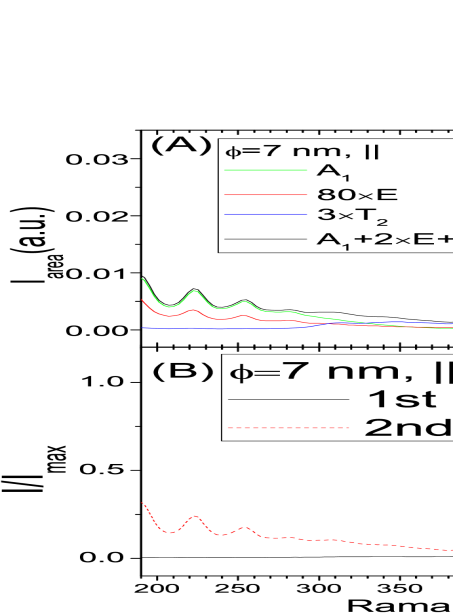
Figure 2: (A) The overall spectrum is the sum of the intensities from the three Raman-active representations after considering the degeneracy of every representation. The curve is for the case with the parameters in the bond polarizability up to the 2nd neighbor. (B) Calculations for parallel polarization of the first-order Raman spectrum when considering the first-order and the second-order neighboring atoms in the bond polarizability parameters.

. Fig 2(A) shows how the three Raman-active representations sum up to a total intensity for the case of parallel polarization for the 7nm case. In spite of this, to be consistent with the second-neighbor consideration for the short-range part in the dynamic matrix when calculating the interatomic force constants, we may also need the second-neighbor parameters of polarizabilities parameters, $\alpha(\overset{\rightharpoonup}{r_{ij}})$ and $\gamma(\overset{\rightharpoonup}{r_{ij}})$. Fig 2(B) shows that the spectrum may be matched well for the asymmetric broadening effect for the parallel polarization when one considers the polarizability parameters, $\alpha(\overset{\rightharpoonup}{r_{ij}})$ and $\gamma(\overset{\rightharpoonup}{r_{ij}})$, up to the second-neighbor atoms. The parameters of the second-neighbor atoms are chosen to satisfy the ordinary differential equations of $\alpha(\overset{\rightharpoonup}{r_{ij}})$ and $\gamma(\overset{\rightharpoonup}{r_{ij}})$BPA Bell . This condition, as well as $\alpha_{c}=\gamma_{c}=0.0001$, is used to calculate the first-order Raman spectra of nanocrystals composed of 8,597 atoms (7 nm in diameter) and 58,125 atoms (13 nm in diameter). Some anomalous peaks in the range 200 cm${}^{\text{-1}}$ to 300 cm${}^{\text{-1}}$ are shown in Fig 2 ( 221 cm${}^{\text{-1}}$, 254 cm${}^{\text{-1}}$, and 281 cm${}^{\text{-1}}$ ) but are not shown in the experiments because they are mainly due to single-size effects thus being smeared out by size deviation in real samples. At last, taking into account the nature of shape of the nanocrystals and the fact that the surface of every nanocrystal is hydrogenated, both resulting in the smaller values of eigenfunctions that stand for the motion of the atoms on the surface, we find that the experiments are well described when we divide the eigenfunctions in the $A_{1}$ and $E$ representations, whose eigenvalues are smaller than 300 cm${}^{-1},$ by 8 for the 7nm case while dividing by 6 for the 13 nm case.

III.3 Comparisons

III.3.1
The Spectra measured by He-Ne Laser

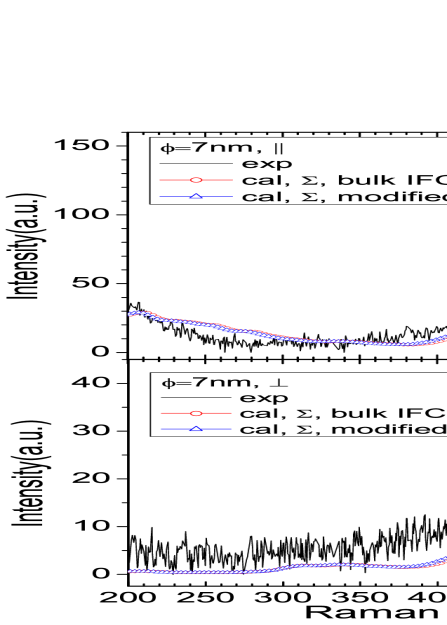
Figure 3: Comparisons of the first-order Raman spectra between calculations(cal) and He-Ne experiments(exp) under parallel ($|$$|$, Fig A) and perpendicular ($\bot$, Fig B) polarizations for nanocrystals of 7 nm in diameter. Single-size peaks from 200 cm${}^{\text{-1}}$ to 300 cm${}^{\text{-1}}$ are smeared out after summing up all the spectra of the size deviations ranging from 6.1 nm to 8.4 nm. (cal, $\sum$). After assigning A=-9.56431, we may get correct peak position. Because Intensity from perpendicular-polarized A₁ modes is zero, the curve is flattened out in the low frequency region in Fig B.

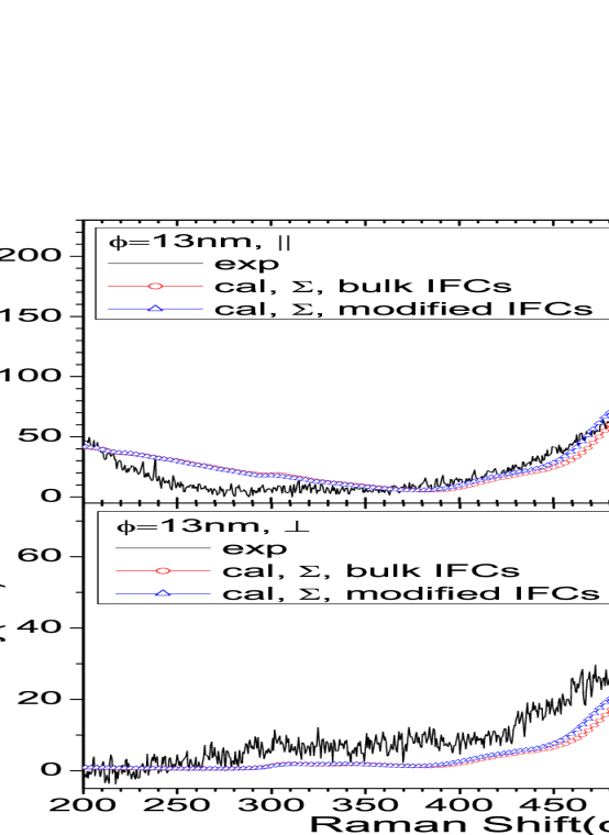
Figure 4: Comparisons of the first-order Raman spectra between calculations(cal) and experiments(exp) under parallel ($|$$|$, Fig A) and perpendicular ($\bot$, Fig B) polarizations for nanocrystals of 13 nm in diameter. After assigning A=-9.58383, we may get correct peak position.

Comparisons with experiments measured by He-Ne laser with satisfying similarities in between are shown in Fig 3 and Fig 4 for the polarization-dependent study. The three anomalous peaks shown in Fig 2 are smeared out after considering the standard deviation ($\sim$1nm) of the 7nm nanocrystal diameters. Notice that when using bulk IFCs, the DOS of the nanocrystal may almost reproduce that of bulk when the nanocrystal size is larger than 6nm, but one immediately recognizes that the mode at 320 cm${}^{\text{-1}}$ shown in the DOS of nanocrystal does not contribute to the first-order Raman spectrum and that the one-phonon effect makes no significant contribution to the lines around 300 cm${}^{\text{-1}}$. Therefore it should be totally due to the two-phonon effect, being recognized as 2TAPRB 64 073304 ${}^{\text{,}}$two phonons in si bulk . For both cases, the DOS curves have the peak at 488 cm${}^{\text{-1}}$ while the calculated Raman spectra show the 1LO peak at 521 cm${}^{\text{-1}}$. Because modes in the $A_{1}$ representation lead to essentially zero intensity in Eq 18 , we see that in Fig 3 (B) and Fig 4 (B) the spectra with perpendicular polarization are flattened out in the 200 cm${}^{\text{-1}}$ to 350 cm${}^{\text{-1}}$ region. Besides, the peak positions may be obtained in calculation by assigning appropriate IFCs. For example, in the 7nm case, we may put $A$=$-9.56431$, while in the 13nm case, we may set $A=-9.58383$. For the rest of the IFCs we assign the values with the same ratio of change between bulk value $A$ and the assigned new value $A$.

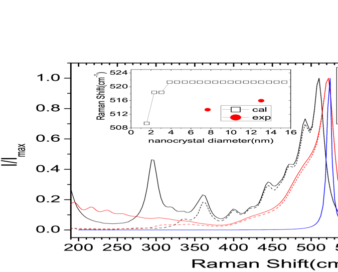
Figure 5: Calculated Raman Shifts vs. nanocrystal diameters with bulk IFCs. The 1.56 nm nanocrystal shows the peak at 509 cm${}^{\text{-1}}$ while the 10.75 nm one at 521 cm${}^{\text{-1}}$. Bulk has a shift of 524 cm${}^{\text{-1}}$. (Inset) The calculated results, shown in square, overestimate the experimental ones, shown in circle.

To demonstrate the redshifts for smaller nanocrystals, we use the bulk IFCs and compare the Raman spectra in Fig 5 for both polarization directions for nanocrystals with diameters 1.56 nm and 10.75 nm along with the bulk which shows the delta-like spectrum with peak at 524 cm${}^{\text{-1}}$. In the inset a clear redshift is shown from 524 cm${}^{\text{-1}}$ down to 509 cm${}^{\text{-1}}$. One observes that the calculated Raman shifts are overestimated ( in the value of 4-7 cm${}^{\text{-1}}$) compared with those from experimentsPRB 73 033307 2006 . There are some aspects in this regard.

The first account for this inconsistency may be that the measured nanocrystals are not uniform in size and we should consider along with the standard deviation of the sizes. But study shows that the standard deviation for 7nm and 13nm cases is roughly 1nm, and in the region the Raman shift barely changes according to the inset in Fig 5. This indicates that even if we consider the size effects of samples due to standard deviation from the production process it will not improve the peak shifts to get closer to the experimental results. Another possible reason may be due to the local heating caused by the laser spot which is roughly 2 or 3 $\mu m$ in diameter and has intensity of several milliWatts on the samplesPRB 80 193410 2009 ${}^{\text{,}}$PRB 66 161311R 2002 local heating . Observable peak shifts are also claimed to be found when tuning the laser to higher power on the same sample. Therefore some studies point out that we may overemphasize the effects of quantum confinements on the peak shift.

III.3.2 The Spectra measured by 488nm Argon-ion Laser

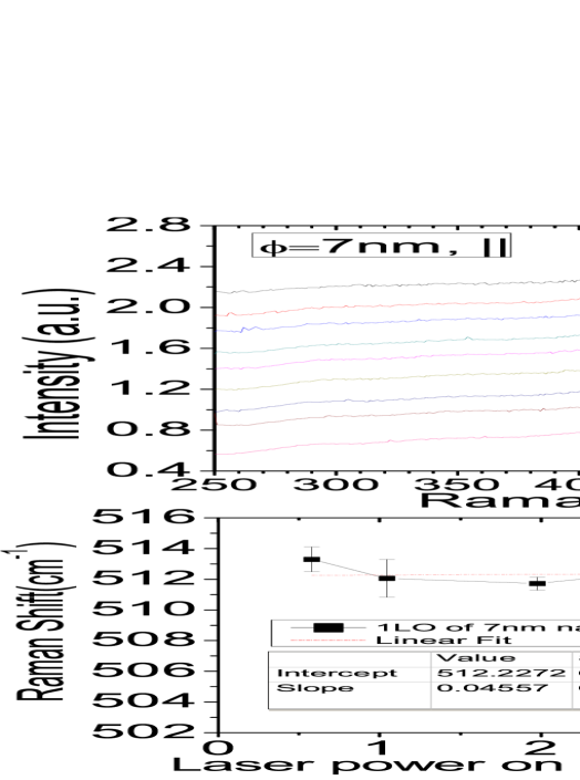
Figure 6: Power variations by 488nm Argon-ion laser on the 7nm case. (A) Raman Spectra under different laser powers on the sample surface. (B) 1LO Raman Shift vs. laser power on the sample surface. No significant shift is observed under different laser powers.

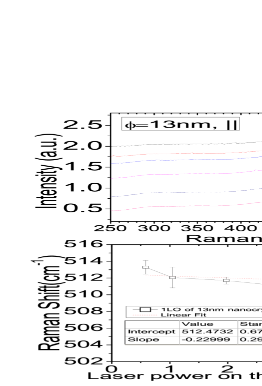
Figure 7: Power variations by 488nm Argon-ion laser on the 13nm case. (A) Raman Spectra under different laser powers on the sample surface. (B)1LO Raman Shift vs. laser power on the sample surface. No significant shift is observed under different laser powers.

In order to investigate this, spectra changes of parallel-polarized scattered light under various incident laser powers in the 7nm and 13nm cases are measured by 488nm Argon-ion laser. To obtain the standard deviation, under each laser power the experiment is repeated 5 times. However, we see that, in Fig 6(B) and Fig 7(B), the 1LO peak shift barely changes under different laser powers. This is contradictory to the studiesPRB 80 193410 2009 ${}^{\text{,}}$PRB 66 161311R 2002 local heating . The studyPRB 80 193410 2009 points out that peak shift influenced by the quantum confinement effect should be negligible for nanocrystals larger than 6 nm, which may be shown by our calculation in the inset of Fig 5 when using bulk IFCs. However, extrapolation in Fig 6(B) and Fig 7(B) shows that under zero laser power the Raman shift should be both around 512 cm${}^{\text{-1}}$ for 7nm and 13nm. Therefore we believe that the quantum confinement still plays the most important role in the redshift (because relaxing the nanocrystal may lead to correct IFCs) for the nanocrystal at least with the size up to 13nm.

Raman peak shifts measured by He-Ne laser for 7nm and 13nm are 513 cm${}^{\text{-1}}$ and 516 cm${}^{\text{-1}}$, respectively. Compared with the zero-power peak shift, 512 cm${}^{\text{-1}}$ for both 7nm and 13nm cases, they are both within the system measuring error. This indicates that the spectra in Fig 3 and Fig 4 by 1.7mW He-Ne laser could be thoroughly ascribed to the quantum confinement effect; the laser local heating may not contribute in the case. In addition, we may infer that the laser local heating may not be very important for the sizes as long as the power is lower than 1.7mW.

III.4 Surface Effects on Some Specific Modes

We now analyze the effects from surface atoms on the three anomalous peaks for the 7nm case observed in Fig 2 but not shown in experiments. For comparisons we also include the effect on the bulk-like peak, 521 cm${}^{\text{-1}}$. To begin with, we study the origin of the four peaks by defining the radial probability distribution $P_{|w-w_{l}|<\Gamma}(r)$ for a certain eigenfrequency $w_{l}$, within a natural broadening $\Gamma$, at the distance $r$ away from the center of the nanocrystal with the radius $R$ as

$$P_{|w-w_{l}|<\Gamma}(r)=\underset{j\in r}{\sum}(\overset{\wedge}{x_{0j}}\cdot\overset{\wedge}{x_{0j}})$$ (22)

, where $\overset{\wedge}{x_{0j}}$ refers to the normalized eigenvector of the atom $j$. Only modes belonging to $A_{1}$, $E$, and $T_{2}$ are summed in a way similar to Eq 21. To see the effects from surface atoms we may calculate the ratio of integrated probability between surface atoms and bulk atoms:

$$\Omega_{w_{l}}=\frac{\int_{r\in S}P_{|w-w_{l}|<\Gamma}(r)dr}{\int_{r\in B}P_{|w-w_{l}|<\Gamma}(r)dr}$$ (23)

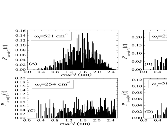
Figure 8: Radial probability distributions for the 7nm case. (A) Bulk-like Raman shift. From (B), (C), and (D) we calculate that the ratios of integrated probability are 40%, 22%, and 33%, respectively. $a=5.43$.

, where $S$ and $\ B$ refer to surface atoms and bulk atoms, respectively. In the case of the 7nm nanocrystals, surface atoms refer to atoms in the range of $r=2.26$ to $r=2.55$. From Fig 8 we obtain $\Omega_{w_{l}=521}=3\%$, $\Omega_{w_{l}=221}=40\%$, $\Omega_{w_{l}=254}=22\%$, and $\Omega_{w_{l}=281}=33\%$. Therefore, surface atoms barely have an effect on the bulk-like 521cm${}^{\text{-1}}$ peak while they may have an effect, at most $40\%$, on the other peaks from single-size contributions. Our samples in reality may be squeezed ellipsoids and this may account for at least $20\%$ why the three modes arising partly from surface atoms may not be shown in experiments. Nonetheless, as discussed above, the most important factor is that the size deviation in real samples smears out the single-size peaks.

IV Conclusions

In conclusions, we first obtain the interatomic force constants up to the second-neighbor atoms, under the rigid-ion model, by directly solving multiple equations that are eigenvalues of the dynamic matrix for bulk Si at the three special points $\Gamma,X,$ and $L$ in the Brillouin zone. The six interatomic force constants (IFCs) thus obtained are compared with the results from ab initio calculations. Besides matching well for the two sets of parameters, we may include as many IFCs for more neighboring atoms as we desire by implementing the results from ab initio calculations. The characteristic vibrations of nanocrystals for free boundary conditions are solved by assuming that the IFCs among atoms in bulk are optimistically applicable

to the atoms in the nanocrystals, with a slight modification of the self energy for surface atoms.

Nanocrystals with sizes of 7nm and 13nm in diameter are produced by thermal evaporations and measured in the backscattering configuration on Raman spectrometer with 632.8nm He-Ne laser and 488nm Argon-ion laser. The polarization of scattered light perpendicular or parallel to that of the incident light is distinguished by using an analyzer in front of the confocal hole. Besides, the first-order Raman spectra are calculated by bond polarizability approximation model. In order to get more satisfactory comparison in the spectrum compared with experiments, the two polarizability parameters are extended up to the second-neighbor atoms. Under this circumstance, asymmetric broadening is seen in fairly good resemblance between calculations and experiments for both sizes measured by the He-Ne laser. Moreover, to investigate the redshifts, various sizes of nanocrystals ranging from 1.56 nm to 15.36 nm are calculated. We see that when using the same IFCs as bulk in the nanocrystals, the peak shifts are almost the same as the diameter of nanocrystals is larger than 4nm; the calculated redshifts overestimate the experimental results at the amount of 4-7 cm${}^{\text{-1}}$, which looks like influenced by the paser local heating effect. But study on laser-power dependence show no significant shifts and therefore it is dubious about the effect of local heating on the redshifts in the Raman Spectrum. We believe that the local heating at most affects the asymmetric broadening on the spectrum shoulders, for higher intensity generates more vibrational modes. However, the peak position should not be influenced. Therefore we infer that the quantum confinement effect plays the major role in the peak shift. Our study shows that we may acquire close peak shift after assigning proper values of IFCs whose change is due to the quantum confinement. For example, in the 7nm case the value $A$ in IFCs changes to $A=-9.56431$, while in the 13nm case, we may set $A=-9.58383$. Extrapolation in the 488nm laser-power dependence shows that both 7nm and 13nm cases have Raman shift around 512 cm${}^{\text{-1}}$ under zero laser power at which the peak shift is totally due to the quantum confinement effect. Compared with the shifts in the He-Ne study, 513 cm^-1 for the 7nm case and 516 cm^-1 for the 13nm case, and noting that each of the two values is within the measuring error of the zero-power shift, 512 cm^-1, it is clear that in the He-Ne study when the laser power is 1.7mW, local heating effect contributes nothing to the redshift.

Finally, the ratios of the integrated probability between surface atoms to bulk atoms show that surface atoms contribute only 3% for the bulk-like mode while they make more contributions, from 20% to 40%, to the other modes originating from nanocrystals in single size.

V
Appendix

Some publicationschang wrong paper 1 ^-chang wrong paper 3 set $E_{1}$ and $E_{2}$ to be zero, however, they did not give any physical explanation. As a matter of fact, one may obtain from the ab initio calculation that neither $E_{1}$ nor $E_{2}$ is zero. Indeed, for some materials $E_{1}$ and $E_{2}$ are zero due to symmetry property. Rocksalt structure, such as NaCl, is an example, but not for the zincblende structure. The problem lies in the wrong arrangement in the short-range part of the dynamic matrix when looking for the three dimensional force-constant matrices other than that of the atom at the position $\frac{a}{4}$($2,2,0$) for which we define in Eq 4. They chose wrong similarity transformation $T_{i}$, resulting in incorrect symmetry in the short-range part of the dynamic matrix. Every element in the dynamic matrix involving $E_{1}$ and $E_{2}$ is wrong. The correct elements involving $E_{1}$ and $E_{2\text{ }}$in the dynamic matrixkunc RIM CPC for calculating zincblende phonon band structure are listed in the row labeled as “correct” in Table II. Terms conjugating to those in Table II are also required to be taken into account. However, in the calculationschang wrong paper 1 ^-chang wrong paper 3 their counterparts are obviously inconsistent. This is due to incorrect assignment for the 3$\times$3 force-constant matrices of the second-nearest atoms.

This mistake seems indifferent for structures with $E_{1}$ and $E_{2}$ to be zero, such as NaCl or MgO. But for materials in the diamond structure, such as Silicon, the mistake may draw to a misleading conclusion that “for Group IV, we must have $E_{1}$ $=$ $E_{2}$ $=0$ to preserve symmetry.” In fact, symmetry property in the diamond structure does not restrict the two terms to be zero. Kunc, et. al.kunc previous , once stated that $E_{1}$ $=$ $E_{2}$ $=0$ when only considering the central-force assumption, but it has nothing to do with symmetry property consideration. Furthermore, there is no reason to take $E_{1}$ $=$ $E_{2}$ $=0$ for materials in zincblende or superlattice, but while setting $E_{1}$ and $E_{2}$ to be nonzero, the lethal mistake will give an unpleasant “bump” near the zone center when exploiting the parametersJ Phys Conden Matt 2 1457 1990 for GaAs, which is shown in Fig. 9 (A).

To avoid the bump, one may mistakenly replace $E_{1}$ and $E_{2}$ to be zero, with the phonon band structure shown in Fig. 9(B). But it does not give the correct structure for optical branches when comparing with the correct ones with appropriate arrangement in the short-range part shown in Fig. 9(C).

However, it raises a very serious question on whether or not their original arrangement in the short-range part produces correct superlattice phonon band structure. Compared with the correct short-range part in the dynamic matrix it is easy to find out that the optical branches of the superlattice in their publications are essentially incorrect, because they did not get correct optical branches for GaAs after assigning E₁ and E₂ to be zero. Therefore, it is imperative to examine again carefully on all of their superlattice-related publications with the rigid-ion model.

Figure 1: Phonon dispersion relation and density of states calculated by Rigid Ion Model with the parameters obtained from solving the multiple equations at the three special points in the first Brillouin zone as well as $E=0.0189$.

Figure 9: GaAs phonon band structure. (A) When setting nonzero E₁ and E₂ in their original fortran procedure, an unpleasant bump is shown near the zone center owing to the wrong symmetry in the short-range part in the dynamic matrix. (B) When assigning the E₁ and E₂ to be zero, the unwanted bump is removed, but we have incorrect optical branches while comparing with the correct band structure in (C).

Table 1: IFCs obtained either by solving Eq. 5 and Eq. 6 with neutron scattering data or by Abinit calculation.

	$A$	$B$	$C$	$F$	$D$	$E$
Neutron Scattering Data	15.69	13.69 12.45 4.51			14.62 12.51 10.97 3.41
Solutions from Eq. 5 and Eq. 6	-9.8315	-6.6725	-0.6373	1.4045	-0.5210	0.0189
Abinit calculations${}^{\text{b}}$	-9.1264	-6.4525	-0.4970	1.1317	-0.4781	0.2944

Table 2: Comparisons between correct and wrong elements involving the parameters E₁ and E₂ in the dynamic matrix for the short-range part.

$DM_{[1,2]}$	correct $-4D_{1}\sin(\pi k_{1})\sin(\pi k_{2})+4iE_{1}\sin(\pi k_{3})\cos(\pi k_{1})-4iE_{1}\sin(\pi k_{3})\cos(\pi k_{2})$ wrong $-4D_{1}\sin(\pi k_{1})\sin(\pi k_{2})+4iE_{1}\sin(\pi k_{1})\cos(\pi k_{3})-4iE_{1}\sin(\pi k_{2})\cos(\pi k_{3})$
$DM_{[1,3]}$	correct $-4D_{1}\sin(\pi k_{1})\sin(\pi k_{3})+4iE_{1}\sin(\pi k_{2})\cos(\pi k_{1})-4iE_{1}\sin(\pi k_{2})\cos(\pi k_{3})$ wrong $-4D_{1}\sin(\pi k_{1})\sin(\pi k_{3})+4iE_{1}\sin(\pi k_{1})\cos(\pi k_{2})-4iE_{1}\sin(\pi k_{3})\cos(\pi k_{2})$
$DM_{[2,3]}$	correct $-4D_{1}\sin(\pi k_{2})\sin(\pi k_{3})+4iE_{1}\sin(\pi k_{1})\cos(\pi k_{2})-4iE_{1}\sin(\pi k_{1})\cos(\pi k_{3})$ wrong $-4D_{1}\sin(\pi k_{2})\sin(\pi k_{3})+4iE_{1}\sin(\pi k_{2})\cos(\pi k_{1})-4iE_{1}\sin(\pi k_{3})\cos(\pi k_{1})$
$DM_{[4,5]}$	correct $-4D_{2}\sin(\pi k_{1})\sin(\pi k_{2})-4iE_{2}\sin(\pi k_{3})\cos(\pi k_{1})+4iE_{2}\sin(\pi k_{3})\cos(\pi k_{2})$ wrong $-4D_{2}\sin(\pi k_{1})\sin(\pi k_{2})+4iE_{2}\sin(\pi k_{1})\cos(\pi k_{3})-4iE_{2}\sin(\pi k_{2})\cos(\pi k_{3})$
$DM_{[4,6]}$	correct $-4D_{2}\sin(\pi k_{1})\sin(\pi k_{3})-4iE_{2}\sin(\pi k_{2})\cos(\pi k_{1})+4iE_{2}\sin(\pi k_{2})\cos(\pi k_{3})$ wrong $-4D_{2}\sin(\pi k_{1})\sin(\pi k_{3})+4iE_{2}\sin(\pi k_{1})\cos(\pi k_{2})-4iE_{2}\sin(\pi k_{3})\cos(\pi k_{2})$
$DM_{[5,6]}$	correct $-4D_{2}\sin(\pi k_{2})\sin(\pi k_{3})-4iE_{2}\sin(\pi k_{1})\cos(\pi k_{2})+4iE_{2}\sin(\pi k_{1})\cos(\pi k_{3})$ wrong $-4D_{2}\sin(\pi k_{2})\sin(\pi k_{3})+4iE_{2}\sin(\pi k_{2})\cos(\pi k_{1})-4iE_{2}\sin(\pi k3)\cos(\pi k1)$

References

- (1) S.-F. Ren, H. Chu, and Y. C. Chang, Phys. Rev. Lett. 59, 1841 (1987).
- (2) S.-F. Ren, H. Chu, and Y.-C. Chang, Phys. Rev. B, 37, 8899 (1988).
- (3) H. Chu, S.-F. Ren, and Y. C. Chang, Phys. Rev. B 37, 10746 (1988).
- (4) K. Kunc and O. Holm Nielsen, Computer Phys. Commu. 16, 181 (1979).
- (5) K. Kunc, M. Balkanski, and M. A. Nusimovici, Phys. Stat. Sol. (b) 71, 341 (1975).
- (6) D. Strauch and B. Dorner, J. Phys.: Condens. Matter 2, 1457 (1990).