Collective excitations and low temperature transport properties of bismuth

Abstract

We examine the influence of collective excitations on the transport properties (resistivity, magneto-optical conductivity) for semimetals, focussing on the case of bismuth. We show, using an RPA approximation, that the properties of the system are drastically affected by the presence of an acoustic plasmon mode, consequence of the presence of two types of carriers (electrons and holes) in this system. We find a crossover temperature $T^{*}$ separating two different regimes of transport. At high temperatures $T>T^{*}$ we show that Baber scattering explains quantitatively the DC resistivity experiments, while at low temperatures $T<T^{*}$ interactions of the carriers with this collective mode lead to a $T^{5}$ behavior of the resistivity. We examine other consequences of the presence of this mode, and in particular predict a two plasmon edge feature in the magneto-optical conductivity. We compare our results with the experimental findings on bismuth. We discuss the limitations and extensions of our results beyond the RPA approximation, and examine the case of other semimetals such as graphite or $1T-TiSe_{2}$.

I Introduction

Bismuth is a material which plays an important role in solid state physics. Due to an extremely small Fermi surface this material provides the remarkable possibility to observe strong effects induced by the presence of external fields, pressure and temperature, even if these external forces are of moderate amplitude. Several important phenomena, Shubnikov-de Haas[1] and de Haas-van Alphen[2] effects, were observed for the first time in bismuth. In a last few years a series of experiments have once again drawn the attention of the community to elemental bismuth, and challenged our understanding of this material. High pressure optical spectroscopy measurements indicate that the mechanism of semimetal to semiconductor decay is not fully understood[3]. Reflectivity measurements[4] showed large changes in the plasmon frequency and anomalous mid-infrared features, indicating strong scattering of the electronic degrees of freedom by a plasmon collective mode. An extremely strong Nernst signal with unusual temperature dependence (both at low[5] and high fields[6, 7]) was also reported.

These recent experiments were showing clearly that the question of transport in bismuth was still not understood. In fact similar questions still existed for the standard resistivity as well. The majority of the resistivity experiments had been done in late 70s, beginning with the works of Hartmann[8], Kukkonen[9] and later studies[10], who showed that down to 4K the Fermi liquid theory (with components of very different masses) works quite well. The $T^{2}$ resistivity behavior at lowest temperatures was explained within this theory[11, 9]. However the discussion was not closed because one year later more detailed, lower temperature data by Uher[12] was published, and showed a significant deviation from expectations: the $T^{2}$ behavior changes smoothly into a $T^{5}$ behavior at the lowest temperatures. A quite complex theory involving coupling to particular group of phonons was proposed as an explanation of this result[13].

The purpose of this work is to re-examine the theory of transport in semimetals. We show that these anomalous transport properties have a simple explanation. They come from the fact that the coupling between electrons and holes with very different masses induces many body corrections to the Fermi liquid picture. In fact the above mentioned change in the resistivity was the first example how interactions in semimetals modify the simple Fermi liquid picture. Although our study is mostly focused on bismuth, we also examine other materials which have been recently the subject of intensive studies, such as graphite[14, 15] and $1T-TiSe_{2}$[16, 17].

The structure of this paper is as follows. In Sec. II we introduce the model of interaction between the electrons and holes. We show that at low temperatures, a collective acoustic plasmon mode exists and plays a central role in the properties of the material. We discuss also the high temperature regime of conductivity and show that the Baber mechanism[18] is the dominant source of resistivity in this regime. We then examine in Sec. III the low temperature regime for the resistivity. We develop an effective theory for this regime and derive a new $\rho(T)$ dependence, which is a direct consequence of the existence of a collective acoustic plasmon mode. We examine the magneto-transport in Sec. IV. We show in particular that a double plasma edge must exist. Some discussion on the validity of the approximations used to derive the above mentioned results are indicated in Sec. V and conclusions in Sec. VI. Some technical details can be found in the appendices.

II Mechanism of resistivity

II.1 Band structure and hamiltonian

The peculiarity of bismuth comes from the very small characteristic energy scales of its Fermi liquid (see Fig. 1).

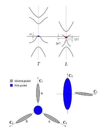
Figure 1: A sketch of the band structure of bismuth: three electron pockets and a central hole pocket. (top) the energy dispersion. Energies are in meV. (bottom) The four pockets. The scale is grossly exaggerated. In fact $k_{F}$ are $10^{4}$ smaller than intra-pocket distances. The electron pockets are slightly tilted out of bisectrix-binary plane $C_{1}-C_{2}$ perpendicular to the trigonal axis $C_{3}$. Figure after Ref.20

This stems from a slightly distorted cubic crystal structure (the distortion angle is smaller than $3^{\circ}$). In the absence of distortion bismuth would be a band insulator, instead it is a quite rare rhombohedral space group $A7$ (without inversion symmetry). Bismuth becomes a semimetal with very small amounts of fermions active at accessible energies.

The hamiltonian of those carriers close to Fermi energy in bismuth reads in general:

$$H=H_{0}^{h}+\sum_{\nu=1}^{3}H_{0}^{e\nu}+H_{int}^{h-h}+H_{int}^{e-e}+H_{int}^{e-h}$$ (1)

In the above $h$ denotes a hole pocket, while there are three electron pockets denoted by $e\nu$. The first two terms are the free fermion kinetic energies. We approximate the kinetic energy of each type of carrier by a a free dispersion relation

$$\xi^{\alpha}(k)=\sum_{i=1}^{3}\frac{\hbar^{2}k_{i}^{2}}{2m_{i}^{\alpha}}-E_{F}^{\alpha}$$ (2)

where $\alpha$ denotes the species, the index $i$ are the three principal axes of the energy ellipsoid (see Fig. 1), $m_{i}^{\alpha}$ is the mass tensor, the $k$ are the momenta centered on the corresponding pocket and $E_{F}^{\alpha}$ the Fermi energy of the corresponding species. The values of the parameters are summarized in Table 1.

	$m_{1}$	$k_{F1}$	$m_{2}$	$k_{F2}$	$m_{3}$	$k_{F3}$
holes	0.067	0.01	0.067	0.01	0.612	0.03
electrons	0.198	0.06	0.0015	0.005	0.0021	0.005

Table 1: The band parameters of bismuth according to Ref. 19. Masses are in units of the mass of the electron, and wavevectors in units of reciprocal length $1.386\AA^{-1}$. The values are given along the principal axes of the ellipsoids as defined in Fig. 1.

We want to emphasize that this peculiar band structure was computed quite accurately and this result was later confirmed by many experimental probes.

The latter terms in (1) are interactions, whose influence is the subject of this study. We divided interactions into three groups: hole-hole, electron-electron and electron-hole. Each one of these terms has the form

$$H_{int}^{\alpha-\beta}=\sum_{q}V^{\alpha\beta}(q)\rho_{\alpha}(q)\rho_{\beta}(-q)$$ (3)

where $\alpha,\beta$ runs among the species. The density operators $\rho_{\alpha}(q)$ is given by

$$\rho_{\alpha}(q)=\sum_{k}c^{\dagger}_{\alpha,k+q}c_{\alpha,k}$$ (4)

where the $c^{\dagger},c$ are the standard fermionic creation and destruction operators and a summation overs the spin degrees of freedom is implicit. The interaction potential is the long-range Coulomb potential

$$V^{\alpha\beta}_{\rm coul}(q)=\frac{e_{\alpha}e_{\beta}}{\epsilon_{\infty}q^{2}}$$ (5)

where the hole charge is the opposite of the electronic one $e_{h}=-e_{e}$ and $\epsilon_{\infty}$ is the dielectric constant due to the rest of the material. Because of the very small size of the pockets and the large distance in momentum space among them all interactions which implies a transfer of particle from one pocket to the other must occur with a large momentum transfer. These terms are thus potentially strongly suppressed compared to the intra-pocket interactions given the long-range nature of the Coulomb potential (5).

II.2 Screened Coulomb interaction: acoustic plasmon

The smallness of the bismuth Fermi surface shown in Fig.1 and incorporated in the first two terms of the hamiltonian (1) has certain non-trivial implications for the transport properties. When $k_{F}^{-1}\approx 10^{4}\AA$ the interaction with angstrom size impurities is strongly reduced. The probability of intra-pocket umklapp scattering is also very low. Since the Debye temperature for Bi is around $150K$ it implies that at $T\sim 1K$ phonon influence will be rather weak. Moreover thermal transport is proven experimentally to be ballistic. No evidence of any additional order parameter, generating quasi-particles on which carriers could scatter was found in the many decades of careful studies of this element. Thus in order to understand the transport properties we can restrict ourselves to the Fermi liquid part of the problem described by the hamiltonian (1).

Given the above points, the main type of scattering entering resistivity should be the so-called Baber scattering[18], coming from the presence of several types of carrier of different masses. In contrast with all the above mentioned scattering processes Baber scattering is strongly favored by the band structure of Bi – the ratio of electrons and holes masses being in some directions more than a factor of $10$. The resistivity in Bismuth is thus linked directly to the electron-hole interaction term in (1).

Although the bare form of such a term is given by (3), the presence of the two species of carriers leads to a strong renormalization of the bare Coulomb interaction due to dynamical screening. We thus need to examine the effects of screening on the interaction potential $V^{\alpha\beta}(q)$. Normally we have a tensor structure for the screened interaction (or alternatively the dielectric constant), but if we assume that the longitudinal and transverse modes do not mix, which is a good approximation in Bismuth, then we can use the standard Random Phase Approximation (RPA) for the Coulomb potential. In the presence of two types of carrier the RPA equations are indicated in Fig. 2.

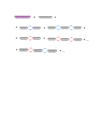
Figure 2: The RPA series for effective interactions for the case of a two component system. We denote generically these components by $r$ (rapid or fast) and $s$ (slow). In the above diagram, the thick coil is the screened effective interaction $V_{\rm eff}(q,\omega)$, the solid blue denotes using the standard diagrammatic convention a fast particle, while the doted red line is a slow particle. The black coil is the bare Coulomb potential (5).

The equation of Fig. 2 can be solved doing first the re-summation on one of the species:

$$\tilde{V}^{ee}(q,\omega)=\frac{V^{ee}_{\rm coul}(q)}{1-V^{ee}_{\rm coul}(q)\Pi_{hh}(q,\omega)}$$ (6)

where $\Pi_{hh}(q,\omega)$ is the retarded density-density correlation function for the holes, including the interactions which are not already present in the RPA chain of bubbles of Fig. 2. The simplest and usual approximation for $\Pi_{hh}$ consists in taking the free correlation $\Pi^{0}_{hh}(q,\omega)$. Using the Hamiltonian (1) one has

$$\Pi^{0}_{hh}(q,\omega)=\frac{1}{\Omega}\sum_{k}\frac{f(\xi(k))-f(\xi(k+q))}{\omega+\xi(k)-\xi(k+q)+i\delta}$$ (7)

where $\Omega$ is the volume of the system, $f$ the Fermi factors, $\delta=0^{+}$. Using this expression one can get the screening of the electron-electron potential

$$V_{\rm eff}^{ee}(q,\omega)=\frac{\tilde{V}^{ee}(q)}{1-\tilde{V}^{ee}(q,\omega)\Pi_{ee}(q,\omega)}$$ (8)

where $\Pi_{ee}(q,\omega)$ denotes the sum over the three electron pockets of the corresponding retarded density-density correlation $\Pi_{ee}(q,\omega)=\sum_{\nu=1}^{3}\Pi_{ee,\nu}(q,\omega)$. The expression (8) can be rewritten as

$$V_{\rm eff}^{ee}(q,\omega)=\frac{V^{ee}_{\rm coul}(q)}{1-V^{ee}_{\rm coul}(q)[\Pi_{hh}(q,\omega)+\Pi_{ee}(q,\omega)]}$$ (9)

where in a similar way than for the holes one can approximate the correlation function by its free (or Fermi liquid) value.

As can be seen from (9) a strong resonance in $V_{\rm eff}^{ee}(q,\omega)$ exists when the denominator is small, which indicated the presence of a collective mode. As usual the dispersion relation of the mode is given by

$$1=V^{ee}_{\rm coul}(q){\rm Re}[\Pi_{hh}(q,\omega)+\Pi_{ee}(q,\omega)]$$ (10)

where ${\rm Re}$ denotes the real part. The imaginary part gives the damping of the mode. As is well known[21, 22, 23] for the case of a two component system (10) has two solutions. One is the standard optical plasmon, but a second one is an acoustic mode

$$\omega_{ac}=uq=(c_{\rm ac}-\imath\tau^{-1})q$$

where $Re[u]=u^{\prime}=c_{\rm ac}$ is the acoustic plasmon velocity and $Im[u]=u^{\prime\prime}=-\tau^{-1}$ the damping of the mode. For the case of isotropic Fermi surfaces with the same Fermi wavevector for the two species (neutrality condition) and one heavy $m_{s}$ and light masses $m_{r}$ (for slow and rapid carriers respectively) such that $(V_{Fs}/V_{Fr})^{2}\ll 1\ll m_{s}/m_{r}$, where the $V_{Fi}$ ($i=r,s$) are the respective Fermi velocities $k_{Fi}/m_{i}$ with $E_{F}^{i}=k_{Fi}^{2}/(2m_{i})$ in the zeroth order approximation (extreme mass difference), one has

$$c_{\rm ac}^{0}=\sqrt{V_{Fr}V_{Fs}/3}$$ (11)

and

$$(\tau^{0})^{-1}=\pi V_{Fs}/12$$ (12)

Physically such an acoustic plasmon comes from the fact that for two different velocities, one of the species (the light one) will have a much larger Fermi velocity than the acoustic plasmon mode. In that case the corresponding $\Pi_{rr}(q,\omega)$ essentially tends to a constant $\Pi_{rr}(q\to 0,\omega=0)$ which is the density of states at the Fermi level. This mode is fast enough to screen the Coulomb interaction. (6) would just become

$$\tilde{V}^{rr}(\omega=c_{\rm ac}q\to 0)=\frac{1}{-\Pi_{rr}(\omega=c_{\rm ac}q\to 0)}$$ (13)

transforming the original long range interaction into a short range one. Using the well known result for the Lindhard function one gets

$$-\Pi_{rr}(\omega=c_{\rm ac}q\to 0)=\frac{m_{r}k_{Fr}}{\pi^{2}}+\imath\frac{m_{r}^{2}c_{\rm ac}}{2\pi}$$ (14)

For the heavy mode one is in the opposite limit $c_{\rm ac}\gg V_{Fs}$ for which the Lindhard function is approximately

$$-\Pi_{ss}(\omega=c_{\rm ac}q\to 0)=\frac{m_{s}k_{Fs}}{\pi^{2}}\frac{k_{Fs}^{2}}{3c_{\rm ac}^{2}m_{s}^{2}}$$ (15)

Substituting (13) into (8) one gets the results (11) and (12).

Such collective excitation has been already investigated in several systems [21, 22, 24] but is normally very elusive. It exists usually very close to the single-particle excitation spectrum, so it can be easily Landau overdamped. There were proposals[25] suggesting its measurability in artificial 1D systems (quantum wires), but even then its intensity was shown to be much weaker than optical plasmon and was easily suppressed by disorder. However we claim in the present paper that such a collective mode plays an important role in Bismuth. Computing precisely its parameter is a singularly complicated calculation given the complexity of the Fermi surface and the presence of the various masses. Nevertheless we give in Appendix A arguments for the existence of such a mode. Mostly we will proceed along the lines that such a mode exists and explore the consequences for the various transport properties.

Note that the mode never exists as a perfectly sharp mode, because of the damping (12) which always gives a finite width of the order of $\tau^{-1}$ to this acoustic plasmon resonance. In addition the mode will completely disappear when its dispersion relation will enter the the particle-hole continuum of excitations of the heavy (slow) species. Beyond this point the mode is severely damped and does not exist as a collective excitation anymore. The corresponding wavevector $q^{*}$ can be determined by matching the energy of the acoustic plasmon $\omega=c_{\rm ac}q$, taking into account a width of order $\tau^{-1}q$ with the edge of the particle-hole spectrum $q(q+2k_{Fh})/2m_{h}$. An estimate of this wavevector is thus

$$q^{*}\simeq 2m_{h}[c_{\rm ac}-V_{Fh}-\tau^{-1}]$$ (16)

This condition which is essentially similar to the one for $k_{c}$ in Ref. 24 (where $V_{Fs}q$ and $2k_{Fs}$ were taken as energy and momentum units).

Correspondingly $q^{*}$ defines an energy and temperature scale

$$T^{*}\sim c_{\rm ac}q^{*}$$ (17)

This temperature play a similar role than the Debye temperature for acoustic phonons: there are no bosonic states to be occupied beyond. On the other hand below this temperature the physics of the system is affected by the existence of the extra collective mode – there are plasmon states whose occupation fluctuations can affect carriers mobilities. Based on the above we see that we can potentially distinguish two very different temperature regimes:

$T>T^{*}$

This is the high temperature (HT) regime. In that regime there is no collective mode and we can treat Bismuth as a double Fermi liquid. We can thus deal with the electron-hole scattering in the usual way, for example by solving the Boltzman transport equation, or equivalent approximations. We will briefly discuss this rather conventional regime in Sec. II.3.

$T<T^{*}$

This is the low temperature (LT) regime. In that regime, the presence of the acoustic plasmon plays a central role in the interactions among particle. It will thus affect strongly the scattering between electrons and holes and lead to very different transport properties. The study of the consequences of such a mode is at the heart of the present paper and will be done for the resistivity in Sec. III and in the subsequent sections for other transport coefficients.

II.3 High temperature regime: Baber resistivity

Let us now examine the resistivity itself. As discussed above we have to distinguish two different regimes of temperature. We examine in this section the high temperature one, which shows relatively conventional transport properties, and will concentrate on the low temperature regime in the next section.

At high temperature no collective mode is present and thus we have two well defined Fermi liquids. The resistivity is coming from the electron-hole interaction since this is the only term that does not conserve the total current. Indeed given the quadratic dispersion relation the current is proportional to the momentum and thus the intra-species interactions conserve the total current. The main source of resistivity is this regime is the Baber scattering[11], which leads within a standard Boltzmann approximation to

$$\rho=(\frac{m_{e}m_{h}k_{B}}{3\pi e\hbar^{3}\sqrt{n}})^{2}WT^{2}=AT^{2}$$ (18)

where $W$ is the e-h scattering rate and $n$ the density of particles of a given species. This gives an approximation for the coefficient $A$ of the $T^{2}$ term in the resistivity $\rho=AT^{2}$, which is usually the quantity extracted from experimental data. Thus, provided that one is able to compute $W$, we have a parameter free fit for experiment. The prefactor $W$ was computed using a Thomas-Fermi approximation for the Coulomb interaction[11] leading to

$$W=\frac{2\pi}{\hbar}\int_{0}^{2k_{Fs}}\frac{dq}{2k_{Fs}}V_{\rm TF}(q)^{2}[3(q/2k_{Fs})^{2}]$$ (19)

where $k_{Fs}$ is the Fermi wavevector of the slower component. $V_{\rm TF}(q)$ is the Thomas-Fermi screened Coulomb interaction:

$$V_{eff}(q)=\frac{4\pi e^{2}}{\epsilon_{\infty}q^{2}+\kappa_{T-F}^{e2}+\kappa_{T-F}^{h2}}$$ (20)

Ref. 11 estimated the above terms using $\epsilon_{\infty}=100$, $\kappa_{T-F}^{i}=3(4m_{i}^{2}k_{Fi}/\pi\hbar^{2})$where $m_{e}=0.03$, $m_{h}=0.15$ which were known from previous independent measurements. This led to $A=8n\Omega cmK^{-2}$ in good agreement with the experimental data of that time $8n\Omega cmK^{-2}$ (the first reported in Ref.26), $14.5n\Omega cmK^{-2}$ (in Ref.8) and also the more recent ones[12, 6] $12n\Omega cmK^{-2}$ for measurements along the binary axis. With the same formulas an even better value $A=14n\Omega cmK^{-2}$ can be found if we use more recent values of parameters: $\epsilon_{\infty}=88$, $m_{e}=0.04$, $m_{h}=0.14$. The $Bi_{1-x}Sb_{x}$ compound, with $x=0.037$ ($n_{x=0.037}\approx n_{x=0}/3$) was also measured[7] and the experimental $A=33n\Omega cmK^{-2}$, is in agreement with the expectations from (18), showing that the Baber scattering is indeed the good description of the the transport in this regime of parameters. However low temperature deviation from this simplistic picture were reported already in early works (see Ref.9 and a detail discussion there)

Within the framework of the Baber scattering, one can go beyond the traditional Baber formula (18) in two ways. First the large temperature behavior can be computed as well[27]. At high enough temperature the $T^{2}$ behavior of (18) crosses over, at a temperature of the order of $T_{l}\sim 0.2\sqrt{T_{Fe}T_{Fh}}$ to a linear temperature dependence. Experimental data in Bismuth shows indeed above $T=3K$ a clear $T^{2}$ dependence, becoming linear above $T=25K$. This is in reasonable agreement with the estimate given by the above formula which for Bismuth would be $T_{1}\sim 35K$. Second, one can refine the calculation of the coefficient $A$ by taking into account the ellipsoidal character of the Fermi surface, rather than using the best fit for spherical Fermi surface approximation ($m_{e}=0.04$, $m_{h}=0.14$). The procedure is given in Appendix B for the simplified case of two pockets only. The ratio of resistivities in different directions $x$ and $z$ is proportional to:

$$\frac{\rho_{x}}{\rho_{z}}=\left[\frac{|m_{ex}-m_{hx}|/(m_{ex}+m_{hx})}{|m_{ez}-m_{hz}|/(m_{ez}+m_{hz})}\right]^{2}$$ (21)

Given the masses of Table 1 we expect that resistivity will be largest along the trigonal axis of the crystal. The value of the asymmetry $\approx 1.4$ that the above formula gives is slightly larger than the experimentally[8] found one $\approx 1.15$. However one has to remember that due to highly anisotropic ellipsoids constituting the Fermi surface the experiment requires a very precise monocrystal orientation.

However the Baber scattering does not allow to understand the low temperature regime which in Bismuth corresponds to $T<3K$. For this regime one has to invoke the existence of the acoustic plasmon. This is the regime that we consider now.

III Low temperature regime

III.1 Effective hamiltonian for lowest temperatures

As we determined in the previous section, at low enough temperature an acoustic plasmon mode exists. The very existence of this mode implies that for some values of the frequency and momenta the effective interaction $V_{\rm eff}(q,\omega)$ between the carriers will have a pole. One can thus expect this pole to dominate the low temperature transport.

In order to analyze the consequences of such a pole, we derive an effective low energy Hamiltonian for which we consider this collective mode as a particle. This can be done by replacing the term corresponding to $V_{\rm eff}(q,\omega)$ (as shown in Fig. 3) by the propagator of a particle, representing the bosonic fluctuations of the plasma and ensuring that terms such as the self-energy terms such as the ones of Fig. 3 are correctly reproduced. Such a model is given by the coupling of electrons and holes to phonon-like excitations

$$H=H_{0}^{h}+H_{0}^{e}+\sum_{q}\omega_{q}b^{\dagger}_{q}b_{q}+\frac{1}{\sqrt{\Omega}}\sum_{\alpha=e,h}\sum_{q}M_{q}^{\alpha}[b^{\dagger}_{-q}+b_{q}]\rho_{\alpha}(q)$$ (22)

with such an Hamiltonian the electron self energy of Fig. 3 would be

$$\Sigma_{e}(q,i\nu_{n})=-\frac{1}{\beta\Omega}\sum_{\omega_{n},q}(M_{q}^{e})^{2}D(q,i\omega_{n})\frac{1}{i\nu_{n}+i\omega_{n}-\xi_{e}(k+q)}$$ (23)

where the $\nu_{n}$ and $\omega_{n}$ are the usual Matsubara frequencies and $D(q,i\omega_{n})$ is the phonon propagator

$$D(q,i\omega_{n})=-\frac{2\omega_{q}}{\omega_{n}^{2}+\omega_{q}^{2}}$$ (24)

The corresponding term for the original Hamiltonian is shown in Fig. 3 and is given by

$$\Sigma_{e}(q,i\nu_{n})=-\frac{1}{\beta\Omega}\sum_{\omega_{n},q}V_{\rm eff}(q,i\omega_{n})\frac{1}{i\nu_{n}+i\omega_{n}-\xi_{e}(k+q)}$$ (25)

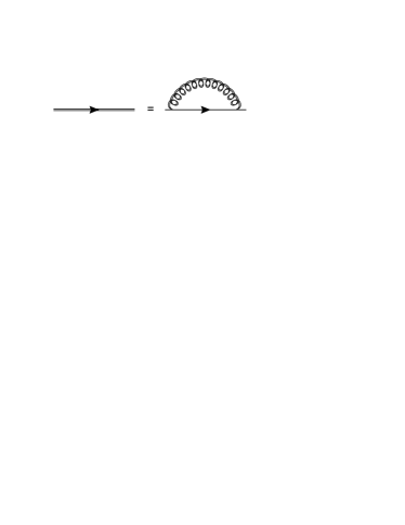
Figure 3: a) The self-energy of a fermion (an electron or hole) experiencing $V_{eff}(q,\omega)$ interaction (a double coil as in Fig. 2) during its propagation; as explained in the text the effective interaction $V_{eff}(q,\omega)$ is of the resonance form.

One can show on this term, and the other diagrams, that the expansion is essentially identical provided one identify the proper “phonon” propagator and interaction vertex $M_{q}$. This can easily be done on the spectral function $A(q,\omega)=-\frac{1}{\pi}{\rm Im}D(q,i\omega_{n}\to\omega+i\delta)$. We only consider $\omega>0$ since $\omega<0$ can easily be deduced from it. The “phonon” spectral function is

$$A_{\rm ph}(q,\omega>0)=\delta(\omega-\omega_{q})$$ (26)

The effective potential $V_{\rm eff}(q,\omega)$ of (9) is more difficult to evaluate fully. However using the simple case of two types of particles (fast and slow) as discussed in the Sec. II.2 one has

$$V_{eff}(q,\omega)=\left(\frac{3\pi^{2}m_{r}}{k_{Fr}^{3}}\right)\frac{1}{c_{\rm ac}^{2}}{1-c_{\rm ac}^{2}q^{2}/\omega^{2}+\imath\pi c_{\rm ac}/2}$$ (27)

There is a finite lifetime due to the imaginary part (12), leading to a lorentzian spectral function. If for the moment we ignore this finite width and assimilate the resonance to a $\delta$-function peak we have for the spectral function

$$A_{\rm plasmon}(q,\omega>0)=\left(\frac{3\pi^{2}m_{r}}{k_{Fr}^{3}}\right)\frac{c_{\rm ac}^{3}|q|}{2}\delta(\omega-c_{\rm ac}|q|)$$ (28)

One can thus directly identify the two processes with

$$\begin{split}\omega_{q}&=c_{\rm ac}|q|\\ M_{q}^{e0}&=\left(\frac{3\pi^{2}m_{r}c_{\rm ac}^{3}}{2k_{Fr}^{3}}\right)^{1/2}|q|^{1/2}\end{split}$$ (29)

where $M_{q}^{e0}$ is the zeroth order approximation for the strength of electron-plasmon interaction (as introduced in Eq. 22). The above identification allows us to replace the problem of the screened Coulomb potential, by a problem of electrons and holes interacting with a bosonic particle. Of course this particle represents the quantization of the acoustic plasmon.

Let us make some comments on the validity of the identification (29). Of course the real calculation of the term $V_{eff}(q,\omega)$ or $M_{q}^{e}$, specially at finite temperature would be more complex, and will certainly affect the quantitative aspects of the identification. However we expect the qualitative features of the mode identification to be robust. In particular the frequency of the acoustic plasmon will of course be linear in $u\sim q$ at small $q$, and in the same way the matrix element describing the coupling to the particles will go as $M_{q}^{e}\sim q^{1/2}$. Note that this specific dependence of the coupling constant is what makes the difference between the coupling to this acoustic plasma mode and the coupling to normal acoustic phonons. This will have of course consequences for the temperature dependence of the resistivity that we will explore in the next section. The most drastic approximation that we made was to ignore the finite lifetime of the mode and to concentrate the full spectral weight in a $\delta$-function peak. This approximation is not essential, and the finite lifetime can of course be taken into account. It would simply correspond to a damping of the phonon mode. It simplifies however the subsequent calculations and allows to extract the physics in a more transparent way so we stick to it in the reminder of this paper. On a quantitative level, both the broadening of the level $u^{\prime\prime}q$ and the average energy $u^{\prime}q$ are proportional to $q$, as discussed in the previous section. For Bismuth a typical order of the ratio $u^{\prime\prime}/u^{\prime}$ is $u^{\prime\prime}/u^{\prime}\approx 0.25$ so we expect such an approximation to be reasonably quantitative as well.

We can now use the standard diagrammatic analysis of electron-phonon interaction, keeping in mind the difference in the matrix elements, to obtain the various physical quantities when the acoustic plasmon is playing a major role. In particular the self energy (23) is simply given, after summation on the Matsubara frequencies by

$$\Sigma_{e}(q,i\nu_{n})=\frac{1}{\Omega}\sum_{q}(M_{q}^{e})^{2}[\frac{b(\omega_{q})+f(\xi(k+q))}{i\nu_{n}+\omega_{q}-\xi(k+q)}-\\ \frac{b(-\omega_{q})+f(\xi(k+q))}{i\nu_{n}-\omega_{q}-\xi(k+q)}]$$ (30)

Since we are interested in the low energy dissipation we perform the analytical continuation $i\nu_{n}\rightarrow\nu+\imath\delta_{+}$, then the limit $\nu\rightarrow 0$ and finally extract the imaginary part of $\Sigma_{e}$. This last step leads to a delta function constraints implementing the energy conservation (see e.g. (40)). This equation gives us a 2D surface $\Omega_{0}$ of solutions $q_{0}$ for $q$. However the above sum on $q$ in (30) should be limited to the values for which the acoustic plasmon exists. We should thus only look at values of $q$ lower than $q^{*}$ which was defined in (16). For small angles only one of the masses dominates (63). Combining this with (11) and the fact that we work in $\omega\rightarrow 0$ limit, we deduce that in a limit of small angles (nearby direction of high symmetry) $c_{ac}(\theta)\sim\cos(\theta)$ which implies $q_{0}(\theta)=q^{*}\cos(\theta)$. One has thus always $q_{0}(\theta)\leq q^{*}$. Although potentially this criterion can depend on the direction of $q$, based on above considerations, we can assume here that the directions of $\vec{q}$ where $q^{*}(\theta)$ drops to extraordinarily small values are rare. In particular this means that the surface $\Omega_{0}$ is well defined. To obtain numerical responses we will take an isotropic criterion for the upper cutoff.

III.2 New $\rho(T)$ dependence

In the low temperature regime, the transport of the system, which is now dominated by the presence of the acoustic plasmon, can thus be described by the effective Hamiltonian (22). One has of course to keep in mind that because of the unusual $q$ dependence of the coupling to this bosonic degree of freedom (29) the temperature dependence of the resistivity will not be the one of the usual electron-phonon problem.

To compute the resistivity we use the Kubo formula and express the resistivity as the current-current correlation function

$$Re[\sigma_{xx}(\omega\rightarrow 0)]=\\ lim_{\omega\rightarrow 0}\frac{ne^{2}}{\omega}Im[\langle j_{x}(Q=0,\omega)j_{x}(-Q=0,0)\rangle]$$ (31)

We are interested in the uniform response, so we set $Q=0$, we will omit $x$ index in the following. The current is simply given by

$$J=\sum_{k,\alpha}e_{\alpha}\frac{k_{x}}{m_{x\alpha}}c^{\dagger}_{k\alpha}c_{k\alpha}$$ (32)

where $\alpha$ is the particle species, $e_{\alpha}$ and $m_{x\alpha}$ the corresponding charge and mass in the direction of movement. The corresponding diagram is shown on Fig. 4a where the thick line and shaded triangle indicate that both propagator and interaction vertex are renormalized by $V_{eff}(q,\omega)$). The average in (31) will be computed with the effective hamiltonian of the problem given by (22). It is important to note that given the topology of the diagrams entering the vertex corrections there is indeed no double counting of diagrams if one replaces the thick coil of Fig. 4 by the bosonic excitation as done in (22).

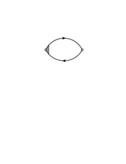
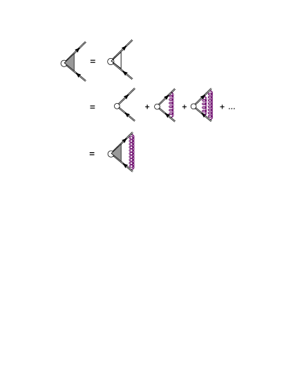
Figure 4: a) The diagrammatic form of current-current correlation function. The double line is the full Green’s function for the electrons or holes while the shaded box denotes the vertex correction which is shown in part b). In b) the ladder series for vertex correction is shown. The irreducible part consist on single plasmon exchange (purple coil line) between the fermions (electrons or holes). As for normal phonons given the momentum dependence of the coupling constant $M_{q}$ and propagator, it is crucial to include the vertex correction to get the proper temperature dependence.

The procedure is standard[28], and follows closely the one for phonons. The vertex correction makes it cumbersome, so we give here a derivation based on the memory function that has the advantage to take directly the vertex correction into account in a simpler way. The conductivity can be expressed as

$$\sigma(\omega)=\frac{i\chi_{0}}{\omega+M(\omega)}$$ (33)

where $\chi_{0}$ is the diamagnetic term, and $M(\omega)$ is defined as:

$$M(\omega)=\frac{\langle F;F\rangle_{\omega}-\langle F;F\rangle_{0}}{-\chi(0)\omega}$$ (34)

where the force $F$ is $F=[j,H]$, and the $\langle F;F\rangle_{\omega}$ denotes the standard retarded correlation function at frequency $\omega$. The averages are computed with the the part of the Hamiltonian that commutes with the current. Given that $M=0$ if the current commutes with $H$ one recovers immediately in that case from (33) that the system is a perfect conductor. In particular in the high temperature regime it shows immediately that the sole source of resistivity is the electron-hole interaction and the difference of masses between the two species.

For low temperatures, in the case of the Hamiltonian (22), and using the definition of the current (32) one obtains for $F$ (for simplicity we only kept two species $e$ and $h$)

$$F=\sum_{q,k,\alpha}e_{\alpha}M_{q\alpha}\frac{q_{x}}{m_{\alpha}}c^{\dagger}_{k+q,\alpha}c_{k,\alpha}[b^{\dagger}_{-q}+b_{q}]$$ (35)

Each species gives thus a contribution to F-F correlation which is shown on Fig.  and for Matsubara frequencies equals to:

$$\langle F;F\rangle_{\omega_{n}}=\frac{1}{\beta^{2}\Omega^{2}}\sum_{\nu_{1},\nu_{2},k,q}\frac{M_{q}^{2}q_{x}^{2}}{m^{2}}G(\nu_{1},k)G(\nu_{2},k+q)\\ D(\omega_{n}+\nu_{1}-\nu_{2},q)$$ (36)

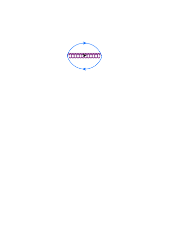
Figure 5: The force-force (F-F) correlation diagram. The solid blue line indicates propagator of fermion (one, for example slower, component of the Fermi liquid) while the purple coil is the plasmon propagator

The frequency summation can be performed which gives

$$\langle F;F\rangle_{\omega_{n}}=\frac{1}{\Omega^{2}}\sum_{k,q}\frac{M_{q}^{2}q_{x}^{2}}{m^{2}}\\ \frac{[f(\xi(k+q))+b(-\omega_{q})][f(\xi(k)-f(\xi(k+q)+\omega_{q})]}{i\omega_{n}+\xi(k)-\xi(k+q)-\omega_{q}}\\ -(\omega_{q}\to-\omega_{q})$$ (37)

After the analytic continuation one gets for the imaginary part of the function $M(\omega)$

$${\rm Im}M(\omega\to 0)=\frac{\pi}{\Omega^{2}}\sum_{k,q}\frac{M_{q}^{2}q_{x}^{2}}{m^{2}}\frac{\partial f}{\partial\xi(k)}[f(\xi(k+q))+b(-\omega_{q})]\\ \delta(\xi(k)-\xi(k+q)-\omega_{q})-(\omega_{q}\to-\omega_{q})$$ (38)

We are interested in the temperature dependence of the resistivity. We can thus for simplicity assume an averaged mass over the Fermi surface, which would affect the prefactor but not the temperature dependence. This allows to replace $q^{2}_{x}\to q^{2}/3$. The term $\partial f/\partial\xi(k)$ constrains, at low temperature, to have $k$ on the Fermi surface. One thus gets

$$\begin{split}{\rm Im}M(\omega\to 0)&=\frac{-k_{F}}{6\pi\Omega}\sum_{q}\frac{M_{q}^{2}q^{2}}{m}[f(\xi(k_{F}+q))+b(-\omega_{q})]\\ &\delta(\xi(k_{F}+q)+\omega_{q})-(\omega_{q}\to-\omega_{q})\\ &=\frac{k_{F}}{6\pi\Omega}\sum_{q}\frac{M_{q}^{2}q^{2}}{m}[f(\omega_{q})+b(\omega_{q})]\\ &(\delta(\xi(k_{F}+q)+\omega_{q})+\delta(\xi(k_{F}+q)-\omega_{q}))\end{split}$$ (39)

If the temperature is small the Fermi and Bose factors impose $qc_{\rm ac}\sim T$, and thus the argument of the $\delta$ function simplifies to

$$\delta(\xi(k_{F}+q)+\omega_{q})=\frac{k_{F}}{m}q\cos(\theta)\pm c_{\rm ac}(\theta)q$$ (40)

leading to

$${\rm Im}M(\omega\to 0)=\frac{1}{6\pi}\int_{\Omega_{0}}dq\frac{M_{q}^{2}q^{3}}{2\pi^{2}}[f(\omega_{q})+b(\omega_{q})]$$ (41)

where we applied the same reasoning as for the self-energy (30). The temperature can be rescaled out of the above integral leading to

$${\rm Im}M(\omega\to 0)=T^{5}\int_{0}^{\beta q^{*}}dq\frac{M_{q}^{2}q^{3}}{12\pi^{3}}[\tilde{f}(\omega_{q})+\tilde{b}(\omega_{q})]$$ (42)

where the $\tilde{f}$ and $\tilde{b}$ and the Fermi and Bose factors with $\beta=1$ and we took isotropic case. At low temperature the integral tends to a constant, which can be evaluated in the isotropic case, so the resistivity has a

$$\rho(T)\propto T^{5}$$ (43)

temperature dependence.

We thus see that the same electronic mechanism which at higher temperature was giving the conventional Baber $T^{2}$ behavior will smoothly lead to a $T^{5}$ behavior when acoustic plasmons begin to govern screening. The new $T^{5}$ behavior comes essentially from two approximations: the linear dispersion of bosons and $M_{q}\sim\sqrt{q}$. The upper limit of the integrals in (41)- is the largest possible value of plasmon momentum. This critical wavevector $q^{*}$, at which Landau damping suppress the plasmon as a well defined particle, plays a similar role than the Brillouin zone boundary for acoustic phonons. As we discussed in the first section, one can also define a corresponding temperature $T^{*}$ (see (17), which is the analog of the Debye temperature and plays a similar role in the resistivity.

If we take a zeroth order approximation for the interaction $M_{q}^{0}$ (see (29)) and $T^{*}\approx 1K$, we can estimate the $A$ coefficient in the Deybe law (as defined in Eq. 1 of Ref. 12). Along the trigonal axis we get $A\approx 0.25[\mu\Omega cm]$ (in general $A\in(0.25,0.6)[\mu\Omega cm]$) which is not far from the experimental value $A\approx 0.15[\mu\Omega cm]$. The zeroth order approximation is overestimated because $c_{ac}^{0}$ (and also $c_{ac}^{RPA}$)is known to be overestimated, plus as we explained while evaluating the integral (41) not all the 2D surface of solution might be present.

A full temperature dependence of the resistivity is shown on Fig. 6.

Figure 6: The temperature dependence of resistivity in bismuth. Three regimes are distinguished $\sim T$, $\sim T^{2}$, $\sim T^{5}$. The lowest temperature regime is due to the presence of the collective acoustic plamon mode. The two high temperature regimes are due to the conventional Baber scattering mechanism.

Note that the measured $T^{*}$ will be always slightly smaller than the RPA one $T^{*}_{RPA}$ due to many plasmon processes (which are not accounted in RPA approximation) enhancing the Landau damping around $T^{*}$. In fact one can expect that the RPA prediction $T^{*}_{RPA}$ works better for polycrystals where acoustic plasmons have more decay channels (for example they can scatter on surface waves) alternative to Landau damping. This was indeed observed experimentally[12].

Let us finally make a comment on the anisotropy of the resistivity, to argue that the low temperature conductivity is not strongly affected by a particular choice of $\vec{q}$ direction. In order to estimate the effect we propose a zeroth order approximation in which $\rho_{\vec{q}}\sim(M_{q}^{0})_{\vec{q}}\langle b_{\vec{q}}^{{\dagger}}b_{\vec{q}}\rangle$ where an average is taken at a given low temperature. The direction dependence comes from the mass anisotropy and in this respect we know that two factors behave in different ways.

• from the reasoning given in Sec. III.1, in particular (29),

  $$(M_{q}^{0})_{\vec{q}}\sim(c_{ac}^{3})_{\vec{q}}$$

  while at the lowest order $c_{ac}^{0}\sim V_{Fs}\sim(m_{s\vec{q}})^{-1/2}$, which implies:

  $$(M_{q}^{0})_{\vec{q}}\sim(m_{s\vec{q}})^{-3/4}$$

  We expect this dependence to be stronger when we reach $q^{*}$.

• the average density of plasmons $\langle b_{\vec{q}}^{{\dagger}}b_{\vec{q}}\rangle$ at the lowest temperatures will be determined by the Taylor expansion of the Bose-Einstein distribution $b(c_{ac}(\vec{q})q)$ which means $\langle b_{\vec{q}}^{{\dagger}}b_{\vec{q}}\rangle\sim m_{s\vec{q}}$ while at the higher temperatures (around $T\approx T^{*}$) the density of available slow fermions (necessary to build up a collective excitation) sets the limit which is also $\sim m_{s\vec{q}}$.

Both contributions to $\rho_{\vec{q}}$ scale in an opposite way with the mass thus we expect the overall direction dependence to be rather weak (especially because a more refined approximation for $\rho_{\vec{q}}$ would need to contain some average over the whole Fermi surface).

We expect a stronger influence of anisotropy on $q^{*}$, because this quantity depends only on the plasmon velocity $u=c_{ac}-\imath\tau^{-1}$. The problem is rather complex and we present a discussion of it in the Appendix A. Considering the anisotropy of $q^{*}$ bring us to an approximation we have made while deriving (42): we assumed that the plasmons propagate equally well in all directions. As shown in Appendix A when more refined approximations for the polarizability $\Pi(k,\omega)$ are used one gets more isotropic $q^{*}$ values. Indeed the measured anisotropy of $T^{*}$ is quite weak[12]. This makes the derivation of (42) self-consistent.

III.3 Electron-plasmon coupling non-perturbative theory

As we saw in the previous sections, the presence of a collective mode has e drastic influence on transport properties. The mapping to the effective Hamiltonian (22) allows to describe these effects. In the previous section we looked at the consequences of such a coupling to the collective bosonic mode, in a lowest order calculation in the self energy.

However it is well known, for the case of electron-phonon coupling, that the combination of the electrons and the phonon degrees of freedom can be carried out beyond this lowest order and lead to a new composite quasi-particle, the polaron. For the case of an acoustic plasmon, a similar phenomenon occurs[29]. In our case the corresponding quasi-particle would be a plasmaron (electron accompanied by plasmons). The creation operator of a plasmaron can be written using a variant of the Lang-Firsov unitary transformation:

$$\tilde{c_{k}}^{{\dagger}}=c_{k}^{{\dagger}}\exp(-\hat{S})$$ (44)

where:

$$S=\sum_{q}\frac{\alpha_{q}}{e\hbar\omega_{q^{*}}}n_{q}(b^{\dagger}_{q}+b_{-q})$$ (45)

where $\alpha_{q}\sim M_{q}/E_{F}$ measures the strength of the boson-fermion coupling (in (45) we assumed it is real). The shift of fermion energy ($\sim Re[\Sigma_{boson}]$) and mass ($\sim\partial_{k}Re[\Sigma_{boson}]$) are known:

$$|\Delta E|=(\alpha+0.0123\alpha^{2}+0.00064\alpha^{3}+...)\omega_{q^{*}}$$ (46)

$$\Delta m(\vec{q})=(\alpha/6+0.024\alpha^{2}+...)m(\vec{q})$$ (47)

where $m(\vec{q})$ indicates the mass in the $\vec{q}$ direction. The above formulas were obtained in the so-called large plasmaron picture. In the case of Bismuth the plasma is not rigid enough (contrarily to the ionic lattice) to sustain self-localization, so a small plasmaron picture is unphysical.

Naturally, when $\alpha\rightarrow 0$ all the above effects disappears, but the question about the strength of full $M_{q}$ (not $M_{q}^{0}$) is open and quite difficult to access theoretically. We can only give an upper and lower limit for $\alpha$. First, $M_{q}$ must be smaller than the bare Coulomb interaction in order to make the plasmon a well defined particle. The ratio of bare interaction to kinetic energy is given by $r_{s}$ and as discussed in detail in Sec. V.1 $r_{s}\leq 1$ which implies $\alpha<1$. The lower bound of $\alpha$ can be obtained experimentally: recent optical spectroscopy measurement[4] showed the existence of an (optical) plasmaron in Bismuth which shows that the $\alpha$ coupling is sufficiently strong ($\alpha\sim 10^{-1}$) to give observable effects.

The notion of plasmaron allows for some developments of the theory beyond RPA. The numerical evaluation is left for future investigations. We will come discuss some of these effects at the end of Sec. V.1. However a brief inspection of formulas (44-47) has several consequences:

• The dominance of the linear term in (46,47) confirms the accuracy of the first order approximation for electron-boson even for $\alpha\sim 1$, which validates our perturbative approach in $M_{q}$.

• A plasmaron remains a well defined fermionic particle, so the low energy model (22) remains valid but with renormalized parameters. We can thus expect the $T^{5}$ behavior of the resistivity to be still obeyed even in an intermediate coupling regime.

• from (47) we see that in the presence of a plasmon cloud the mass of the heavier fermions further increases by $\Delta m_{s}$, which should give rise to a $q^{*}$ increase. More importantly the ratio of the geometric series which determines $\Delta m_{r}$ is proportional to $\sqrt{m_{r}/m_{r}}$ which means that the effect is the strongest in the direction where $q^{*}$ was smaller. Higher order effects thus tend to stabilize the acoustic plasmon

• by definition (45) a fermion is mostly accompanied by plasmons propagating in the same direction ($\vec{q}_{ferm}\parallel\vec{q}_{boson}$); these plasmons are also mediating the effective interaction between electron and holes and thus the part of interaction $\parallel\vec{q}_{ferm}$ is enhanced. This goes towards the unidirectional scenario advocated in Appendix A.

IV Optical spectroscopy: magneto-plasmon

An obvious question is whether this new quasi-particle, is responsible for the lowest temperature resistivity data, can be probed by other measurements.

Let us consider the consequences of the existence of the plasmon mode when there is a magnetic field acting on the system. We assume that the plasmon propagation direction is perpendicular to the external magnetic field, the geometry which is usually used in optical spectroscopy. We also assume that in this plane electrons are heavier than holes (this can change depending the bismuth sample orientation). As we will the low energy collective excitation can be probed by measuring the optical conductivity of the system.

IV.1 Dispersion relation

The inconvenience of studying the acoustic plasmons with optical methods comes from the fact that in the limit $q\rightarrow 0$, which is the resonance condition with photons, by definition we have $\omega\rightarrow 0$. The way to overcome this difficulty is to introduce a magnetic field. In the case of a standard (optical) plasmon the frequency of collective excitation (propagating perpendicular to the magnetic field) is increasing by the magnetic field as $\omega=\sqrt{\omega_{p}^{2}+\omega_{c}^{2}}$. This phenomenon can be explained intuitively: the movement of a charge under a magnetic field requires an extra kinetic energy (to overcome the magnetic field vector potential. This result was found in several different ways: using RPA polarizability, equation of motion technique or from simple hydrodynamic picture of fluctuations. The reason why such a remarkably simple relation holds comes from Kohn’s theorem: in a translationally invariant system, for $q\rightarrow 0$, the magnetic field does not affect the inter-electron interactions encoded in $\omega_{p}$. This quite general theorem holds also for multi-component plasmas.

Indeed for the two component plasma problem under magnetic field the following, a relation, valid for any value of the magnetic field, in the $q\rightarrow 0$ limit was found[30]:

$$\omega_{\pm}^{2}=\frac{1}{2}[(\omega_{p}^{e2}+\omega_{p}^{h2}+\omega_{c}^{e2}+\omega_{c}^{h2})\pm\\ \sqrt{(-\omega_{p}^{e2}+\omega_{p}^{h2}-\omega_{c}^{e2}+\omega_{c}^{h2})^{2}+4\omega_{p}^{e2}\omega_{p}^{h2}}]$$ (48)

When $|\omega_{c}^{e}-\omega_{c}^{h}|$ is small we find the intuitive relations $\omega_{+}^{2}\approx\omega_{p}^{e2}+\omega_{c}^{e2}+\omega_{p}^{h2}+\omega_{c}^{h2}$ and $\omega_{-}^{2}\approx|\omega_{c}^{e}\omega_{c}^{h}|+O(q)$, which allows for a clear identification of optical and acoustic plasmon when $B\rightarrow 0$. We see that the acoustic mode develops a gap, which should be observable in optics as a second, lower frequency plasmon edge. In the limit when $|\omega_{c}^{e}-\omega_{c}^{h}|\gg|\omega_{p}^{e}|,|\omega_{p}^{h}|$ the $\omega_{\pm}$ modes in (48) become hole and electron like respectively. It is relatively simple to reach this limit (when the second term under square root is small) in bismuth. The reason is that we always have $m_{r}\ll m_{s}$, which implies that $|\omega_{c}^{e}-\omega_{c}^{h}|\sim|\omega_{c}^{e}|,|\omega_{c}^{h}|$. We thus expect $\omega_{-}$ to have an electron-like (in general heavier particle-like) magnetic field dependence.

From (48) we can deduce how the frequency of the lower plasmon edge evolves with magnetic field. The temperature dependence of $\omega_{\pm}$ is also frequently studied in optical experiments. The temperature dependence enters (48) via $\omega_{p}^{e,h}\sim n_{e,h}$. The density of carriers $n_{e,h}$ can change with temperature due to thermal excitation from the valence band. Because of the very small gap at the bottom of electron pockets $\Delta\approx 13.7meV$ (see Fig. 1) this effect is particularly important for bismuth. Then a second type of holes, as light as electrons, will emerge, and due to the global compensation of electrons and holes $n_{e}=n_{h}+n_{lh}$ the total number of carriers will increase. In the low field limit only the standard (high energy) optical plasmon frequency $\omega_{+}(T)$ will be affected.

In the high field limit the $\omega_{-}$ will acquire a rather strong temperature dependence since $\omega_{-}^{2}(T)\approx(\omega_{p}^{e}(T))^{2}+(\omega_{c}^{e})^{2}$ (assuming that the electrons are heavier). From the charge neutrality condition the approximate formula for $\omega_{p}^{e}(T)$ can be given[31]:

$$(\omega_{p}^{e})^{2}=\frac{4e^{2}}{\sqrt{2}\pi\hbar}\frac{\bar{m}_{e}^{3/2}}{m_{x}^{e}}Li_{1/2}(\exp(\beta(-E_{Fe}-\mu)))(k_{B}T)^{3/2}$$ (49)

where $e$ is the electron charge, $\bar{m}_{e}$ is geometrical average of electron masses and $m_{x}^{e}$ is a mass in a given direction (all masses in electron mass unit). $Li_{1/2}(\exp(\beta(-E_{Fe}-\mu)))$ is the value of the incomplete polylogarithm function of order $1/2$:

$$Li_{1/2}(a)=\int_{0}^{\infty}dx\frac{\sqrt{x}}{a\exp(x)+1}$$ (50)

This gives the temperature dependence of the $\omega_{-}$ for a very large magnetic field when this mode merges with the electron mode (in general the heavier carrier mode).

IV.2 Longitudinal f-sum rule

The third quantity accessible from optical measurements is the relative intensity of two plasmon edges. This can be studied quantitatively using the longitudinal f-sum rule.

In a one component plasma it can be proven that the optical plasmon is the only collective excitation as $q\rightarrow 0$. It comes from an exact sum rule (see p.358 in Ref.28):

$$\int_{0}^{\infty}d\omega\omega Im(\epsilon(q,\omega)^{-1})=-\frac{\pi}{2}\omega_{p}^{2}$$ (51)

An analog sum rule was derived for a multi-component plasma (see for example Ref. 32). It was also shown[33] that in the presence of a non-local (q-dependent) potential the right hand side of (51) can change. This is particularly important for a two component plasma when the non-local part might differentiate between intra- and inter-component interactions (defined as $V_{\rm eff}^{\alpha\beta}(q)$ in (9) ). Then the sum rule is not completely exhausted by the $\omega_{+}$ mode and there is some spectral weight left for the $\omega_{-}$ plasmon . These findings prove that the finite spectral weight of acoustic plasmon does not violate the longitudinal f-sum rule.

One can quantify this last statement by computing the strength of each plasmon, which in fact corresponds to $Im[\Sigma_{e}(q)]$ evaluated in Sec. III.1:

$$W_{\pm}(q)=\frac{\pi}{|\partial Re[\epsilon(q,\omega)]/\partial\omega|_{\omega=\omega_{\pm}}}$$ (52)

where $\epsilon(q,\omega)$ is a dielectric function defined as the denominator of Eq. 9: $\epsilon(q,\omega)=1-V^{ee}_{\rm coul}(q)[\Pi_{hh}(q,\omega)+\Pi_{ee}(q,\omega)$. Using the formulas given in Sec. II and the Lindhard approximation for polarizability, we find (in the $q\rightarrow 0$ limit):

$$\partial Re[\epsilon(q\rightarrow 0,\omega)]/\partial\omega|_{\omega=\omega_{-}}\approx(r_{v}-R)\ln(\frac{\omega_{-}-V_{Fs}q}{\omega_{-}+V_{Fs}q})$$ (53)

where $r_{v}$ and $R$ are characteristic, constant parameters of the two component plasma (they are of order $1$, for precise definitions see Appendix A). Taking into account $\lim_{B\to 0}\omega_{-}=c_{ac}q$ (neglecting $Im[u]$) we deduce that the numerator of the logarithm limits $W_{-}(q)$:

$$\lim_{B\rightarrow 0}W_{-}(q)\sim[(r_{v}-R)\ln((c_{ac}-V_{Fs})q)]^{-1}$$ (54)

From (54) one recovers the Landau damping formula: when $c_{ac}\rightarrow V_{Fs}$, $W_{-}\rightarrow 0$. The larger $c_{ac}$ is with respect to $V_{Fs}$, the larger spectral weight the acoustic plasmon will contain. From (54) we also see that, when $c_{ac}\neq V_{Fs}$, the $W_{-}(q)$ is an increasing function of $q$; it is difficult to expand this formula in $q\rightarrow 0$ limit, but using l’Hospital rules (for the derivative of $\ln(q)$) one can confirm our argument given in Sec.III.1 that $V_{0}^{ac}\sim q$.

The other implication of (52) is that inducing any gap in $\omega_{-}(q=0)$ spectrum will increase $W_{-}(q=0)$. This is precisely what magnetic field does as shown in (48). In particular in a strong magnetic field $\omega_{-}\rightarrow\omega_{c}^{e}+\omega_{p}^{e}$ which means that the acoustic mode becomes a mode of heavier (electron in our example) plasma component. Then, there must be also a redistribution of the relative spectral weights of the two plasmon edges $\omega_{\pm}$; the $\omega_{-}$ mode will be more and more pronounced. To be more precise in the equation (52), to get the intensity of $\omega_{-}$ mode, we substitute $\epsilon(q,\omega)$ of the heavier component plasma. The $Re[\epsilon(q\rightarrow 0,\omega_{-}(q))]\rightarrow q^{2}$ so the denominator of (52) gradually approaches zero and does it in the same way than $Re[\epsilon(q\rightarrow 0,\omega_{+}(q))]$. This resembles the fact that the spectral weight $W_{-}(q\rightarrow 0)$ must become as significant as $W_{+}(q\rightarrow 0)$. As the magnetic field increases $W_{-}(q\rightarrow 0)$ gradually acquires all the density fluctuations of the heavier carriers.

IV.3 Summary of the expected effects

The findings of two previous sections are summarized in Tab. 7.

property	low B	large B
$\omega_{-}(B)$	$\sim\sqrt{|\omega_{c}^{e}\omega_{c}^{h}|}$	$\sim\sqrt{(\omega_{c}^{e})^{2}+(\omega_{p}^{e})^{2}}$
$\omega_{-}(T)$	T independent	$\sim\omega_{p}^{e}(T)$
$W_{-}(B)=1/\epsilon(\omega_{-})$	$W_{+}\gg W_{-}\sim B$	$W_{-}\rightarrow W_{+}$

Figure 7: Summary of the expected field dependence of the two plasmon edges. We present the magnetic and temperature dependencies of the lower energy plasmon edge and the magnetic field dependence of its amplitude. The low and high field regimes are distinguished

In order to define the border between low B and large B we define the ultraquantum (UQ) limit for which the magnetic field freezes the motion of carriers in a plane perpendicular to it. Then $\omega_{c}$ dominates over $\omega_{p}$. Due to the particular band-structure of bismuth and the field dependence of the chemical potential electrons and holes enter to UQ regime at nearly the same field ($\approx 10T$). Thus the above mentioned condition $|\omega_{c}^{e}-\omega_{c}^{h}|\ll\omega_{p}$ is valid up to quite high fields. The limit of validity of this condition is for fields smaller but of the order of the ones of the UQ regime. The value will change depending whether one works with pure Bi or $Bi_{1-x}Sb_{x}$ (x¡0.07) where the UQ limit is reduced.

There are effects not included in the above analysis. First we observe that, because of charge neutrality requirement, and the small value of the gap below the electron pocket, the chemical potential $\mu$ does depend on the magnetic field. Thus we expect:

$$\mu(B)\Rightarrow n(B)\Rightarrow\Delta\omega_{p}^{e,h}(B)$$ (55)

but this extra dependence is significant only for fields above the UQ regime. In the same regime one may also expect an anomalous Zeeman splitting and large magnetostriction which in principle can change the band parameters (masses). A large spin-orbit coupling in Bismuth is responsible for these effects. They are beyond the scope of this paper, which is dedicated rather to low field effects, and we leave them for future investigations.

The other source of finite gap in the spectrum of acoustic plasmon at $q=0$ is the finite tunneling probability $\Upsilon_{\perp}$ between two types of carriers (electrons and holes in our case). According to Ref. 25 the additional gap $\Delta_{SAS}$ (using the notations of this paper) will be proportional to tunneling (or scattering) probability (see Eq. 26 in Ref. 25) $\Delta_{SAS}\sim\sqrt{V(q=0)\Upsilon_{\perp}}$.

Due to Bi band structure the energy-momentum conservation strictly forbids such a scattering, thus at $T=0\Rightarrow\Upsilon_{\perp}=0\Rightarrow\Delta_{SAS}=0$. The situation could be slightly more complicated at finite temperature for which we can find a combination of energy conserving states, but the conservation of $\vec{k}$ is still never fulfilled (electron and hole pockets are very far in momentum space). We conclude that this type recombination processes, even in the higher order scattering events, should not affect the zeroth order prediction for $\omega_{-}(B\rightarrow 0,T)\rightarrow 0$ given before.

V Discussion

In this section we want to discuss the limits of validity of our theory and the physics that can be expected when we reach those limit. The experimental relevance of these effects will be presented.

V.1 Validity of RPA approximation

In order to assert the validity of analysis of the previous sections, which is mostly based on an RPA approximation of the interaction terms, it is important to estimate first the strength of the interactions in the case of Bismuth. At ambient pressure the ratio $r_{s}$ of the potential energy to kinetic energy are respectively $r_{s}^{e}\approx 0.2$ and $r_{s}^{h}\approx 1.5$ for the electrons and the holes. These rather low values are due mostly to the very high, high frequency, dielectric constant of the background $\varepsilon_{\infty}=88$. It is also important to note that a part of the Coulomb interaction, namely the Hatree-Fock terms with exchange interaction $V_{\rm Coul}(q)/\epsilon_{TF}(q)$ with Thomas-Fermi screening was already taken into account during a self-consistent band structure calculations, leading to renormalized dispersions $\varepsilon_{e,h}(k)$[19].

Although this question is difficult to address quantitatively it is useful to estimate if for the particular case of Bismuth we could trust the RPA approximation. Usually the following arguments are used to justify the RPA re-summation shown on Fig. 3 are: i) the small number of carriers implies that the long range character of interactions plays a major role ($V(q)$ large for $q\rightarrow 0$). Then the diagrams with the largest divergence number (RPA series) are the most important. This is the case in bismuth despite the simultaneous validity of the “dense plasma” regime $r_{s}<1$; ii) we are primarily interested in the limit of long wavelength excitations (below $q^{*}$) thus the influence of local field effects is moderate.

In addition to these two arguments that support the RPA approximation, the particular combination of band-structure parameters of bismuth contributes to a further suppression of the diagrams outside the RPA series. Indeed in Bismuth the Fermi surface consists of distant pockets for electrons and for holes. A significant part of the exchange diagrams (the inter-pocket ones) requires quite large momentum exchange, so in the limit of small momenta, as discussed above, ($V_{\rm eff}(q\rightarrow\infty)\rightarrow 0$) their contribution must be very small. In addition such processes are irrelevant in the RG sense [34]. Another contributing factors comes from the fact that electrons along the trigonal axis can be considered as Dirac particles, while holes are very light in the perpendicular plane. If one take a (one component) gas of spinless fermions with linear dispersion then bubble approximation (each bubble with only two external interaction lines) is exact. In particular, in one dimension, for such a Dirac spectrum, the RPA approximation would be exact. In higher dimensions one can thus expect that the amplitude of non-bubble diagrams should be at least be reduced when $m\rightarrow 0$. Finally both the large mass anisotropy (on the surface of each pocket) and the strong spin-orbit coupling (lowering the orbital momentum $\hat{j_{e}}$ quantum number ($\hat{j_{e}}=\hat{l_{e}}+\hat{s_{e}}$) contribute to the weakening of the electron-electron exchange processes. Although none of this arguments is of course rigorous or final, they suggests that the RPA approximation in Bismuth is indeed a very good starting point to understand the properties of this material.

Improving above the RPA is of course a very difficult proposal. Among the diagrams one would have to consider there are multi acoustic plasmon processes (optical plasmon has a high energy so we can safely exclude it). Some of them are clearly suppressed. First, $M_{q}=0$ which implies that tadpole-like diagrams mediated by acoustic plasmons gives no contribution. Second, a multi-plasmon scattering processes has a natural cut-off $q^{*}$ above which they are strongly Landau damped. This mechanism of $q_{\rm eff}^{*}$ reduction was invoked in the context of the Fig. 6. In fact given the acoustic nature of plasmon excitation one might be tempted to introduce a variant of the Migdal theorem in order to exclude processes with crossed plasmon lines. The Migdal theorem in our case has the following form: if we compare the available momentum phase space we find that n-crossed multi-plasmon lines will generate corrections proportional to $\lambda^{n}\omega_{q}/E_{F}$, where $\lambda\simeq M_{q}$. In order to estimate the value of the interaction we note that the electron plasmon coupling cannot be larger than the bare Coulomb interactions $\lambda<e^{2}k_{F}\sim E_{F}$. Similarly the energy transferred by the acoustic plasmons is of the order of $\omega_{q}\leq T^{*}<E_{F}$. Given the hierarchy of energies between $T^{*}$ and $E_{F}$ we see that even without the large mass ratio that exists in the case of the electron-phonon coupling, here we have a justification of a Migdal-like theorem to drop the higher order crossed plasmon diagrams.

Of course, even after excluding all the above mentioned processes we are still left with many diagrams, which can be constructed around a dominating RPA series. The first class of multi plasmon diagrams which are left are the rainbow ones. Usually diagrams of this type are responsible for renormalization of particles bare dispersion, which we have accounted during the discussion of the plasmaron in Sec. III.3. The second class of diagrams are the vertex corrections inside a single electronic bubble. The third class which would make the problem highly non trivial corresponds to interactions between several electronic bubbles which would lead to an interaction between the plasmon modes or interactions among several bubbles of the ladder series. How to take into account all these terms is of course going well beyond the scope of the present study. Based on various arguments one can expect on a phenomenological level a renormalization of the plasmon velocity. A phenomenological model that could account for those extra contribution would be to add an interaction term between the plasmons in our low energy Hamiltonian (22) of the form

$$H_{\rm pl-int}=\frac{1}{\Omega}\sum_{k_{1},k_{2},q}g(q)b^{\dagger}_{k_{1}+q}b^{\dagger}_{k_{2}-q}b_{k_{1}}b_{k_{2}}$$ (56)

the interaction between plasmon term $g(q)$ can in principle be estimated from the above mentioned diagrams, and this is left for a a future study. This phenomenological term could thus open the route to tackle the situation $r_{s}>1$.

V.2 Pressure induced semimetal decay

One way to control the physics of the acoustic plasmon could be to consider the effect of pressure on these materials. Indeed the tiny Fermi surface in Bismuth is quite fragile versus Sb doping or pressure – the pockets empties and the material becomes a semiconductor. These dependencies are well established both on theoretical (DFT pseudo-potentials method in Ref. 35) and experimental [36, 37] side. Obviously the collective excitations such as the plasmon will be affected by such a semimetal-semiconductor (SM-SC) transition.

At the first naive level the change of carrier density affects only optical plasmon. The velocity $c_{\rm ac}$ (see Appendix A) depends on the ratio of masses and Fermi velocities of the two types of carriers. These crucial parameters $m_{e,h}$ or $V_{F}^{e^{\prime}h}$ seem to be constant up to very low carrier concentrations [35]. However when $n\rightarrow 0$, the screening of the interaction is drastically affected and $r_{s}\rightarrow\infty$. The corrections beyond RPA, discussed in the previous section, start to be important. On the other hand we know that, at least for Sb doping, the gap (at L points) is being closed, thus $\varepsilon_{\infty}$ increases, extending the validity of the “high density plasma” regime. It means that it should be still possible to define plasmons as quasiparticles of the system and the physics which we described in the previous sections should still be applicable.

Non-trivial effects may arise only near the critical doping $\delta_{c}$ or pressure $p_{c}$ for which $r_{s}\rightarrow\infty$. Two elements will play a role: i) as described in the previous section (and at the end of Sec. III.1) the most important effect emerging with an increasing $r_{s}$ is the appearance of strong plasmon-plasmon interactions. The interaction term (56) could potentially lead to an instability with a new minimum of the energy at a finite $q$. In that case the corresponding energy gain would favor a semimetal (correlated liquid) versus a semiconductor; ii) contrarily to $\omega_{ac}(q)=c_{ac}q$, the frequency of the optical plasmon $\omega_{p}\sim n$ is decreasing when $n\rightarrow 0$. At some point the two collective excitations will merge. This should change both their dispersion as well as the physics of the system.

On the experimental side, the regime we are discussing above was recently studied by means of optical spectroscopy[3]. A transfer of the spectral weight to the plasmaron peak was observed. This implies that, as we expect, plasmons are able to survive (or can be even enhanced). In these experiments a deviation from the Fermi liquid theory was found, with an abnormal rigidity of the metallic phase near $p_{c}$. What was observed can be interpreted as an abnormal increase of the collective mode mode frequency (deviation from a single mode RPA at the lowest temperatures). The extension of the theory proposed in the previous section, (56) can perhaps be used in such a regime to explain these effects.

V.3 Comparison with other multi-valley semimetals

As already mentioned in the introduction, a few other examples of the multi-valley semimetals are known, with a band structure similar to Bismuth. These other systems are thus potentially described by a similar theory than the one that we have introduced in this paper.

The most intensively studied material in this category is graphite. In this case electrons and hole pockets are placed alongside, and are quite similar in shape, thus the carriers mass (and velocities) ratio is close to $\simeq 1$. In that case (see Appendix A) $q^{*}$ shall be very small and the acoustic plasmons are always overdamped. We thus expect a standard Baber $T^{2}$ resistivity down to the lowest temperatures. This is indeed what is observed experimentally[38].

The second material, recently investigated, is $1T-TiSe_{2}$. The band structure resembles strongly the one of Bismuth. It consist of three electron and one hole pocket with large mass differences[16], $m_{h}=0.23$, $m_{ex}=5.5$,$m_{ey}=2.2$ and $\epsilon_{\infty}=44$ (due to the large $Se$ polarizability)[39]. This suggests that we can have another family of materials where acoustic plasmons play a major role. The band structure gives a finite amount of acoustic plasmons in the system ($k^{*}\neq 0$) but also a quite large $r_{s}$, which resembles more the situation described in Sec. V.2 than the one of pure bismuth. This is most likely the reason why experimentally the low energy physics of $1T-TiSe_{2}$ is different than in Bi. A density wave phase transition was measured at $T_{DW}=63K$ and the related reconstruction of Fermi surface was revealed by ARPES measurements [16]. Interestingly the unusual increase of resistivity [40] (attributed to an increase of the electron-hole scattering rate at the transition) just above the $T_{DW}$ seems to be similar to what was observed in Bi very close to the critical pressure $p_{c}$. The formation of an excitonic liquid was suggested to explain the transition at $T_{DW}$. Whether one can make contact between such an excitonic liquid description and the interacting plasmon theory that we described in the previous section is a challenging theoretical question that we leave for future studies. Note that at the lowest temperature in $1T-TiSe_{2}$ superconductivity was recently observed [17] suggesting additional lines of studies that would use the similarity between the plasmons and the acoustic phonons as an exchange particle.

VI Conclusion

We have presented in this paper a theory of transport in semimetals, concentrating specially on the case of Bismuth. We have shown that the physical properties of these systems are dominated by the presence of an acoustic plasmon mode at low temperatures. This mode that we derived in an RPA approximation of the interactions lead to a drastic change of the transport properties, in particular their temperature dependence, compared to the standard Baber mechanism which is normally invoked for such materials. We showed in particular that it would lead to a $T^{5}$ behavior of the resistivity below a certain energy scale $T^{*}$ dependent on the interactions that we computed. Above this energy scale a normal $T^{2}$ like behavior is recovered for the resistivity. Our results are in agreement with the observed resistivity in Bismuth. We examined several other consequences of the existence of such a mode and showed that it would lead to a double plasma edge in optical magnetotransport experiments. Recent measurements of the optical conductivity agree well with our predictions.

The main contribution of our paper is thus to show the importance of such a plasmon mode in these systems. This opens the way to many lines of work centered around the existence and role of such collective modes. First it is important to explore the consequences of these collective modes for other transport properties. One of the most important is of course the Nernst effect which in Bismuth is one of the largest reported. Analysis on how the plasmon modes can modify the Nernst transport is a non trivial questions that we plan to analyze in details. Another important direction is to go beyond the RPA analysis. This is necessary to investigate other semimetals such as Sn-doped Bismuth or $1T-TiSe_{2}$ or to take into account the effects of pressure on Bismuth. In that cases, the interactions between the plasmons play a more important role. We have suggested a phenomenological model which can potentially be used to tackle these effects. However its analysis is highly non trivial and this will provide certainly an exciting line of investigations for the future.

Appendix A Acoustic plasmons in bismuth

We give here some arguments and energy scales for the acoustic plasmons in Bismuth.

The existence of acoustic plasmons was initially investigated for Bismuth [24] by means of a simple spherical Fermi surface model with $m_{s}=m_{h}=0.14$ and $m_{r}=m_{e}=0.047$. Based on this approximation it was concluded that the acoustic plasmon was very weak ($k_{c}=0.02k_{Fs}$), although the authors also mentioned in their conclusion the issue of Fermi surface elipticity.

Solving when taking into account the full elipticity is a formidable, albeit necessary task, as is obvious when looking at the parameters given in Table 1. The dispersion relation of the collective mode is given by (9) in which the full masses should be inserted in the $\Pi(q,\omega)$ functions. Since the dispersion is quadratic one can in principle rescale the integration over $k$ in (7). One thus has

$$\Pi^{0}_{\alpha\alpha}(q,\omega)=\\ (m_{\alpha 1}m_{\alpha 2}m_{\alpha 3})^{1/2}\tilde{\Pi}^{0}(q_{1}/\sqrt{m_{\alpha 1}},q_{2}/\sqrt{m_{\alpha 1}},q_{3}/\sqrt{m_{\alpha 3}},\omega)$$ (57)

where $\tilde{\Pi^{0}}$ is the normal Lindhard function with all the masses set to $1$. For the case $\omega/\tilde{q}=c$ constant and $\tilde{q}\to 0$ the Lindhard function becomes particularly simple

$$\tilde{\Pi}^{0}(\tilde{q}\to 0,\omega=c\tilde{q})=\frac{\tilde{k}_{F}}{\pi^{2}}\left[-1+\frac{s}{2}\log\left|\frac{1+s}{1-s}\right|\right]-\imath\frac{\tilde{k}_{F}s}{2\pi}\theta(1-s)$$ (58)

where $\tilde{k}_{F}^{2}/2=E_{F}$ the Fermi energy of the corresponding species. Note that the two Fermi energies are not necessarily the same for the two species of particles and must be determined by the neutrality condition. When going to higher order diagrams (vertex corrections) one realizes that not all scattering directions are equally probable. This means that the coefficient in front of $\tilde{\Pi}$ in Eq.57 will change, because it depends on the anisotropic mass tensor. However the form of the Lindhard function should not be affected by this procedure, thus the functional dependence of plasmon’s dispersion relations should remain unchanged.

One can thus try to simplify such an equation. An extension of RPA (eRPA) taking into account the ellipsoidal shape[41] made the approximation to compute $c_{\rm ac}$ of averaging the faster component on a spherical Fermi surface, while retaining the ellipsoidal shape of the heavier (slower) component. If one follows this procedure, and for example on the trigonal axis the electrons are faster than holes, so we need to substitute $m_{h}=m_{h3}=0.63$ which is already significantly larger. In the direction perpendicular to trigonal the situation is even more complex. Holes are quite heavy along the trigonal axis direction which gives large spherical mass and suggests that they are always the slower component. However they are very light in the perpendicular direction (see Tab. 1). It is then easy to forget that electrons, while extremely light along trigonal axis, are (even in average) significantly heavier than holes in any perpendicular direction. A spherical approximation (even the eRPA) would thus need to assumes to be able to do the average an opposite mass order than it is in reality! This suggest that a different approach is necessary.

A simple average over a spherical Fermi surface comes from the summation over $\vec{k}$ present in $\Pi_{\nu}^{0}(\vec{q},\omega)$ and the assumption that all scattering directions are equally probable. This is directly connected with neglecting interactions between electrons and holes within a bubble, and in particular the vertex correction within the bubble coming from the Coulomb interaction. Given the long range nature of the interaction, it is natural to expect that such corrections would enhance the small $q$ scattering. We can thus expect that the averaged mass that enters our expression for the dispersion relation is closer to the mass along the direction of $q$ rather than the averaged mass.

Although a full calculation is difficult and clearly beyond the scope of the present paper we can have an idea of the importance of such effects by comparing to limiting situations, for the case of $q$ along the trigonal axis. We take on one hand the averaging of the eRPA[41] and on the other hand the unidimensional approximation where we simply retain the mass along $\vec{q}$. For an isotropic case the expressions (9) considerably simplify and allow to define two important parameters for the equation namely the relative weight between the two terms $R=(\kappa_{T-F}^{s}/\kappa_{T-F}^{r})^{2}=(m_{s}k_{Fs})/(m_{r}k_{Fr})$ (where $\kappa_{T-F}^{i}$ was defined in the context of Eq.20) and $r_{v}=V_{Fs}/V_{Fr}$ which is the ratio of the two velocities. The results are given in Table. 2.

	R	$r_{v}$	$c_{\rm ac}$	$\tau^{-1}$	$k^{*}$
eRPA	11	0.2	1.8	0.4	0.25
UD	17	0.14	2.1	0.45	0.3

Table 2: The parameters R and $r_{v}$ (see text for definition) of acoustic plasmon along the trigonal axis in the limit $q\rightarrow 0$. eRPA is an average taking partially into account the ellipsoidal shape of the Fermi surface, while UD is a purely unidimensional approximation. The good agreement between these two extreme cases suggests that the corresponding results are probably representative of the experimental values in Bismuth

We see that two extreme approximations give rather similar values. The correct values for Bismuth should therefore be between these two extremes. This suggests that $k^{*}$ is far from being negligible. Taking such values for $k^{*}$ gives an energy of $T^{*}\approx 6K$ for the temperature below which the acoustic plasmon becomes strongly coherent.

In the perpendicular plane the situation is significantly more complex. In fact we have to work with a multi-plasma problem given the three electron pockets so we can only give qualitative arguments. Let us stay within the UD approximation, remembering that it tends to slightly overestimate $k^{*}$. From Fig. 1 we immediately see that by changing the $\vec{q}$ direction we are facing the following situation:

• there is one central hole pocket with an angle independent mass $m_{h}^{1,2}=0.067$.

• the mass of each electron pocket can vary drastically. from very light $m_{e}^{2}=0.0015$ up to the heaviest of all $m_{e}^{1}=0.198$

• the electron pockets are situated with an relative orientation of $\pi/3$ and thus for every $\vec{q}$ direction there are either very light and/or very heavy electrons present.

This open the possibility for several plasmons to emerge, but most of them are strongly Landau damped. A rough estimation gives (for $\vec{q}$ not far from the bisectrix between two pockets): for light hole-heavy electron $R\approx 1.15\Rightarrow k^{*}\approx 0.07$; for light electron-heavy hole $R\approx 1.2\Rightarrow k^{*}\approx 0.1$; for light electron-heavy electron $R\approx 13\Rightarrow k^{*}\approx 0.22$. For another intermediate orientation ($\pi/6$ angle with the bisectrix) both electron masses will be smaller. A more precise evaluation of $k^{*}$ would be quite difficult and probably also susceptible to a significant error. Let us only emphasize that for the Fermi energies $E_{F}^{e}\approx 2E_{F}^{h}$, thus a smaller value of $k^{*}$ in the perpendicular plane does not immediately imply a smaller $T^{*}$ in this plane.

Finally let us make two comments for plasmons far from the trigonal axis:

1. If we had taken the eRPA approximation we would have found rather low values of $k^{*}$ along the bisectrix axis which would imply a notable trigonal/bisectrix anisotropy of the observed $T^{*}$. This is not the case found experimentally.

2. Due to particular positioning of Fermi surface pockets it is practically always possible to find carriers with rather different masses. Thus we expect that a drop of $k^{*}$ for some directions is rather the exception than the rule. These rare cases should not affect significantly the $\vec{q}$ momentum integrals such as the one in (41).

Note that in the above estimation of the $T^{*}$ values we have neglected local field corrections. These always tend to reduce $T^{*}$ [42]. Precisely: the larger $k^{*}$ the larger influence of local field corrections. The ”Deybe” temperatures found by resistivity fits by Uher[12] are thus lower but this possible discrepancy was already discussed in the Sec.III.2.

Appendix B Anisotropy of the Baber resistivity

In order to compute the anisotropy of the resistivity due to the Baber scattering we start from the formula obtained in Ref. 27 (Eq. 2.14 in this paper) and apply it to our problem with slow and rapid carriers:

$$\rho_{x}=\rho_{0}^{x}\beta\sum_{k,p,q}\nu_{pkq}^{2}f(\xi_{s}(k))(1-f(\xi_{s}(k)+\Delta_{q}))\\ f(\xi_{r}(p))(1-f(\xi_{r}(p)-\Delta_{q}))$$ (59)

where $\Delta_{q}$ is the energy exchanged in the scattering process (determined by the exchanged momenta $q$) and $\rho_{0}^{x}=\pi J^{2}/(\Omega D_{x})$, $D_{x}$ being the density of carriers in a given direction, $J$ the strength of carrier’s interaction. In our model, instead of the $J$ of (59), included in $\rho_{0}$, the averaged scattering rate $W$ must be substituted. Following the derivation of Ref. 27 we take the carriers velocity along the resistivity axis as the variational parameter $\Phi_{k^{i}}=V_{x}$. According to textbook procedure (p.283 in Ref.43) $\nu_{pkq}$ is then equal to the total change of $\Phi_{k^{i}}$ during scattering event which in our case means $\nu_{pkq}=\Delta V_{x}$. When one derives the relation $\Delta V_{x}(q)$, one needs to take the masses along $x$-axis. The momentum along a given direction must be conserved, which implies that $|\Delta V_{x}(q)|\sim q_{x}|m_{ex}^{-1}-m_{hx}^{-1}|$ where $q_{x}$ is the momentum exchanged along resistivity axis.

The summation in (59) is taken over vectors of incoming and outgoing carriers. The detailed, all-T treatment of (59) would be quite complicated, but we are interested only in lowest temperatures, where the energy exchanged during scattering goes to zero $\Delta\rightarrow 0$ (we always stay on the Fermi surface) and the density of both electrons and holes is constant (the chemical potential in semimetal is rather stable). We also know from band structure that there is no nesting $k_{e}\neq k_{h}$ and these Fermi wavevectors are also constant.

Note that the derivation in Ref. 27 was done for a two dimensional system. Working in three dimensions requires one extra angle $\vartheta$ to complete the spherical coordinates. It is an angle between incoming momenta of light and heavy carriers between $\angle(\vec{k},\vec{p})$ which was obviously equal to zero for 2D case. As long as we are interested in the resistivity along the high symmetry directions (which is the one usually measured) and in the limit of small $\Delta$ we may assume that the functional relations $\Delta(\theta_{\vec{k}\vec{q}},\theta_{\vec{p}\vec{q}})$ and $|q|(\theta_{\vec{k}\vec{q}},\theta_{\vec{p}\vec{q}})$, originating from energy conservation, do not depend on the new angle $\vartheta$. One integrates out this extra variable, but this does not change the low energy $T$-dependence (because the condition $\Delta\rightarrow 0$ allows to give a unique relation between $\theta_{\vec{k}\vec{q}},\theta_{\vec{p}\vec{q}}$).

With the above remarks we can evaluate the momentum sums, transposed into integral over the angles $\theta_{\vec{k}\vec{q}},\theta_{\vec{p}\vec{q}}$, $\vartheta$. The masses $m_{s}(\theta_{\vec{k}\vec{q}})$ and $m_{r}(\theta_{\vec{p}\vec{q}})$ entering to formulas accounting for energy conservation (during scattering event) $\Delta(\theta_{\vec{k}\vec{q}},\theta_{\vec{p}\vec{q}})$ and $|q|(\theta_{\vec{k}\vec{q}},\theta_{\vec{p}\vec{q}})$ are averaged over all angles on the Fermi surface when integration over all possible orientations in taken. This brings us to an analog of Eq. 3.4 in Ref. 27 with the anisotropy factor extracted:

$$\rho_{x}=\frac{(\Delta V_{x}/q_{x})^{2}}{D_{x}}\int d\theta_{\vec{k}\vec{q}}d\theta_{\vec{p}\vec{q}}d\vartheta q^{2}\cos^{2}(\vartheta)\\ (\cos(\theta_{\vec{k}\vec{q}})-\cos(\theta_{\vec{p}\vec{q}}))^{2}\frac{(\Delta_{\vec{q}}\beta)^{2}}{4\sinh^{2}(\Delta_{\vec{q}}\beta/2)}$$ (60)

where an integral is angle averaged which also means averaged over all momenta on the Fermi surface. The integral is rather complicated in 3D. We can safely assume that the anisotropy of the resistivity is caused only by the two factors in front: a change of carriers velocity $\Delta V_{x}$ (along the resistivity direction) during the scattering event which we already discussed above and the denominator $D_{x}$. The denominator $D_{x}$ is constant when $\mu(T)=cste$ and it introduces the probability of such a scattering event, which is proportional to carrier density determined along the given direction by $D_{x}\sim(m_{ex}^{-1}+m_{hx}^{-1})^{2}$. The resistivity can be expressed as $\rho_{x}\sim|\Delta V_{x}|/D_{x}$. This implies that, in the low temperatures (when $\rho\sim T^{2}$), the main contribution to the anisotropy of resistivity is accounted by the factor $|\Delta V_{x}|/D_{x}$ which after straightforward simplification gives:

$$\rho_{i}(m_{ei},m_{hi})=\left[\frac{|m_{ei}-m_{hi}|}{(m_{ei}+m_{hi})}\right]^{2}\cdot I$$ (61)

where $I$ is angle averaged integral. In the case of two pockets Fermi surface this immediately leads to:

$$\frac{\rho_{x}}{\rho_{z}}=\left[\frac{|m_{ex}-m_{hx}|/(m_{ex}+m_{hx})}{|m_{ez}-m_{hz}|/(m_{ez}+m_{hz})}\right]^{2}$$ (62)

$m_{e}$ and $m_{h}$ are second rank tensor with values (along main axis) given in Tab. 1. A reminder is necessary: the masses which are substituted into (21) are not the ones given in Tab. 1. Indeed the masses in (21) are the ones along external directions while the Tab. 1 gives the ellipsoid parameters. This point is particularly important for electrons along the trigonal axis: there is very small $m_{3e}$ but (due to out of bisectrix plane tilt $\vartheta$ of the electron ellipsoid) $m_{ez}$ contains an admixture of relatively large $m_{1e}$:

$$m_{ez}^{-1}=m_{3e}^{-1}\cos(\vartheta)^{2}+m_{1e}^{-1}\sin(\vartheta)^{2}$$ (63)

There is one extra complication, not present only if the selected direction is the trigonal one. It comes from the fact that in Bismuth we have more than two families of carriers. In the particular case of the bisectrix axis (along which resistivity is frequently measured) we have to deal with three different types of carriers (holes, light and heavy electrons) with certain probabilities for each type of scattering event. This leads to:

$$\rho_{x}=\frac{3}{11}\rho_{1eh}(m_{e1},m_{h1})+\frac{6}{11}\rho_{2eh}(m_{e2},m_{h1})+\frac{2}{11}\rho_{ee}(m_{e1},m_{e2})$$ (64)

which one can compare with $\rho_{z}$ measured along trigonal axis precisely what we did in Sec. II.3.

References

- [1] L. Schubnikov and W.J. de Haas. A new phenomenon in the change of resistance in a magnetic field of single crystals of bismuth. Nature, 126:500, 1930.
- [2] W.J. de Haas and P.M. van Alphen. A new phenomenon in the change of magnetization in a magnetic field of single crystals of bismuth. Proc. Netherlands Roy. Acad. Sci, 33:1106, 1930.
- [3] N. P. Armitage, Riccardo Tediosi, F. Lévy, E. Giannini, L. Forro, and D. van der Marel. Infrared conductivity of elemental bismuth under pressure: Evidence for an avoided lifshitz-type semimetal-semiconductor transition. Phys. Rev. Lett., 104(23):237401, Jun 2010.
- [4] Riccardo Tediosi, N. P. Armitage, E. Giannini, and D. van der Marel. Charge carrier interaction with a purely electronic collective mode: Plasmarons and the infrared response of elemental bismuth. Phys. Rev. Lett., 99(1):016406, Jul 2007.
- [5] C. Uher and W. P. Pratt Jr. Thermopower measurements on bismuth from 9K down to 40 mK. Journal of Physics F: Metal Physics, 8(9):1979, 1978.
- [6] Kamran Behnia, Marie-Aude Méasson, and Yakov Kopelevich. Nernst effect in semimetals: The effective mass and the figure of merit. Phys. Rev. Lett., 98(7):076603, Feb 2007.
- [7] Aritra Banerjee, Benoît Fauqué, Koichi Izawa, Atsushi Miyake, Ilya Sheikin, Jacques Flouquet, Bertrand Lenoir, and Kamran Behnia. Transport anomalies across the quantum limit in semimetallic . Phys. Rev. B, 78(16):161103, Oct 2008.
- [8] Robert Hartman. Temperature dependence of the low-field galvanomagnetic coefficients of bismuth. Phys. Rev., 181(3):1070–1086, May 1969.
- [9] C A Kukkonen and K F Sohn. The low-temperature electrical resistivity of bismuth. Journal of Physics F: Metal Physics, 7(7):L193, 1977.
- [10] W. Kraak, R. Herrmann, and H. Haupt. Investigation of the charge carrier scattering in Bi under high hydrostatic pressure. phys. stat. sol. (b), 109(2):785–792, Jul 1982.
- [11] C A Kukkonen and P F Maldague. The electrical resistivity of bismuth:electron-hole scattering. Journal of Physics F: Metal Physics, 6(11):L301, 1976.
- [12] C. Uher and W. P. Pratt. High-precision, ultralow-temperature resistivity measurements on bismuth. Phys. Rev. Lett., 39(8):491–494, Aug 1977.
- [13] Carl A. Kukkonen. electrical resistivity due to electron-phonon scattering on a small cylindrical fermi surface: Application to bismuth. Phys. Rev. B, 18(4):1849–1853, Aug 1978.
- [14] J. M. Schneider, M. Orlita, M. Potemski, and D. K. Maude. Consistent interpretation of the low-temperature magnetotransport in graphite using the Slonczewski-Weiss-McClure 3d band-structure calculations. Phys. Rev. Lett., 102(16):166403, Apr 2009.
- [15] Zengwei Zhu, Huan Yang, Benoit Fauque, Yakov Kopelevich, and Kamran Behnia. Nernst effect and dimensionality in the quantum limit. Nat Phys, 6:26, 2009.
- [16] H. Cercellier, C. Monney, F. Clerc, C. Battaglia, L. Despont, M. G. Garnier, H. Beck, P. Aebi, L. Patthey, H. Berger, and L. Forró. Evidence for an excitonic insulator phase in . Phys. Rev. Lett., 99(14):146403, Oct 2007.
- [17] A. F. Kusmartseva, B. Sipos, H. Berger, L. Forró, and E. Tutiš. Pressure induced superconductivity in pristine . Phys. Rev. Lett., 103(23):236401, Nov 2009.
- [18] W. G. Baber. The Contribution to the Electrical Resistance of Metals from Collisions between Electrons. Proceedings of the Royal Society of London. Series A - Mathematical and Physical Sciences, 158(894):383–396, 1937.
- [19] Yi Liu and Roland E. Allen. Electronic structure of the semimetals Bi and Sb. Phys. Rev. B, 52(3):1566–1577, Jul 1995.
- [20] R. Tediosi. Pressure tuning of low-energy collective excitations in metals. PhD thesis, Universite de Geneve, 2008.
- [21] David Pines and J. Robert Schrieffer. Approach to equilibrium of electrons, plasmons, and phonons in quantum and classical plasmas. Phys. Rev., 125(3):804–812, Feb 1962.
- [22] J. Ruvalds. Are there acoustic plasmons? Advances in Physics, 30(5):677, 1981.
- [23] A. A. Cottey. Acoustic plasmons in a two-component fermi gas. Journal of Physics F: Metal Physics, 15(8):L203, 1985.
- [24] B. Bennacer, A. A. Cottey, and J. Senkiw. Calculated acoustic plasmon spectra in GaSb, SnTe and Bi. Journal of Physics: Condensed Matter, 1(45):8877, 1989.
- [25] S. Das Sarma and E. H. Hwang. Collective charge-density excitations in two-component one-dimensional quantum plasmas: Phase-fluctuation-mode dispersion and spectral weight in semiconductor quantum-wire nanostructures. Phys. Rev. B, 59(16):10730–10743, Apr 1999.
- [26] E. W. Fenton, J. P. Jan, Å. Karlsson, and R. Singer. Ideal resistivity of bismuth-antimony alloys and the electron-electron interaction. Phys. Rev., 184(3):663–667, Aug 1969.
- [27] T. Giamarchi and B. Sriram Shastry. Baber scattering and resistivity of a two-dimensional two-band model. Phys. Rev. B, 46(9):5528–5535, Sep 1992.
- [28] G. D. Mahan. Many-Particle Physics. Physics of Solids and Liquids. Kluwer Academic/Plenum Publishers, New York, third edition, 2000.
- [29] George Whitfield and P. M. Platzman. Simultaneous strong and weak coupling in the piezoelectric polaron. Phys. Rev. B, 6(10):3987–3992, Nov 1972.
- [30] Hiromi Noto. Collective modes of an electron-hole system in a magnetic field. Journal of the Physical Society of Japan, 36(4):1137–1147, 1974.
- [31] D van der Marel, Riccardo Tediosi, and F. Lévy.
- [32] H. Reinholz, R. Redmer, G. Röpke, and A. Wierling. Long-wavelength limit of the dynamical local-field factor and dynamical conductivity of a two-component plasma. Phys. Rev. E, 62(4):5648–5666, Oct 2000.
- [33] B. Adolph, V. I. Gavrilenko, K. Tenelsen, F. Bechstedt, and R. Del Sole. Nonlocality and many-body effects in the optical properties of semiconductors. Phys. Rev. B, 53(15):9797–9808, Apr 1996.
- [34] A.A Abrikosov. The electrical resistivity of bismuth:electron-hole scattering. Journal of Low Temperature Physics, 10(1):1, 1973.
- [35] Brage Norin. Temperature and pressure dependence of the band structure in bismuth. Physica Scripta, 15(5-6):341, 1977.
- [36] D. Balla and B. Brandt. Sov. Phys.-JETP, 20:1111, 1965.
- [37] E. E. Mendez, A. Misu, and M. S. Dresselhaus. Pressure-dependent magnetoreflection studies of Bi and alloys. Phys. Rev. B, 24(2):639–648, Jul 1981.
- [38] D. T. Morelli and C. Uher. dependence of the in-plane resistivity of graphite at very low temperatures. Phys. Rev. B, 30(2):1080–1082, Jul 1984.
- [39] J. A. Wilson, A. S. Barker, F. J. Di Salvo, and J. A. Ditzenberger. Infrared properties of the semimetal Ti. Phys. Rev. B, 18(6):2866–2875, Sep 1978.
- [40] F. Levy. Electrical resistivity and hall effect in containing vanadium impurities. Journal of Physics C: Solid State Physics, 12(18):3725, 1979.
- [41] B Bennacer and A A Cottey. Calculated acoustic plasmon spectra in SnTe: effect on anisotropy. Semiconductor Science and Technology, 7(6):822, 1992.
- [42] G. Vignale. Acoustic plasmons in a two-dimensional, two-component electron liquid. Phys. Rev. B, 38(1):811–814, Jul 1988.
- [43] J. M. Ziman. Electrons and Phonons. Clarendon, Oxford, 1962.