Pinning quantum phase transition of photons in a hollow-core fiber

Abstract

We show that a pinning quantum phase transition for photons could be observed in a hollow-core one-dimensional fiber loaded with a cold atomic gas. Utilizing the strong light confinement in the fiber, a range of different strongly correlated polaritonic and photonic states, corresponding to both strong and weak interactions can be created and probed. The key ingredient is the creation of a tunable effective lattice potential acting on the interacting polaritonic gas which is possible by slightly modulating the atomic density. We analyze the relevant phase diagram corresponding to the realizable Bose-Hubbard (weak) and sine-Gordon (strong) interacting regimes and conclude by describing the measurement process. The latter consists of mapping the stationary excitations to propagating light pulses whose correlations can be efficiently probed once they exit the fiber using available optical technologies

The Bose-Hubbard (BH) and sine-Gordon (sG) models have been extremely successful in describing a range of quantum many body effects and especially quantum phase transitions (QPT)books . Cold atoms in optical lattices have been so far the most famous platform to implement these models, where the Mott insulator (MI) to Superfluid (SF) QPT for a weakly interacting gas in a deep lattice potential was observedJaksch ; Bloch . More recently, it was made possible to tune up the interactions between the atoms in the gas leading to the realization of the sG model and the Pinning QPTBuchler ; Haller

Alternative platforms in the field of quantum simulations of many body effects involve ions for quantum magnets ions , and more recently photonic lattices for the understanding of in and out of equilibrium quantum many body effectsSIPS . The photon based ideas are motivated by significant advances in the fields of Cavity QED and quantum nonlinear opticsreviews and have initiated a a stream of works in the many body properties of both closed and lossy cavity arrays SIPSother . More recently, a new direction has appeared in the field of SCPs where hollow-core optical fibers filled with cold atomic gases were consideredhollow-core . The strong light confinement and the resulting large optical nonlinearities in the single photon level predicted for similar systemsDPS , motivated new proposals to observe photon crystallization and photonic spin-charge separationChang-Angelakis .

We will show here for the first time that is possible to impose an effective lattice potential on the strongly interacting polaritonic gas in the fiber. This opens the possibilities for a large range of Hamiltonians to be simulated with photons. As first examples will analyze the simulation of the sG and BH models. We will show that the whole phase diagram of the Mott to SF transitions for both models can be reproduced including a corresponding photonic “pinning transition”. We conclude with a discussion on the available tunability of the quantum optical parameters for the observation of the strongly correlated phases. The latter is possible by releasing the trapped polaritons and measuring the correlation on the photons emitted at the other end of the fiber using available optical technology. We note here that although our description focus on the hollow-core case, tapered fibers with cold atoms could also consideredSague07

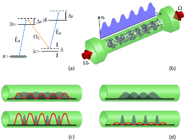
Figure 1: (Color online) In (a) and (b) an ensemble of cold atoms with a 4-level structure is interacting with a pair of classical fields $\Omega_{\pm}$ which create an effective stationary Bragg grating. The photons carried by the input pulse $E^{+}$ coming in from the left are mapped to stationary excitations (polaritons) which are trapped in the grating. The strong photon nonlinearity induced by the 4th level leads to the creation of a strongly interacting gas (grey areas in (c) and (d). By modulating the density of the cold atomic ensemble, an effective lattice potential for polaritons/photons can be created-shown by red lines in (c) and (d). Tuning to the regime of weak interactions between polaritons and adjusting the lattice depth, the system undergoes a BH phase transition from SF (upper one) to MI (lower one) phase (c). In the opposite regime of strong interactions, the dynamics are described by the sG model where the addition of an even shallow polaritonic potential a “pinning transition” for polaritons (d) could be observed. As soon as the desired correlated state is engineered, $\Omega_{-}$ is switched off, and the excitations propagate out of the fiber as correlated photons. The necessary correlations measurements to probe the phases of the system can be performed using standard optical technology on the photons exiting the fiber.

Model setup– The considered atomic level structure is shown in Fig. 1. The one dimensional cold atomic ensemble is prepared outside using standard cold atom techniques and is transferred in the fiber using techniques described in hollow-core . The atoms are initially in the ground state $\left|a\right\rangle$ and the hollow photonic crystal fiber is injected with a quantum coherent pulse $\hat{E}_{+}$ from the left side while a pair of classical fields $\Omega_{\pm}$ are driving the atomic gas from both two sides (Fig. 1(b)). The atomic $\Lambda$ configuration consisting of states $\left|a,b,c\right\rangle$ comprises the typical stationary light set-up reviews ; DPS . Setting the energy of atomic level $a$ to be zero and the atomic levels $b$, $c$, and $d$ to $-\omega_{q}+\Delta_{0}$, $-\omega_{cc}+\delta$, and $-\omega_{cc}-\omega_{q}+\Delta_{p}$, the Hamiltonian describing the four-level atoms, the quantum and classical fields, and their interaction is written as (in the interaction picture)

$$H = -\int n_{a}dz\{\delta\sigma_{cc}+\Delta_{0}\sigma_{bb}+\Delta_{p}\sigma_{dd}$$ (1)

$$+\left(g_{ba}\sigma_{ba}+g_{dc}\sigma_{dc}\right)\left(\hat{E}_{+}e^{ik_{q}z}+\hat{E}_{-}e^{-ik_{q}z}\right)$$

$$+\sigma_{bc}\left(\Omega_{+}e^{ik_{c}z}+\Omega_{-}e^{-ik_{c}z}\right)+h.c.\},$$

where $\sigma_{ij}\equiv\sigma_{ij}\left(z,t\right)=\left|i\right\rangle\left\langle j\right|$, $\hat{E}_{\pm}\equiv\hat{E}_{\pm}\left(z,t\right)=\sum_{k}a_{k}e^{\pm i\left(k-k_{q}\right)z}e^{-i\left(\omega_{k}-\omega_{q}\right)t}$, and $\Omega_{\pm}\equiv\Omega_{\pm}\left(z,t\right)=\sum_{k}fe^{\pm i\left(k-k_{c}\right)z}e^{-i\left(\omega_{k}-\omega_{c}\right)t}$. $\sigma_{ij}$ are collective and continuous operators describing the average of $\left|i\right\rangle\left\langle j\right|$ over atoms with density $n_{a}$ in a small but macroscopic region around $z$, where $i$, $j$ go over $a$, $b$, $c$, and $d$. The fields $\hat{E}_{\pm}$ couple the ground state $\left|a\right\rangle$ to excited state $\left|b\right\rangle$ with a strength given by $g_{ba}$, and $\left|c\right\rangle$ to $\left|d\right\rangle$ with a strength $g_{dc}$. The metastable state $\left|c\right\rangle$ and $\left|b\right\rangle$ are coupled by classical, counter-propagating control fields $\Omega_{\pm}$. The quantum field and classical field envelopes are slowly varying operators and $k_{q}$ and $k_{c}$ are the wavevectors corresponding to their central frequencies $\omega_{q}$ and $\omega_{c}$ for $\hat{E}_{\pm}$ and $\Omega_{\pm}$, respectivelyDPS .

The evolution of $\hat{E}_{\pm}$ in the fiber is described by the Maxwell-Bloch equation as

$$\left(\partial_{t}\pm v\partial_{z}\right)\hat{E}_{\pm}=-iv\Delta\omega\hat{E}_{\pm}+i\sqrt{2\pi}n_{a}\left(g_{ba}\sigma_{ab,\pm}+g_{dc}\sigma_{cd,\pm}\right),$$ (2)

where the slowly varying operators $\sigma_{ab}=\sigma_{ab,+}e^{ik_{q}z}+\sigma_{ab,-}e^{-ik_{q}z}$ and $\sigma_{cd}=\sigma_{cd,+}e^{ik_{q}z}+\sigma_{cd,-}e^{-ik_{q}z}$ are introduced. $v$ is the light speed in the empty waveguide, $v=\omega_{q}/k_{q}$ and $\Delta\omega$ is the difference between $\omega_{q}$ and $\omega_{c}$

We assume that the atoms are initialized in the ground state $\left|a\right\rangle$ and the quantum field is a weak coherent state containing roughly ten photons. Following the standard methods for treating slow light polaritons analyzed in DPS ; Chang-Angelakis , and setting the coupling constants $g_{ba}=g_{dc}=g$ for simplicity, we introduce $\Psi_{+}$, $\Psi_{-}$ as the forward- and backward-going polaritons. These are the propagating excitations and are defined as $\Psi_{\pm}=\cos\theta\hat{E}_{\pm}-\sin\theta\sqrt{2\pi n_{a}}\sigma_{ca}$ with $\cos\theta=\Omega_{\pm}/\sqrt{\Omega_{\pm}^{2}+2\pi g^{2}n_{a}}$ and $\sin\theta=g\sqrt{2\pi n_{a}}/\sqrt{\Omega_{\pm}^{2}+2\pi g^{2}n_{a}}$. In the limit $g\sqrt{2\pi n_{a}}\gg\Omega_{\pm}$, i.e. $\sin\theta\simeq 1$, the excitations are mostly in the spin-wave form, $\Psi_{\pm}=g\sqrt{2\pi n_{a}}\hat{E}_{\pm}/\Omega_{\pm}$, with a group velocity given by $v_{g}\simeq v\Omega^{2}/\left(\pi g^{2}n_{a}\right)$. Next we adiabatically eliminate the fast rotating term from Eq. (2) and set $\Psi=\left(\Psi_{+}+\Psi_{-}\right)/2$ as the stationary combinations. In the limit of a large optical depth , the equations of motion for $\Psi$ read

$$i\partial_{t}\Psi=-\frac{1}{2m}\partial_{z}^{2}\Psi+V\Psi+2\chi\Psi^{\dagger}\Psi^{2}.$$ (3)

The effective mass is $m=-\Delta\omega/(2vv_{g})-\Gamma_{\mathrm{1D}}n_{a}/(4\Delta_{0}v_{g})$, the potential strength is $V=\Delta\omega v_{g}/v-\Lambda\Gamma_{\mathrm{1D}}\delta v_{g}n_{a}/(4\Omega^{2})$ and the interaction strength between polaritons is $\chi=\Lambda^{2}\Xi\Gamma_{\mathrm{1D}}v_{g}/(2\Delta_{p})$ where $\Lambda=\Omega^{2}/(\Omega^{2}-\delta\Delta_{0}/2)$ and $\Xi=(\Delta_{p}-\delta/2)/(\Delta_{p}-\delta)$.

Adding a periodic potential– The nonlinear Schrödinger equation (3) determines the evolution of the trapped polaritonic field $\Psi\left(z,t\right)$ as derived from the effective Hamiltonian, $H=\int dz\Psi^{\dagger}\left(-\frac{\hbar^{2}}{2m}\nabla^{2}+V\right)\Psi+\chi\int dz\Psi^{\dagger}\Psi^{\dagger}\Psi\Psi.$ To add an effective polaritonic lattice, we induce a periodic atomic density distribution by applying an external field such that the atoms in $\left|a\right\rangle$ are now given by $n_{a}=n_{0}+n_{1}\cos^{2}(\pi n_{\mathrm{ph}}z)$. We keep $n_{0}\gg n_{1}$ which means the modulation is only a perturbation in the atomic density and derive the new Hamiltonian which reads

$$H = \int dz\Psi^{\dagger}\left[-\frac{\hbar^{2}}{2m}\nabla^{2}+V_{0}+V_{1}\cos^{2}(\pi n_{\mathrm{ph}}z)\right]\Psi$$ (4)

$$+\chi\int dz\Psi^{\dagger}\Psi^{\dagger}\Psi\Psi,$$

where $V_{0}=\Delta\omega v_{g}/v-\Lambda\Gamma_{\mathrm{1D}}\delta v_{g}n_{0}/(4\Omega^{2})$ is the corresponding trapping polaritonic potential and $V_{1}=-\Lambda\Gamma_{\mathrm{1D}}\delta v_{g}n_{1}/(4\Omega^{2})$ the resulting imposed polaritonic lattice depth. We stress here the dependance of the effective polaritonic lattice on both the slow light parameters (group velocity, trapping laser detuning and strength), and the modulated atomic density. Finally, we note that the atomic lattice modulation should be chosen to be commensurate to the number of the photons in the initial pulse for the pinning transition to occurHaller . This mean the modulation length will approximately fall in the microwave regime as the numbers of trapped photons in the initial pulse is of the order of 10 and the fiber is a few cm in length.

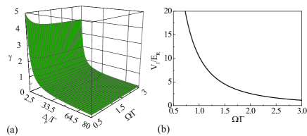
Figure 2: (Color online) Plots of the Lieb-Liniger interaction parameter $\gamma$ as a function of the one-photon detuning $\Delta_{p}/\Gamma$ and the Rabi frequency $\Omega/\Gamma$ of the classical laser field (a) and the lattice depth $V_{1}/E_{\mathrm{R}}$ as a function of $\Omega/\Gamma$ (b). The parameters are taken as $n_{a}=10^{7}\mathrm{m}^{-1}$, $n_{1}=0.1n_{a}$, $n_{\mathrm{ph}}=10^{3}\mathrm{m}^{-1}$, and $\Gamma_{\mathrm{1D}}=0.2\Gamma$, $\Delta_{0}=5\Gamma$, $\delta=0.01\Gamma$ with $\Gamma\simeq 20\mathrm{MHz}$ the atomic decay rate.

Reaching the relevant correlated regimes– The success of achieving a specific strongly correlated polaritonic/photonic state will be characterized by the feasibility of tuning the Lieb-Liniger ratio of the interaction and kinetic energies $\gamma$, and the ratio of the depth of the polaritonic potential to the recoil energy $V_{1}/E_{R}$ to the relevant regimesbooks ; Jaksch . In our system these two quantities read:

$$\gamma = \frac{m\chi}{n_{\mathrm{ph}}}=-\frac{\Lambda^{2}\Xi}{8}\frac{\Gamma_{\mathrm{1D}}^{2}}{\Delta_{0}\Delta_{p}}\frac{n_{0}}{n_{\mathrm{ph}}},$$ (5)

$$\frac{V_{1}}{E_{\mathrm{R}}} = \frac{\Lambda}{8\pi^{2}}\frac{\Gamma_{\mathrm{1D}}^{2}}{\Omega^{2}}\frac{\delta}{\Delta_{0}}\frac{n_{0}n_{1}}{n_{\mathrm{ph}}^{2}}.$$ (6)

Assuming fixed atomic and photonic densities, both quantities can be controlled by tuning the one-photon detuning $\Delta_{p}/\Gamma$ (shifting the fourth level $|d\rangle$ to/from to resonance) and by changing the strength of the control Rabi frequency $\Omega$. In Fig. 2 we plot the achievable regimes for $\gamma$ and $V_{1}/E_{\mathrm{R}}$ as a function of the $\Delta_{p}/\Gamma$ and $\Omega/\Gamma$ of the classical control laser field for realistic parameters. We assume a total atomic decay rate from the upper level $\Gamma\simeq 20\mathrm{MHz}$, approximately atomic density is $n_{0}=10^{7}\mathrm{m}^{-1}$ ($10^{5}$ atoms into a $1\mathrm{cm}$ length fiber) and a photonic density of $n_{\mathrm{ph}}=10^{3}\mathrm{m}^{-1}$ (the input quantum light pulse containing roughly $10$ photons). For these values, $\gamma$ and $V_{1}/E_{\mathrm{R}}$ can be tuned in the range $0$ to $5$ and from $0$ to $20$ respectively, which allows for both the strong and weak interaction regimes to be realized with our trapped polaritonic gas. We note that the current state of the art in the number of atoms loaded in similar hollow-core fibres is smaller by roughly one order of magnitude or less. However, recent experimental progress in the field show that our requirements should be satisfied in the very near futurehollow-core . The losses which will mainly occur due to spontaneous emission from the upper levels, can be estimated by including the corresponding terms in the Hamiltonian Eq. (4). In that case, the effective parameters will acquire an imaginary part which for the effective mass for example will read $m=-\Delta\omega/(2vv_{g})-\Gamma_{\mathrm{1D}}n_{a}/(4\Delta_{0}v_{g}+2i\Gamma v_{g})$, leading to a loss rate $\kappa=\frac{n_{\mathrm{ph}}^{2}v_{g}\Gamma}{n_{a}\Gamma_{\mathrm{1D}}}$. These losses will set an upper bound on the timescales for the preparation of the states, and the probing of the established correlations. For the values under consideration in Fig. 2 and typical slow light velocities $v_{g}$ of 100m/sDPS , these translate to lifetimes of hundreds of micro-seconds. The latter are within the reach of current optical measurement technology.

Polaritonic/photonic pinning transition– We will now discuss the nature of the many body states generated by the addition of the effective polaritonic potential and show that a “pinning transition” for polaritons can be observed, similar to the one recently experimentally verified for bosonic atoms in Haller . This polaritonic pinning transition is expected to transform continuously into the BH regime for a sufficiently deep effective lattices (large $V_{1}/E_{\mathrm{R}}$) and small interactions $\gamma$. To analyze each relevant phase of the system, we will make use of the corresponding BH and sG models from many body physicsbooks . We will also discuss the feasibility to access the whole of the relevant phase diagram for both cases, by simply tuning the optical parameters in our system.

We first analyze the strong interaction regime $1\leq\gamma\leq 5$, and for a weak effective potential, $V_{1}/E_{\mathrm{R}}\leq 3$. This regime is clearly accessible in our photonic system as we show in Fig. 2, by appropriate tuning of the one photon detuning $\Delta_{p}$ and the control laser strength $\Omega$. In this case the proper low-energy description of the system described in Eq. (4), is given by the quantum sG model which readsbooks

$$H=\int\frac{dz}{2}\left\{\frac{\hbar v_{g}}{\pi}\left[\left(\partial_{z}\theta\right)^{2}+\left(\partial_{z}\phi\right)^{2}\right]+V_{1}n_{\mathrm{ph}}\cos\left(4K\theta\right)\right\}.$$ (7)

The first two terms account for the kinetic and interaction energies of polaritons respectively and $\partial_{z}\theta$ and $\partial_{z}\phi$ denote the fluctuations of the long-wavelength density and phase fields $\theta$ and $\phi$ books . The dimensionless parameter $K=\hbar n_{\mathrm{ph}}\pi/\left(mv_{g}\right)$ is known to be related to $\gamma$ as $K\simeq\pi/\sqrt{\gamma-\gamma^{3/2}/\left(2\pi\right)}$ for $\gamma\leq 10$.

On the other hand, if we tune the system to the weak interaction limit with small $\gamma\leq 1$ and large $V_{1}/E_{\mathrm{R}}$ with $V_{1}/E_{\mathrm{R}}\gg 1$, the system is characterized in a good approximation by the BH modelJaksch ,

$$H=-J\sum_{i}\left(b_{i}^{\dagger}b_{i+1}+H.c.\right)+\frac{U}{2}\sum_{i}n_{i}\left(n_{i}-1\right),$$ (8)

where $J/E_{\mathrm{R}}=4\left(V_{1}/E_{\mathrm{R}}\right)^{3/4}\exp\left(-2\sqrt{V_{1}/E_{\mathrm{R}}}\right)/\sqrt{\pi}$, $U/E_{\mathrm{R}}=\sqrt{2/\pi^{3}}\left(V_{1}/E_{\mathrm{R}}\right)^{1/4}\gamma$.

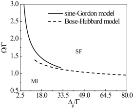
Figure 3: The phase diagram for sG model (large $\gamma$ and small $V_{1}/E_{\mathrm{R}}$) and BH model (small $\gamma$ and large $V_{1}/E_{\mathrm{R}}$). Here $x$- and $y$-axis give the range of tuning parameters $\Delta_{p}$ and $\Omega$ needed for two regimes. The upper region corresponds to SF phase, while the lower region corresponds to MI phase.The rest of the parameters are as in Fig. 2.

In Fig. 3, we show that by simply varying $\Delta_{p}/\Gamma$ and $\Omega/\Gamma$ the whole phase diagram corresponding both to the sG and BH regimes can be accessed in our system for realistic values of the optical parameters. We plot the known phase transition lines corresponding to the sG and BH model occurring at $V_{1}/E_{\mathrm{R}}=2\pi/\sqrt{\gamma-\gamma^{3/2}/\left(2\pi\right)}-4$, and $\left(U/J\right)_{c}=\sqrt{2}\exp\left(2\sqrt{V_{1}/E_{\mathrm{R}}}\right)\gamma/\left[4\pi(V_{1}/E_{\mathrm{R}})^{1/2}\right]\simeq 3.85$ respectivelybooks ; Bloch ; Jaksch . In our case, these are probed by adjusting the detuning and the laser coupling accordingly. The pinning transition is expected to occur for any value $\Delta_{p}/\Gamma$ less than 20 when $\Omega$ is increased to be larger than $\Gamma$ which correspond to vanishing lattice and strong interaction regime $\gamma\geq 3.5$. The BH Mott transition will occur in the opposite weakly interacting regime and deeper lattices. In Fig. 4, for a specific value of the $\Delta_{p}/\Gamma=50$ corresponding to with $\gamma\l 1$, we plot he interaction $U$ and and tunneling strengths as a function of $\Omega/\Gamma$ to further illustrate this case. We see that transition occurs for $\Omega/\Gamma\simeq 1.03388$ which corresponds to known critical point of $\left(U/J\right)_{c}\simeq 3.85$.

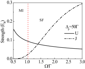
Figure 4: The interaction and tunneling strength as functions of $\Omega/\Gamma$ with $\Delta_{p}=50\Gamma$ for the weakly interacting gas in the BH regime. The red dot line at $\Omega/\Gamma\simeq 1.03388$ corresponds to the Mott phase transition point $\left(U/J\right)_{c}\simeq 3.85$. The rest of the parameters are as in Fig. 2.

We will now summarize the whole process consisting of preparation, evolution and detection of the states. First, the atoms are prepared in state $\left|a\right\rangle$ with a slightly modulated atomic density and transferred in the fiber . Next, $\hat{E}_{+}$ is sent in from the left with a co-propagating control field $\Omega_{+}$ turned on. Once $\hat{E}_{+}$ completely enters the medium, $\Omega_{+}$ is slowly turned off, reversibly converting $\hat{E}_{+}$ into the pure atomic excitations in the usual slow light mannerDPS and the medium is illuminated simultaneously by $\Omega_{+}$ and $\Omega_{-}$, making $\hat{E}_{+}$ quasi-stationary and trapped. The quantities $\gamma$ and $V_{1}/E_{\mathrm{R}}$ are then changed in time to reach the desired state. Finally one of the control fields $\Omega_{-}$ is switched off, mapping the polaritons to photons and releasing the excitations. At this time, the spatial correlations are mapped into temporal correlations of outgoing photons, on which measurements are done using standard quantum optical techniques. By analyzing the resulting photonic spectra and correlation functions the state of system could be obtained.

In conclusion we have shown that different strongly correlated states of photons could be created inside hollow-core fibers interacting with atomic gases with current or near future optical technology. The resulting states can be controllably tuned to reproduce sG and BH many body dynamics and also used to probe the corresponding pinning quantum phase transition predicted by these models. The various correlated phases can be analyzed by standard optical correlations measurements on the light exiting the fiber.

We would like to acknowledge useful discussion by Profs LC Kwek and KS Huang in the early stages of this work and the financial support by the National Research Foundation & Ministry of Education, Singapore.

References

- (1) S. , Quantum Phase Transitions (Cambridge University Press, Cambridge, England, 1999); T. Giamarchi, Quantum Physics in One Dimension (Oxford University Press, Oxford, 2004).
- (2) M. Greiner, O. Mandel, T. Esslinger, T.W. Hansch and I. Bloch, Nature 415 39-44 (2002).
- (3) D. Jaksch, C. Bruder, J.I. Cirac, C.W. Gardiner, and P. Zoller. Cold Bosonic Atoms in Optical Lattices. Phys. Rev. Lett. 81, 3108 (1998).
- (4) H.P. Büchler, G. Blatter, and W. Zwerger, Phys. Rev. Lett. 90, 130401 (2003).
- (5) E. Haller et al., Nature 466, 597-600 (2010).
- (6) A. Friedenaue et al., Nature Phys. 4, 757 - 761 (2008).
- (7) M. J. Hartmann, F. G. S. L. Brandão, and M. B. Plenio, Nature Phys. 2, 849 (2006); D. G. Angelakis, M. F. Santos, and S. Bose, Phys. Rev. A 76, 031805(R) (2007); A. D. Greentree, et al., Nature Phys. 2, 856 (2006).
- (8) H. Walther, B. T. H. Varcoe, B-G Englert and T. Becker. Rep. Prog. Phys. 69: 1325 (2006); M. Fleischhauer, A. Imamoglu and J.P. Marangos. Rev. Mod. Phys. 77, 633 (2005).
- (9) D. Rossini and R. Fazio, Phys. Rev. Lett., 99 186401 (2007); Y.C. Neil Na et al., Phys. Rev. A, 77 031803(R)(2008); M. Aichhorn et al., Phys. Rev. Lett. 100, 216401 (2008); Dario Gerace et al., Nat. Phys. 5, 281 (2009); I. Carusotto et al. , Phys. Rev. Lett. 103, 033601 (2009); D.G. Angelakis et al. Eur. Phys. Lett. 85, 20007 (2009);
- (10) S. Ghosh, et al., Phys. Rev. Lett. 94 093902 (2005); K.P. Nayak, et al, Opt. Express 15 5431-5438 (2007); T. Takekoshi and R.J. Knize, Phys. Rev. Lett. 98 210404 (2007); Christensen C A., et al., Phys. Rev. A 78 033429 (2008); S. Vorrath, et al., New J. Phys. 12 123015 (2010);
- (11) M. Fleischhauer and M.D. Lukin. Phys. Rev. Lett. 84, 5094 (2000); M. Bajcsy, et al., Nature 426, 638 (2003); M. Bajcsy, et al., Phys. Rev. Lett. 102, 203902 (2009); E. Shahmoon, et al., arXiv:1012.3601v1.
- (12) D. E. Chang, et al., Nat. Phys. 4, 884 (2008); D.G.Angelakis et al, arXiv:1006.1644.
- (13) Sague et al. Phys, Rev. Lett, 99, (2007).