Numerical Experiments for Darcy Flow on a Surface
Using Mixed Exterior Calculus Methods

Abstract

There are very few results on mixed finite element methods on surfaces. A theory for the study of such methods was given recently by Holst and Stern, using a variational crimes framework in the context of finite element exterior calculus. However, we are not aware of any numerical experiments where mixed finite elements derived from discretizations of exterior calculus are used for a surface domain. This short note shows results of our preliminary experiments using mixed methods for Darcy flow (hence scalar Poisson’s equation in mixed form) on surfaces. We demonstrate two numerical methods. One is derived from the primal-dual Discrete Exterior Calculus and the other from lowest order finite element exterior calculus. The programming was done in the language Python, using the PyDEC package which makes the code very short and easy to read. The qualitative convergence studies seem to be promising.

1 Introduction

In this short note we present results from some preliminary numerical experiments for Darcy flow (hence scalar Poisson’s equation in mixed form) on a surface. We use two mixed methods. One is derived from primal-dual Discrete Exterior Calculus (DEC) and adapted from [5]. The other method uses the $\mathcal{P}_{1}^{-}\Lambda^{1}$ elements, i.e., Whitney 1-forms for the fluxes, and piecewise constants for the pressures. We’ll refer to this second method as being derived from finite element exterior calculus (FEEC) [2, 3] or call it the Whitney solution. Switching between the DEC and FEEC methods requires a 1 line change in our code, which is written in Python using PyDEC [4]. The only difference between the two methods in our code is that the former method uses a primal-dual DEC Hodge star, and the latter uses Whitney Hodge star [4]. The surface used is a hemisphere with a hole punched out around north pole, and we will refer to this surface as an annular hemisphere. The boundary conditions are Neumann for pressure, hence specified as flux on the boundary. The pressure is fixed arbitrarily at a point to make the problem well-posed. The use of the Whitney Hodge star is equivalent to a solution using finite element exterior calculus. Recall that the equations of Darcy flow on domain $M$ are:

$$v+\operatorname{grad}p =0 \quad\text{on }M$$

$$\operatorname{div}v =0 \quad\text{on }M$$

$$v\cdot\hat{n} =\psi \quad\text{on }\partial M$$

where we have assumed the ratio of permeability and viscosity to be 1 and assumed the absence of sources and sinks in the domain. The unknowns are the pressure $p$ and velocity $v$, in $M$. In mixed FEM literature, the preferred variable names are $u$ and $\sigma$, respectively.

2 Exterior Calculus Mixed Methods

In exterior calculus notation, taking $p$ to be a 0-form the Darcy flow equations can be written in terms of the 1-form proxy for the vector field, and the exterior derivative of the pressure. The divergence is replaced by the codifferential. In particular, on domain $M$, the Darcy equations from above become

$$v^{\flat}+\operatorname{d}p =0\,,$$

$$-\delta v^{\flat} =0\,,$$

where $\flat$ is the isomorphism between vector fields and 1-forms and $\delta$ is the codifferential [1]. Applying a Hodge star to the first equation and using $\delta=-\operatorname{\ast}\operatorname{d}\operatorname{\ast}v^{\flat}$ we have

$$\operatorname{\ast}v^{\flat}+\operatorname{\ast}\operatorname{d}p =0\,,$$

$$\operatorname{d}\operatorname{\ast}v^{\flat} =0\,.$$

We will set $\sigma=\operatorname{\ast}v^{\flat}$ which is a flux, and use that as an unknown. The above equations for a 2-dimensional domain are equivalent to

$$\operatorname{\ast}\sigma-\operatorname{d}p =0\,,$$

$$\operatorname{d}\sigma =0\,.$$

Following [5] we discretize this as

$$\begin{bmatrix}-\operatorname{\ast}_{1}&\operatorname{d}_{1}^{T}\\ \phantom{-}\operatorname{d}_{1}&0\end{bmatrix}\begin{bmatrix}\sigma\\ p\end{bmatrix}=\begin{bmatrix}0\\ 0\end{bmatrix}\,,$$

where the coboundary matrix $\operatorname{d}_{1}$ is the transpose of the boundary matrix $\operatorname{\partial}_{2}$ from triangles to edges. This linear system is made nonsingular by fixing pressure at a point and adjusting the system for this. For more details on the above derivation see [5]. When $\operatorname{\ast}_{1}$ is the mass matrix for Whitney 1-forms, i.e., Whitney Hodge star, one gets a finite element exterior calculus type Whitney solution. When $\operatorname{\ast}_{1}$ is the primal-dual DEC Hodge star, one gets the DEC method of [5]. Both these methods are used in this paper.

In the code, a simplicial_complex object of PyDEC is created after reading the mesh from files. If sc is the name of this object, then the choice between Whitney or DEC solution requires only specifying the appropriate Hodge star matrix in the Python code. For the Whitney Hodge star, which yields the Whitney solution, one writes

⬇

star1 = whitney_innerproduct(sc, 1)

and for the primal-dual DEC Hodge star, which yields the DEC solution, one writes

⬇

star1 = sc[1].star

The matrix of the system above is assembled by the code

⬇

A = bmat([[(-mu/k)*star1, sc[1].d.T],

[sc[1].d, None]], format=’csr’)

where csr refers to the compressed sparse row format, one of many sparse matrix formats available via SciPy. The variables mu and k refer to the viscosity and permeability and for this note we are assuming this ratio to be 1. The main programming effort in the rest of the code is in the quadratures needed for the exact flux and in setting the boundary conditions.

Thus the numerical methods use flux as a 1-cochain associated with the edges, and pressure associated with the triangles. In DEC the pressure is a dual 0-cochain associated with the circumcenters of the triangles of the mesh which needs to be Delaunay. In the Whitney solution the pressure is considered constant on each triangle. For visualization, we interpolate the flux using a Whitney map and sample it at the barycenters of the triangles and rotate it by $\pi/2$.

3 Planar Annulus as a Preparatory Exercise

To motivate the solution on the annular hemisphere we first discuss the case of planar annulus. Consider a planar annulus with origin as center, inner radius $r_{0}$ and outer radius $r_{1}$. The fluid enters from the inner boundary and exits through the outer boundary. We will take the direction of the flow to be normal to the boundary and speed to be constant along the inner boundary. At the inflow boundary velocity vectors are pointing into the domain, and at the outflow boundary they are pointing out of the domain. By symmetry, the velocity at any point will be directed radially pointing away from the origin. The speed along a circle of radius $r$ will be constant. The magnitude of velocity can be determined by using divergence theorem as follows.

Let $D_{r}$ be an open disk of radius $r\,,r_{0}<r\leq r_{1}$, and let $M_{r}=M\cap D_{r}$ be the annulus with the inner radius $r_{0}$ and outer radius $r$. Since there are no sources and sinks (i.e., $\operatorname{div}v=0\text{ in }M$), we have

$$0=\int\limits_{M_{r}}\operatorname{div}v\,dx=\int\limits_{\partial M_{r}}v\cdot\hat{n}\,d\gamma\,,$$

where $d\gamma$ is the measure on the boundary. If $\Gamma_{0}$ is the inner circle and $\Gamma$ the outer circle, we have

$$\int\limits_{\Gamma_{0}}v(x,y)\cdot\hat{n}(x,y)\,d\gamma=\int\limits_{\Gamma}v(x,y)\cdot\hat{n}(x,y)\,d\gamma\,,$$ (1)

Since $v\cdot\hat{n}$ is a constant on any circle, let us call the first integrand $S(r_{0})$ and the second one $S(r)$. Then we have $S(r_{0})\,2\pi r_{0}=S(r)\,2\pi r$, or

$$S(r)=S(r_{0})\dfrac{r_{0}}{r}\,.$$

The norm of the velocity on outer circle of the original annulus is $S(r_{0})r_{0}/r_{1}$. From the expression for speed we can determine the pressure at any $r$ as follows. Along a ray from origin, we have a one dimensional problem and

$$S(r)=-\dfrac{dp}{dr}\,.$$

Thus $p(r)$ along any ray is given by

$$p(r)=-\int\limits_{r_{0}}^{r}S(\xi)\,d\xi+C_{0}=-S(r_{0})r_{0}\int\limits_{r_{0}}^{r}\dfrac{1}{\xi}\,d\xi+C_{0}\,,$$

where $C_{0}$ is the arbitrary pressure at $r_{0}$. Thus

$$p(r)=-S(r_{0})r_{0}\left.\ln r\right|_{r_{0}}^{r}+C_{0}=-S(r_{0})r_{0}\ln r+C$$

where $C=C_{0}+S(r_{0})r_{0}\ln r_{0}$, hence just another arbitrary constant. In our code we took $C_{0}=0$, and hence $C=S(r_{0})r_{0}\ln r_{0}$. In fact since the experiments use an annulus with $r_{0}=1$ even $C=0$ in these experiments.

Numerical results for planar annulus

We computed the pressure as a 0-cochain and flux as a 1-cochain. In the DEC solution the pressure is a dual 0-cochain associated with the circumcenters even if the circumcenter is outside the triangle, as long as it is Delaunay [4]. In the Whitney solution solution, pressure is assumed constant on each triangle. The results of the annulus experiments are shown for the Whitney solution in Figures 1 and 2 and for DEC in Figure 3. Figure 1 shows the velocity vector field sampled at the barycenter of each triangle. Figures 2 and 3 show the speed and pressure as a function of $r$ for the two different methods. In both, the Whitney solution plots and the DEC plots, for the purpose of visualization, the location for the pressure in a triangle was associated with its circumcenter. That is the value of $r$ used for a particular computed pressure was that of the circumcenter of the triangle. The flux was interpolated using a Whitney map and sampled at the barycenter and thus the $r$ value of the barycenter was used for drawing the speed plots. Qualitative studies of convergence are in Figure 4 and 5. We started with a coarse mesh of 484 triangles and refined it by subdividing each triangle into 4 congruent triangles to obtain meshes with 1,516 and 14,685 triangles.

4 Annular Hemisphere

Now we will consider a hemispherical domain with a circular hole punched out around north pole. The bottom boundary sits on the $xy$-plane and the $z$-axis points up. Two of the triangulations of the domain that we use are shown in Figure 6. The inflow is now from the top boundary and the outflow at the equator. Both are tangential to the surface and normal to the boundary.

The derivation of the analytical solution closely follows the derivation for the planar annulus. By symmetry the speed at a fixed latitude will be constant, with velocity normal to the latitude and tangential to the sphere. The divergence theorem can be used as in the planar case and the shape of the surface between the two latitudes is irrelevant. Consider any point on the surface where the velocity and pressure are desired. Let $r$ be the horizontal distance of this point from the $z$-axis. The derivation for speed follows the one of planar annulus, with $\Gamma_{0}$ being the top boundary and $\Gamma_{r}$ being the latitude passing through the point that is distance $r$ from the $z$-axis.

For deriving the pressure solution, we will use spherical coordinates with the convention that $\theta$ is measured from $z$-axis and $\phi$ is measured from the $x$-axis. Since the radius of the hemisphere is 1, we will use $r$ to stand for the distance from $z$-axis. By symmetry, the only nonzero component for $v$ is in the $\theta$-direction. We will call this component $S(\theta)$. By the planar annulus derivation,

$$S(\theta)=S(\theta_{0})\,\dfrac{\sin\theta_{0}}{\sin\theta}\,,$$

where $\theta_{0}$ corresponds to the latitude at $r_{0}$ distance from the $z$-axis. Thus,

$$\frac{dp}{d\theta}=-S(\theta_{0})\,\dfrac{\sin\theta_{0}}{\sin\theta}\,,$$

which implies

$$p(\theta)=-S(\theta_{0})\,\sin\theta_{0}\int\limits_{\theta_{0}}^{\theta}\dfrac{1}{\sin\xi}d\xi+C_{0}\,,$$

for an arbitrary constant $C_{0}$. Thus,

$$p(\theta)=S(\theta_{0})\,\sin\theta_{0}\;\ln\left(\dfrac{1+\cos\theta}{\sin\theta}\right)+C\,,$$

and we use

$$C=-S(\theta_{0})\,\sin\theta_{0}\;\ln\left(\dfrac{1+\cos\theta_{0}}{\sin\theta_{0}}\right)+C_{0}\,,$$

with $C_{0}$ set to 0 in our code.

Numerical results for annular hemisphere

The results for the annular hemisphere experiments are shown in Figures 7-11. For every mesh used in these experiments the vertices always lie on the hemisphere surface. For the DEC based method we use a well-centered mesh, that is one in which each triangle is acute [6] although a weaker condition can be imposed on the mesh. For the Whitney solution method no such conditions are required. For completeness we used well-centered as well as non well-centered meshes when computing Whitney solutions. Some representative speed and pressure plots for the Whitney solution are in Figure 7 and for DEC in Figure 8. For the purpose of visualizing the computed pressures an $r$ value has to be associated with the computed pressure corresponding to a triangle. For a well-centered mesh we use the $r$ value of the circumcenter projected to the hemisphere and for other meshes we use the projected barycenters. The flux is interpolated and sampled at barycenter as described in the planar case. For this flux, the $r$ value used is that of the barycenter projected to the hemisphere.

5 Conclusions and Future Work

Our experience has been that it is easy to conduct numerical experiments for Darcy flow on a surface with DEC and lowest order FEEC using the Python package PyDEC [4]. It would be interesting to compare this with the programming effort required for a vector calculus formulation on surfaces using classical mixed finite elements. To continue the exterior calculus based experimentation, we plan to do numerical experiments on the surface used here using different boundary conditions, do computations using other surfaces, and do quantitative convergence studies besides the qualitative studies shown here.

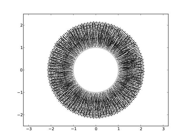
Figure 1: The velocity field corresponding to the flux on a planar annulus computed as a Whitney solution. The boundary condition is Neumann and pressure is fixed arbitrarily at a single point. The inflow is constant speed entry at inner boundary and constant speed exit at outer boundary whose value can be computed using the divergence theorem. The profiles for speed and pressure are in Figure 2. The planar annulus here is used as a warmup exercise for the surface experiments on an annular hemisphere.

Figure 2: Numerical solution for planar annulus computed as a Whitney solution, compared with analytical solution. Left plot shows a scatter plot of the speeds compared with the analytical values over a ray from the inner to outer boundary of the annulus. Right plot is a similar plot for the pressures.

Figure 3: Numerical results for planar annulus computed using DEC. The two plots are similar to the ones in Figure 2.

Figure 4: A qualitative indication of convergence of the Whitney solution for the planar annulus on a series of Delaunay meshes similar to the one shown in Figure 1. Similar to Figure 2, the left panels are speed plots and the right ones are pressure plots. The rows of figures from top to bottom are profiles on increasingly finer meshes with 484, 1516 and 14685 elements, respectively.

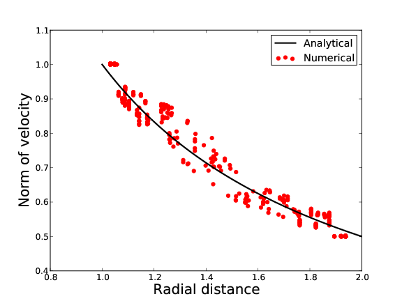
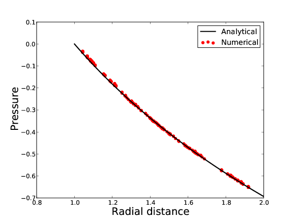
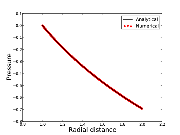
Figure 5: A qualitative indication of convergence of DEC solution for the planar annulus on a series of Delaunay meshes similar to the one shown in Figure 1. Similar to Figure 2, the left panels are speed plots and the right ones are pressure plots. The rows of figures from top to bottom are profiles on increasingly finer meshes with 484, 1516 and 14685 elements, respectively.

Figure 6: Representative triangulations of the annular hemisphere. The top mesh is generated from the mesh generation software gmsh, and the bottom mesh is a well-centered triangulation [6] obtained using Python code. The mesh in the top figure consists of 4928 triangles. The speed and pressure profiles for Whitney solution obtained using a similar mesh consisting of 138536 triangles is shown in Figure 7. The bottom mesh consists of 6600 triangles. The speed and pressure profiles for DEC solution obtained using a similar mesh consisting of 135900 triangles is shown in Figure 8.

Figure 7: Whitney solution for an annular hemisphere of the type shown in top of Figure 6. Left figure here shows a scatter plot of the speeds compared with the analytical values over a longitude from the top to bottom boundary. Right figure shows a similar plot for the pressures.

Figure 8: DEC solution for a well-centered triangulation of a punctured hemisphere of the type shown in bottom of Figure 6. The two plots are similar to the ones in Figure 7.

Figure 9: A qualitative indication of convergence of the Whitney solution for the annular hemisphere on a series of non well-centered meshes similar to the mesh shown in the top panel of Figure 6. Similar to Figure 7, the left panels are speed plots and the right ones are pressure plots. The rows of figures from top to bottom are profiles on increasingly finer meshes with 240, 1096 and 4928 elements, respectively.

Figure 10: A qualitative indication of convergence of DEC solution for the annular hemisphere on series of well-centered meshes similar to the one in the bottom panel of Figure 6. Similar to Figure 7, the left panels are speed plots and the right ones are pressure plots. The rows of figures from top to bottom are profiles on increasingly finer meshes with 240, 6600 and 15000 elements, respectively.

Figure 11: A qualitative indication of convergence of the Whitney solution for the annular hemisphere on series of well-centered meshes similar to the one in the bottom panel of Figure 6. Similar to Figure 7, the left panels are speed plots and the right ones are pressure plots. The rows of figures from top to bottom are profiles on increasingly finer meshes with 240, 6600 and 15000 elements, respectively.

References

- [1] Abraham, R., Marsden, J. E., and Ratiu, T. Manifolds, Tensor Analysis, and Applications, second ed. Springer–Verlag, New York, 1988.
- [2] Arnold, D. N., Falk, R. S., and Winther, R. Finite element exterior calculus, homological techniques, and applications. In Acta Numerica, A. Iserles, Ed., vol. 15. Cambridge University Press, 2006, pp. 1–155.
- [3] Arnold, D. N., Falk, R. S., and Winther, R. Finite element exterior calculus: from Hodge theory to numerical stability. Bull. Amer. Math. Soc. (N.S.) 47, 2 (2010), 281–354. doi:10.1090/S0273-0979-10-01278-4.
- [4] Bell, N., and Hirani, A. N. PyDEC: Algorithms and software for Discretization of Exterior Calculus, March 2011. Available as e-print on arxiv.org. arXiv:1103.3076v1.
- [5] Hirani, A. N., Nakshatrala, K. B., and Chaudhry, J. H. Numerical method for Darcy flow derived using Discrete Exterior Calculus. Tech. Rep. UIUCDCS-R-2008-2937, Department of Computer Science, University of Illinois at Urbana-Champaign, 2008. Also available as e-print on arxiv.org. arXiv:0810.3434v3.
- [6] VanderZee, E., Hirani, A. N., Guoy, D., and Ramos, E. A. Well-centered triangulation. SIAM Journal on Scientific Computing 31, 6 (2010), 4497–4523. Also available as e-print on arxiv.org. arXiv:0802.2108v3, doi:10.1137/090748214.