Shock formation in stellar perturbations and tidal shock waves in binaries

Abstract

We investigate whether tidal forcing can result in sound waves steepening into shocks at the surface of a star. To model the sound waves and shocks, we consider adiabatic non-spherical perturbations of a Newtonian perfect fluid star. Because tidal forcing of sounds waves is naturally treated with linear theory, but the formation of shocks is necessarily nonlinear, we consider the perturbations in two regimes. In most of the interior, where tidal forcing dominates, we treat the perturbations as linear, while in a thin layer near the surface we treat them in full nonlinearity but in the approximation of plane symmetry, fixed gravitational field and a barotropic equation of state. Using a hodograph transformation, this nonlinear regime is also described by a linear equation. We show that the two regimes can be matched to give rise to a single mode equation which is linear but models nonlinearity in the outer layers. This can then be used to obtain an estimate for the critical mode amplitude at which a shock forms near the surface. As an application, we consider the tidal waves raised by the companion in an irrotational binary system in circular orbit. We find that shocks form at the same orbital separation where Roche lobe overflow occurs, and so shock formation is unlikely to occur.

1 Introduction

As far as we are aware it is unknown if the tidal forces in a binary inspiral can create shock waves before the binary objects touch, begin mass transfer or plunge. In order to investigate this, we have developed a quantitative criterion for the critical amplitude at which stellar perturbations form shocks that may be interesting in its own right, or in other applications.

This work was originally motivated by the observation of unsmooth fluid behaviour in the numerical simulation of an irrotational, equal mass neutron star (NS) binary merger (Baiotti et al. (2008); Rezzolla et al. (2010)). The simulations show surface waves breaking when the initial data are evolved with the cold equation of state (EOS) $P=K\rho^{2}$ , and a strong wind when they are evolved with the equivalent hot EOS $P=\rho e$ (with initially constant entropy). As both simulations should be identical until genuine shocks form, it seems likely that both the wind and the surface waves are artefacts of the interaction with the artificial atmosphere. On the other hand, these artefacts may also hide genuine shocks.

Mass shedding in small amplitude nonlinear perturbations has been demonstrated numerically for neutron stars rotating near the mass-shedding angular velocity (Stergioulas et al. (2006); Dimmelmeyer et al. (2004)), but the minimum perturbation amplitude for this to occur has not been quantified.

We have therefore tried to obtain a quantitative criterion for shock formation using a combination of stellar perturbation theory and nonlinear planar fluid dynamics. We consider a shock formation scenario where essentially radial sound waves steepen as they approach the surface because the density and sound speed approach zero at the surface. (Note that while the shape of the tidal bulges rotates around the star, individual fluid elements mainly move up and down.)

If such waves are generated by tidal forces from the companion, their amplitude and shape is determined in the bulk of the star, where almost all the mass is. In this regime, linear perturbation theory can be used to obtain the response of the star to the tidal force, treating its proper oscillation modes as forced harmonic oscillators. For simplicity, we assume that the background star is irrotational and spherical.

On the other hand, near the surface the fluid geometry can be approximated as plane-parallel, and entropy or composition gradients become irrelevant compared to the density gradient. In this regime we use a hodograph transform to cast the nonlinear dynamics into a single linear second-order PDE. A shock forms if and only if the hodograph transform becomes singular: a criterion for this can be examined within the model itself (Gundlach & Please (2009)). This criterion was tested in the numerical evolution of nonlinear spherical perturbations of an $n=1$ polytropic star and found to be accurate within 10% (Gabler et al. (2009)). Once formed, these shocks quickly take a universal, self-similar form (Gundlach & LeVeque (2011)).

The two regimes are linked by noting that under certain approximations the fluid variables and their equations of motion in the two regimes coincide near the surface.

In Sec. 2, we derive the combination of linear non-spherical and planar non-linear fluid motion. We summarise the (well-known) linear perturbation equations for adiabatic non-spherical stellar oscillations in a suitable notation, and their limit near the surface if the density vanishes there. We present the hodograph transform and the shock formation criterion. We cast the hodograph equation in a form where it can be identified with the linear perturbation equations near the surface in a high-frequency Cowling approximation. We then evaluate the shock formation criterion on solutions of the linear perturbation equations as if they were solutions of the hodograph equation.

In Sec. 3, we apply this general formalism to waves raised in a star by the tidal force of its binary companion. We can then use standard methods to calculate the reaction to this force by expanding the perturbations in proper oscillation modes. We obtain the orbital separation $d_{\rm crit}$ at which shocks first form as function of the modes of the star and the mass ratio $q$.

In Sec. 4, we carry out the necessary numerical mode calculations for stars with polytropic equations of state. Sec. 5 reviews our main approximations and states our astrophyical conclusions.

A similar calculation to our Sec. 3 has been carried out for $g$-modes in NSs by Lai (1994). Their frequency is lower than the orbital frequency at merger, and so the orbital frequency moves through resonance as the orbit shrinks, and the full time-dependent driven oscillator problem must be considered. It was assumed that no shock forms, and dissipative heating was estimated instead. It turns out that the duration of the resonance is too short to give rise to significant heating. By contrast, we focus on $p$-modes, which have higher frequencies and are never in resonance, and estimate their amplitude adiabatically in the approximation of a stationary circular orbit.

2 Nonlinear extension of linear perturbation modes

2.1 Linear adiabatic perturbation equations

We consider linear adiabatic perturbations of a spherically symmetric static perfect fluid star in Newtonian physics, in the frequency domain. The background is assumed to be non-rotating and in hydrostatic equilibrium. $d/dr$ is denoted by a prime. The background quantities are the density $\rho(r)$, pressure $P(r)$, gravitational potential $\phi(r)$, gravitational acceleration $\phi^{\prime}(r)\geq 0$, sound speed $c(r)$ defined by $c^{2}\equiv(\partial P/\partial\rho)_{s}$, entropy per rest mass $s(r)$, and Brunt-Väisälä frequency $N(r)$ defined by

$$-{N^{2}\over{\phi^{\prime}}}\equiv{\rho^{\prime}\over\rho}-{P^{\prime}\over c^{2}\rho}.$$ (1)

The equations of hydrostatic equilibrium for the spherical background star are

$$P^{\prime}+{\phi^{\prime}}\rho=0,$$ (2)

$$\phi^{\prime\prime}+{2\over r}\phi^{\prime}=4\pi G\rho.$$ (3)

The displacement vector of the (polar) nonspherical perturbation is expanded in spherical harmonics as

$${\vec{\xi}}({\vec{r}},t)\equiv e^{-i\omega t}\ \left[\xi_{r}(r)Y_{lm}(\theta,\varphi){\vec{e}}_{r}+\xi_{h}(r)r{\vec{\nabla}}_{\perp}Y_{lm}(\theta,\varphi)\right],$$ (4)

where

$${\vec{\nabla}}_{\perp}={1\over r}{\vec{e}_{\theta}}{\partial\over\partial\theta}+{1\over r\sin\theta}{\vec{e}_{\varphi}}{\partial\over\partial\varphi}.$$ (5)

Because the equations are linear, it is customary to make $\vec{\xi}$ complex as above for ease of calcuation. The physical displacement is its real part

$$\vec{\xi}_{\rm real}={\rm Re}\,\vec{\xi}.$$ (6)

We neglect axial displacements, which in a non-rotating star have no restoring force, and are zero modes. The (real) fluid velocity is simply the time derivative of the displacement, or

$${\vec{v}}_{\rm real}({\vec{r}},t)={\rm Re}[-i\omega{\vec{\xi}}({\vec{r}},t)].$$ (7)

The Lagrangian perturbation $\delta f$ of any background quantity $f(r)$ is related to the Eulerian perturbation $f_{1}$ by

$$\delta f\equiv f_{1}+{\vec{\xi}}\cdot{\vec{\nabla}}f=f_{1}+\xi_{r}f^{\prime}.$$ (8)

All scalar perturbations are also expanded in spherical harmonics, for example the Eulerian density perturbation

$$\rho_{1}({\vec{r}},t)=e^{i\omega t}\rho_{1}(r)Y_{lm}(\theta,\varphi).$$ (9)

The assumption of adiabatic perturbations is that

$$\delta P=c^{2}\delta\rho.$$ (10)

For given spherical harmonic index $l$, we define the shorthand

$$F(r)\equiv 1-{l(l+1)c^{2}\over\omega^{2}r^{2}}.$$ (11)

The radial and (polar) horizontal parts of the Euler equation and the mass conservation equation can be combined to give a single second-order ODE for $\xi_{r}$. With a later approximation in mind, we write this as

$$\xi_{r}^{\prime\prime}+A\xi_{r}^{\prime}+B\xi_{r}=S,$$ (12)

where

$$A = 2{c^{\prime}\over c}-{F^{\prime}\over F}-{N^{2}\over g}+{2\over r}-{{\phi^{\prime}}\over c^{2}},$$ (13)

$$B = \left(2{c^{\prime}\over c}-{F^{\prime}\over F}-{N^{2}\over{\phi^{\prime}}}\right)\left({2\over r}-{{\phi^{\prime}}\over c^{2}}\right)$$ (14)

$$-{2\over r^{2}}-\left({{\phi^{\prime}}\over c^{2}}\right)^{\prime}+{F\over c^{2}}(\omega^{2}-N^{2}),$$

$$S = {\phi_{1}^{\prime}\over c^{2}}-{l(l+1)\over\omega^{2}r^{2}}\left({N^{2}\over{\phi^{\prime}}}-2{c^{\prime}\over c}+{F^{\prime}\over F}+{2\over r}\right)\phi_{1}.$$ (15)

This is complemented by the perturbed Poisson equation

$$\phi_{1}^{\prime\prime}+{2\over r}\phi_{1}^{\prime}-{l(l+1)\over r^{2}}\phi_{1}=4\pi G\rho_{1}.$$ (16)

Its source term is the Eulerian density perturbation

$$\rho_{1}=-{\rho\over F}\left[\xi_{r}^{\prime}+\left({2\over r}-{{\phi^{\prime}}\over c^{2}}-F{N^{2}\over{\phi^{\prime}}}\right)\xi_{r}-{l(l+1)\over\omega^{2}r^{2}}\phi_{1}\right].$$ (17)

Finally, the complete perturbation can be reconstructed using

$$\xi_{h}(r)={1\over F\omega^{2}r}\left\{-c^{2}\left[\xi_{r}^{\prime}+\left({2\over r}-{{\phi^{\prime}}\over c^{2}}\right)\xi_{r}\right]+\phi_{1}\right\}.$$ (18)

Our second-order equations for $\xi_{r}$ and $\phi_{1}$ can be derived from the first-order systems given in, for example, Unno et al. (1989) and Christensen-Dalsgaard & Mullan (1994).

2.2 Expansion near the surface and boundary conditions

The boundary conditions for $\phi_{1}$ are $\phi_{1}\sim r^{l}$ at $r=0$ and $\phi_{1}^{\prime}+(l+1)\phi_{1}/r=0$ at $r=R$. The boundary condition for $\xi_{r}$ at $r=0$ is $\xi_{r}\sim r^{l-1}$ (Unno et al. (1989)). To find the boundary condition for $\xi_{r}$ at $r=R$, we need to expand the equations to leading order in $x\equiv r-R\leq 0$. In the following, $O(x)$ will be shorthand for $O(|x|/R)$.

We assume that near the surface the EOS is approximated by the Gamma-law EOS

$$P(\rho,e)={\rho e\over n},$$ (19)

where $P$ is the pressure, $\rho$ is the mass density, $e$ the internal energy per rest mass, and $n$ a constant. From the first law of thermodynamics, this is equivalent to

$$P(\rho,s)=K(s)\rho^{1+{1\over n}},$$ (20)

where $s$ is the entropy per rest mass. The form of $K(s)$ does not matter for our purposes (additional input is required to fix it), and more generally $K$ can be considered a function of both entropy and composition to take into account stratification effects in NSs.

For a stratified background star where $K(s)$ is a given function $K(r)$, we find

$$-{N^{2}\over{\phi^{\prime}}}=-{n\over n+1}{K^{\prime}\over K}.$$ (21)

In the literature (for example Shapiro & Teukolsky (2004)), a power-law stratification is often considered which is parameterised by specifying the equilibrium pressure as

$$P(r)=K_{0}\rho(r)^{1+{1\over n_{0}}}\quad\Leftrightarrow\quad K(r)=K_{0}\rho^{{1\over n_{0}}-{1\over n}},$$ (22)

with $n_{0}>n$ required for stability. (Note that $n$ characterises the EOS, $n/n_{0}$ characterises the stratification, and $n_{0}$ appears in the Lane-Emden equation). With $\rho\sim x^{n_{0}}$ as $x\to 0$, we have

$$K(r)\sim x^{1-{n_{0}\over n}},$$ (23)

and so $K$, $K^{\prime}$ and $N$ all diverge as $x\to 0$. Clearly this assumption is unphysical on sufficiently small scales, and so near the surface the stratification must be adjusted away from a pure power law.

To make an alternative quantitative assumption, we merely assume that $N^{2}$ is finite at the surface, or

$$N^{2}=O(1).$$ (24)

In this approximation, the condition of hydrostatic equilibrium gives

$$c^{2}=-{gx\over n}+O(x^{2}),$$ (25)

where

$$g\equiv\phi^{\prime}(R)$$ (26)

is the gravitational acceleration at the surface. It is also clear that

$$\phi_{1}=O(1),\quad\phi_{1}^{\prime}=O(1).$$ (27)

We shall also need

$$\phi^{\prime\prime}=-{2\over r}g+O(x),$$ (28)

which follows directly from the background Poisson equation assuming $n\geq 1$. In this limit we have

$$A = {n+1\over x}+O(1),$$ (29)

$$B = -{n\over gx}\omega^{2}\left[1-{2(n+1)\over n\sigma^{2}}+{l(l+1)\over n\sigma^{4}}\right]+O(1)$$ (30)

$$\equiv -{n\over gx}\tilde{\omega}^{2}+O(1),$$

$$S = -{n\over gx}\left[\phi_{1}^{\prime}(R)-{l(l+1)\over n\sigma^{2}}{\phi_{1}(R)\over R}\right]+O(1)$$ (31)

$$\equiv -{n\over gx}\tilde{S}+O(1),$$

where

$$\sigma^{2}\equiv\omega^{2}{R\over g}=\omega^{2}{R^{3}\over GM},$$ (32)

is a dimensionless mode frequency. Note that $\tilde{\omega}$ and $\tilde{S}$ are defined as constants.

Keeping only the leading $O(x^{-1})$ in $A$, $B$ and $S$, (12) near the surface becomes

$${d^{2}\xi_{r}\over dx^{2}}+{n+1\over x}{d\xi_{r}\over dx}-{n\over gx}\tilde{\omega}^{2}\xi_{r}=-{n\over gx}\tilde{S}.$$ (33)

The solution of (33) that is regular at $x=0$ is

$$\xi_{r}(x)=Cf_{n}\left(\sqrt{-{4n\tilde{\omega}^{2}x\over g}}\right)+{\tilde{S}\over\tilde{\omega}^{2}},$$ (34)

where we have defined the function

$$f_{n}(z)=2^{n}\Gamma(n+1)\ z^{-n}J_{n}(z).$$ (35)

(This is a regular even function of $z$, normalised to obey $f_{n}(0)=1$.) In the full set of equations $\tilde{S}$ is of course not given a priori but is itself proportional to $\xi_{r}$ via (15) and (16). We also need to fix an overall factor in the mode, and we choose to make the mode $\xi$ dimensionless and set

$$\xi_{r}(R)=1.$$ (36)

Then $C$ has a definite value (for any given mode and polytropic index $n$), which is determined by solving the full equations (12) and (16). (In the Cowling approximation, where $\phi_{1}\equiv 0$, we would have $C=1$.)

The regular solution (34) obeys the boundary condition

$$\xi_{r}^{\prime}-{n\tilde{\omega}^{2}\over(n+1)g}\left(\xi_{r}-{\tilde{S}\over\tilde{\omega}^{2}}\right)=0.$$ (37)

This boundary condition is equivalent to Eq. (17.69) of Cox (1980), and the boundary conditions derived in Christensen-Dalsgaard & Mullan (1994) but is not equivalent to $\delta P/P=0$. This latter boundary condition is derived in Unno et al. (1989) under the assumption of finite sound speed at the surface, see their Eq. (18.31), and is therefore not applicable here.

We introduce the dimensionless radius and mode frequency

$$s\equiv{r\over R},\qquad\sigma^{2}_{\alpha}\equiv{R^{3}\over GM}\omega_{\alpha}^{2}.$$ (38)

(Later, when we consider binaries, $R$ and $M$ will refer to $R_{1}$ and $M_{1}$.) We can then write the approximation near the surface as

$$\xi_{r}(s)=Cf_{n}\left(\sqrt{4n\tilde{\sigma}^{2}(s-1)}\right)+{\tilde{S}\over\tilde{\omega}^{2}}.$$ (39)

2.3 Nonlinear isentropic perturbations in the constant gravitational field, plane-parallel approximation

In Gundlach & Please (2009), we considered nonlinear smooth adiabatic motions in the approximations of planar geometry, the barotropic EOS

$$P=K\rho^{1+{1\over n}},$$ (40)

with $K$ constant, and constant gravitational acceleration $g$, and derived the linear partial differential equation

$$v_{\lambda\lambda}=v_{\mu\mu}+{2n+1\over\mu}v_{\mu},$$ (41)

in the independent variables

$$\mu\equiv 2nc,\qquad\lambda\equiv v+gt.$$ (42)

Here suffices denote partial derivatives. The surface is now at $\mu=0$, and the interior of the star at $\mu>0$. The boundary condition $v_{\mu}=0$ at $\mu=0$ selects the regular solution.

The criterion for the nonlinear fluid equations to form a shock is that the transformation from $(x,t)$ to $(\mu,\lambda)$ becomes singular. We showed that this is equivalent to

$$\left(1-v_{\lambda}\right)^{2}-v_{\mu}^{2}<0.$$ (43)

(Obviously, $v$ must be real in this formula.) If and only if this condition is obeyed, a shock has formed, and the solution of (41) no longer has physical significance.

2.4 Matching the two approximations

We now have two sets of approximation: in the “perturbation approximation”, everything is linearised around a spherical equilibrium solution. In the “hodograph approximation”, the vertical fluid motion is treated in full nonlinearity, but we neglect horizontal motion, entropy gradients, and angular dependence, and approximate the gravitational field as fixed and constant in space and time.

We expect that there is an overlap region just below the surface where both sets of approximations hold at the same time. In that region, we should then find the same equation of motion. To see this, note that the perturbation equations can be adapted to plane-parallel motion by formally setting $l=0$ and $1/R=0$ (and hence $F=1$ and $\sigma=0$), and to a constant gravitational field by setting $\phi^{\prime}(r)=g$ and $\phi_{1}=0$. Neglecting entropy gradients corresponds to setting $N^{2}=0$ and $c^{2}=-ngx$ (with $g$ constant). With all these approximations, (12) reduces to

$${d^{2}\xi_{r}\over dx^{2}}+{n+1\over x}{d\xi_{r}\over dx}-{n\over gx}\omega\xi_{r}=0.$$ (44)

We now work from the other side. Consider a real, $\lambda$-periodic solution of (41) of the form

$$v(\lambda,\mu)={\rm Re}\,(-i\omega)e^{-i\omega\bar{t}}\bar{\xi}(\bar{x}),$$ (45)

where we have defined

$$\bar{x}\equiv-{\mu^{2}\over 4ng},\qquad\bar{t}\equiv{\lambda\over g}.$$ (46)

Then $\bar{\xi}(\bar{x})$ obeys

$${d^{2}\bar{\xi}\over\bar{x}^{2}}+{n+1\over\bar{x}}{d\bar{\xi}\over d\bar{x}}-{n\over g\bar{x}}\omega^{2}\bar{\xi}=0,$$ (47)

which is of course formally the same equation as (44), although it represents nonlinear physics. Consider now a solution of (41) that represents a small perturbation about the hydrostatic equilibrium solution (25) with $v=0$, in the sense that

$$|v|\ll c,\qquad|\delta c|\ll c.$$ (48)

Then from the definitions (42) and (46) we can infer that

$$\bar{x}\simeq x,\qquad\bar{t}\simeq t.$$ (49)

Furthermore, identifying the planar velocity $v$ with the radial velocity $v_{r}$, comparing (45) with (7), and using (49), we have

$$\bar{\xi}\simeq\xi_{r}.$$ (50)

We have now justified the coincidence of (44) and (47).

However, the actual limit of the perturbation equations near the surface is not (44) but (33). They differ in that $\tilde{\omega}$ is not $\omega$, and by the (constant in $x$) source term $\tilde{S}$ which is not present at all in the hodograph approximation. Tracing the differences back to the Euler and Poisson equations, we see that the terms in (30,31) proportional to $l(l+1)$ arise from horizontal motion, and the middle term in (30) arises from the spherical (rather than planar) symmetry of the background. The difference between $\tilde{\omega}$ and $\omega$ vanishes in the high-frequency limit $\sigma^{2}\gg 1$.

Generally, the source term $S$ in (12) represents the effect of the perturbed gravitational potential on the fluid displacement. In the hodograph approximation, such a term cannot be accounted for because the mathematics require the gravitational field $g$ to be constant. However, the part $\tilde{S}/\tilde{\omega}^{2}$ of the near-surface approximation (39) to the mode $\xi_{r}$ is constant in space, and so corresponds to the whole near-surface region bobbing up and down as one. Clearly, this part of motion has no effect on shock formation. We will therefore identify $\bar{\xi}$ with $\xi_{r}$ minus its constant-in-$x$ part.

(We note in passing that in the high-frequency approximation $\tilde{S}/\tilde{\omega}^{2}\simeq\phi_{1}^{\prime}(R)/\omega^{2}$. If the mode oscillates with its own proper frequency, the corresponding displacement $\phi^{\prime}_{1}(R)/\omega^{2}\cos\omega t$ is precisely what results from the gravitational field $-\phi^{\prime}_{1}(R)\cos\omega t$.)

In summary, to piece together the two approximations into a single “nonlinear mode equation”, we solve the standard linear perturbation equations for $\xi_{r}$ and $\phi_{1}$ on the whole domain $0\leq r\leq R$, and then consider only the $Cf_{n}$ part of $\xi_{r}$ when we evaluate the shock formation criterion.

2.5 Evaluating the shock formation criterion for a single mode with periodic time dependence

Consider now a mode $\vec{\xi}_{\alpha}$ with proper frequency $\omega_{\alpha}$ that is driven with another frequency $\omega_{f}$, resulting in some dimensionless amplitude $A_{\alpha}$. (To consider a mode oscillating freely, we can just set $\omega_{f}=\omega_{\alpha}$ in what follows.) Hence the actual time-dependent displacement radial displacement is given by

$$\Xi_{r}(r,\theta,\varphi,t)=A_{\alpha}R\,\cos(\omega_{f}t)\ Y_{lm}(\theta,\varphi)\ \xi_{\alpha}(r).$$ (51)

Near the surface this approximates as

$$\Xi_{r}(r,\theta,\varphi,t) \simeq A_{\alpha}R\cos(\omega_{f}t)\ Y_{lm}(\theta,\varphi)$$ (52)

$$\left[C_{\alpha}f_{n}\left(\sqrt{-{4n\tilde{\omega}^{2}_{\alpha}x\over g}}\right)+{\tilde{S}\over\tilde{\omega}^{2}_{\alpha}}\right].$$

From the identification we have discussed, going into the bobbing frame we obtain

$$v(\lambda,\mu)=-A_{\alpha}C_{\alpha}R\,\omega_{f}Y_{lm}\sin\left({\omega_{f}\over g}\lambda\right)\ f_{n}\left({\omega_{\alpha}\over g}\mu\right).$$ (53)

Here we have, somewhat arbitrarily, chosen to use $\omega_{\alpha}$ as an approximation to $\tilde{\omega}_{\alpha}$, and $\phi_{1}^{\prime}(R)$ as an an approximation to $\tilde{S}$. In this formula, we consider $v$ as a slowly varying function of the angles.

Substituting (53) into the shock formation criterion (43), and first focussing on the $\lambda$-dependence, we can write the result as

$$(1-U\cos\tau)^{2}-(V\sin\tau)^{2}>0,$$ (54)

where

$$y \equiv {\omega_{\alpha}\over g}\mu,\qquad\tau\equiv{\omega_{f}\over g}\lambda,$$ (55)

$$U \equiv -A_{\alpha}C_{\alpha}Y_{lm}\sigma_{f}^{2}f(y),$$ (56)

$$V \equiv A_{\alpha}C_{\alpha}Y_{lm}\sigma_{f}\sigma_{\alpha}f^{\prime}(y).$$ (57)

We find that this criterion is sharpest periodically in $\tau$ when $\cos\tau=U/(U^{2}+V^{2})$, and hence the criterion over at least a full oscillation period is equivalent to

$$U^{2}+V^{2}>1.$$ (58)

Introducing the new shorthands

$$\kappa_{\alpha} \equiv {\sigma_{\alpha}^{2}\over\sigma_{f}^{2}},$$ (59)

$$\psi(n,\kappa,y) \equiv \sqrt{f_{n}(y)^{2}+\kappa f^{\prime}_{n}(y)^{2}},$$ (60)

$$\Psi(n,\kappa) \equiv \max_{y}\psi(n,\kappa,y),$$ (61)

we can write out the shock formation criterion for a single mode as

$$A_{\alpha}C_{\alpha}\sigma_{f}^{2}\Psi(n,\kappa_{\alpha})\max_{\theta}|Y_{lm}|>1,$$ (62)

Analysis of the function $f_{n}$ shows that for $\kappa<2(n+1)$, $\psi(y)$ has its global maximum at $y=0$, so $\Psi=1$. For $\kappa>2(n+1)$, the global maximum is attained at the point where $f_{n}+\kappa f_{n}^{\prime\prime}=0$, with value $\Psi>1$. In particular, if the mode oscillates at its proper frequency, $\omega_{f}=\omega_{\alpha}$, we have $\kappa=1$ and hence $\Psi=1$.

2.6 Evaluating the shock formation criterion for a single mode with arbitrary time dependence

Consider now a mode $\vec{\xi}_{\alpha}$ driven with an arbitrary time-dependent amplitude $\Xi_{\alpha}(t)$, that is

$$\Xi_{r}(r,\theta,\varphi,t)=R\,\Xi_{\alpha}(t)\ Y_{lm}(\theta,\varphi)\ \xi_{\alpha}(r).$$ (63)

Hence, near the surface and in the bobbing frame

$$v=R\,C_{\alpha}\,\dot{\Xi}_{\alpha}\left({\lambda\over g}\right)\ Y_{lm}(\theta,\varphi)\ f_{n}\left({\omega_{\alpha}\over g}\mu\right).$$ (64)

Hence we can write in dimensionless form

$$v_{\lambda}=p^{\prime}(z)q(y),\qquad v_{\mu}=p(z)q^{\prime}(y),$$ (65)

where

$$p(z) \equiv \omega_{\alpha}^{-1}\dot{\Xi}_{\alpha}\left({z\over\omega_{\alpha}}\right),$$ (66)

$$q(y) \equiv C_{\alpha}\,Y_{lm}\sigma_{\alpha}^{2}f_{n}(y).$$ (67)

We then have to minimise $(1-v_{\lambda})^{2}-v_{\mu}^{2}$ over both $z$ and $y$, to see if it reaches a negative value.

Note that the periodic case of the previous subsection is recovered with $p(z)=\sin\tau$, with $\tau=\sqrt{\kappa}z$.

3 Perturbations raised by tidal forces

3.1 Calculation of the tidal acceleration

Consider a binary system with masses $M_{1}$ and $M_{2}$ in an elliptic orbit. Let the orbital angular velocity and the spins of the stars with respect to an inertial reference system be ${\vec{\Omega}}$, ${\vec{S}}_{1}$ and ${\vec{S}}_{2}$. In the (non-inertial) reference system that moves and spins with star 1 and with origin in its centre of mass, the Euler equation for star 1 becomes

$${\partial{\vec{v}}\over\partial t}+({\vec{v}}\cdot{\vec{\nabla}}){\vec{v}}+{{\vec{\nabla}}P\over\rho}+{\vec{\nabla}}\phi_{1}=\vec{a},$$ (68)

where

$$\vec{a}\equiv-{\vec{\nabla}}\phi_{2}+\ddot{\vec{r}}_{0}-2{\vec{S}}_{1}\times{\vec{v}}-\dot{\vec{S}}_{1}\times{\vec{r}}-{\vec{S}_{1}}\times{\vec{S}_{1}}\times{\vec{r}}.$$

where ${\vec{v}}$, $\rho$ and $P$ are the fluid velocity, density and pressure in star 1, $\phi_{1}$ and $\phi_{2}$ are the gravitational potentials generated by star 1 and star 2, respectively, ${\vec{r}_{0}(t)}$ is the location of the centre of mass of the binary, and $\vec{e}_{0}(t)$ the unit vector in its direction. Using angular momentum conservation in the form $d_{1}^{2}{\vec{\Omega}}={\rm const}$, we find

$$\ddot{\vec{r}}_{0}=\ddot{d}_{1}{\vec{e}}_{0}+{\vec{\Omega}}\times{\vec{\Omega}}\times{\vec{r}}_{0}.$$ (69)

In the following we assume ${\vec{S}_{1}}=0$, both because this is believed to be correct for NS binaries (Bildsten & Cutler (1992); Kochanek (1992)) and because it simplifies the calculation, as we can use perturbation theory on a spherical background star 1. The distance between the centre of mass of star 1 and the centre of mass of the binary is $|{\vec{r}}_{0}(t)|\equiv d_{1}$ and the distance between the centres of mass of the two stars is $|{\vec{r}}_{2}(t)|\equiv d\equiv d_{1}+d_{2}$. Here $M_{1}d_{1}=M_{2}d_{2}$ by virtue of ${\vec{r}_{0}}$ being the centre of mass.

We approximate $\phi_{2}$ as spherically symmetric, that is

$$\phi_{2}=-{GM_{2}\over|{\vec{r}}-{\vec{r}}_{2}(t)|},$$ (70)

and expand ${\vec{\nabla}}\phi_{2}$ up to $O(r^{2})$ in ${\vec{r}}$. Then

$${\vec{a}} = \left(\ddot{d}_{1}+{GM_{2}\over d^{2}}-d_{1}\Omega^{2}\right)\vec{e}_{0}$$ (71)

$$-{GM_{2}\over d^{3}}{\vec{r}}+3{GM_{2}\over d^{3}}{\vec{r}}_{\|0}+O(r^{2}),$$

where $\perp\Omega$ denotes the projection into the plane normal to ${\vec{\Omega}}$ and $\|0$ denotes the projection into the direction $\vec{e}_{0}$. The $O(r^{0})$ term in round brackets vanishes by the assumption that the origin of $\vec{r}$ is the centre of mass of star 1. The remainder can be written as

$$\vec{a}=\vec{\nabla}\chi+O(r^{2})$$ (72)

with

$$\chi\equiv-{GM_{2}\over 2d^{3}}r^{2}+{3GM_{2}\over 2d^{3}}(x\cos\phi+y\sin\phi)^{2},$$ (73)

where we have chosen Cartesian coordinates so that the orbit is in the $xy$-plane, and where $\phi(t)\equiv\int\Omega\,dt$ is the orbital phase, $\Omega(t)$ the instantaneous orbital angular velocity, and $d(t)$ the instantaneous orbital separation. We can write the tidal potential in terms of spherical harmonics as

$$\chi = -{GM_{2}\over 2d^{3}}r^{2}+{3GM_{2}\over 4d^{3}}r^{2}\sin^{2}\theta\left[1+\cos 2(\phi-\varphi)\right]$$ (74)

$$= {3GM_{2}\over 4d^{3}}r^{2}\left[\sin^{2}\theta\,\cos 2(\phi-\varphi)-\left(\cos^{2}\theta-{1\over 3}\right)\right]$$

$$= {3GM_{2}\over d^{3}}\sqrt{2\pi\over 15}r^{2}\,{\rm Re}\left(e^{-2i\phi}Y_{22}\right)$$

$$-{GM_{2}\over d^{3}}\sqrt{\pi\over 5}r^{2}\,Y_{20}.$$

Hence the tidal force is polar, and to leading order in $\vec{r}$ is given by quadrupole terms. To linear order in perturbation theory, the deformations caused by the $Y_{00}$, $Y_{20}$ and $Y_{22}$ terms decouple. In circular orbits, the $Y_{20}$ term is time-independent because $d$ and $\Omega$ are constant, and therefore does not cause shocks. We can neglect it also for moderately eccentric orbits. The $Y_{22}$ term is always time-dependent because $\phi$ is: physically, the tides rotate around the star, so that individual fluid elements move up and down.

3.2 Response of the star

The response of the star to ${\vec{a}}$ is governed by Lai (1994)

$$\left(\rho{\partial^{2}\over\partial t^{2}}+{\cal L}\right){\vec{\Xi}}({\vec{r}},t)=\rho\,{\vec{a}},$$ (75)

where ${\cal L}$ is a linear differential operator containing only spatial derivatives.

It is generally assumed (for example, Unno et al. (1989)) that a star admits a complete set of eigenmodes which obey

$${\cal L}\,{\vec{\xi}}_{\alpha}({\vec{r}})=\rho\,\omega_{\alpha}^{2}\,{\vec{\xi}}_{\alpha}({\vec{r}})$$ (76)

and

$$\langle{\vec{\xi}}_{\alpha},{\vec{\xi}}_{\beta}\rangle\propto\delta_{\alpha\beta},$$ (77)

where the inner product is

$$\langle{\vec{\xi}},{\vec{\eta}}\rangle\equiv{1\over M}\int{\vec{\xi}}\cdot{\vec{\eta}}^{*}\ \rho r^{2}\,dr\,d\Omega$$ (78)

$$={1\over M}\sum_{l,m}\int_{0}^{R}\left[\xi^{r}_{lm}\eta^{r*}_{lm}+l(l+1)\xi^{h}_{lm}\eta^{r*}_{lm}\right]\rho r^{2}\,dr.$$ (79)

In the second line, we have assumed a decomposition into spherical harmonics, and into the radial and horizontal parts defined by Eq. (4), and the standard normalisation $\int|Y|^{2}\,d\Omega=1$. For simplicity of notation, and because ${\vec{a}}$ is polar, we neglect the axial parts of all vectors. Note that $\vec{\xi}$ is by our convention dimensionless, $\vec{\Xi}$ has dimension length, and $\vec{a}$ has dimension acceleration.

Decomposing (75) into modes, we have

$$\vec{\Xi}(\vec{r},t)=R\,\sum_{\alpha}\,\Xi_{\alpha}(t)\,\vec{\xi}_{\alpha}(\vec{r}),$$ (80)

where the dimensionless amplitudes $\Xi_{\alpha}(t)$ obey

$$\left({d^{2}\over dt^{2}}+\omega_{\alpha}^{2}\right)\Xi_{\alpha}={1\over R}{\langle{\vec{\xi}}_{\alpha},{\vec{a}}\rangle\over\langle{\vec{\xi}}_{\alpha},{\vec{\xi}}_{\alpha}\rangle}\equiv f_{\alpha}(t).$$ (81)

The general solution is

$$\Xi_{\alpha}(t)=B_{\alpha}e^{-i\omega_{\alpha}t}+{1\over\omega_{\alpha}}\int_{t_{0}}^{t}\sin\omega_{\alpha}(t-s)\,f_{\alpha}(s)\,ds.$$ (82)

3.3 Circular orbits

For a circular orbit, only the $l=m=2$ component of the tidal potential is time-dependent, through $\phi(t)=2\Omega t$, where $\Omega$ is the constant orbital angular velocity. Neglecting the time-independent parts, and splitting the 3-dimensional gradient into a horizontal and radial part, we have

$${\vec{a}}={GM_{2}\over d^{3}}\sqrt{6\pi\over 5}{\rm Re}\,e^{-2i\Omega t}\left(2rY_{22}{\vec{e}}_{r}+r^{2}{\vec{\nabla}}_{\perp}Y_{22}\right).$$ (83)

Hence we have

$$f_{22}(t)={GM_{2}\over d^{3}}\sqrt{6\pi\over 5}e^{-2i\Omega t}\,{\langle{\vec{\xi}}_{\alpha},(2s,s)\rangle\over\langle{\vec{\xi}}_{\alpha},{\vec{\xi}}_{\alpha}\rangle}.$$ (84)

The solution of (75) is then

$${\vec{\Xi}}({\vec{r}},t)=R\sum_{\alpha}\left(B_{\alpha}e^{-i\omega_{\alpha}t}+A_{\alpha}e^{-2i\Omega t}\right){\vec{\xi}}_{\alpha}({\vec{r}}),$$ (85)

where the dimensionless amplitude of the particular integral is

$$A_{\alpha}={1\over\omega_{\alpha}^{2}-4\Omega^{2}}{GM_{2}\over d^{3}}\sqrt{6\pi\over 5}\,{\langle{\vec{\xi}}_{\alpha},(2s,s)\rangle\over\langle{\vec{\xi}}_{\alpha},{\vec{\xi}}_{\alpha}\rangle}.$$ (86)

Note that in contrast to Lai (1994), we approximate the orbit as circular, and we do not take into account resonance. We assume that the tidal force is the dominant source of oscillations, and that the orbit evolves so slowly that transients can be neglected, and so we set $B_{\alpha}=0$.

We introduce the binary mass ratio and the dimensionless orbital separation

$$q\equiv{M_{2}\over M_{1}},\quad\eta\equiv{d\over R_{1}}.$$ (87)

We note

$$\Omega_{\rm circ}^{2}={G(1+q)M_{1}\over d_{\rm circ}^{3}}.$$ (88)

We can then write

$$A_{\alpha}=\sqrt{6\pi\over 5}\ {q\over\sigma^{2}_{\alpha}\eta^{3}-4(1+q)}\ {\langle{\vec{\xi}_{\alpha}},(2s,s)\rangle\over\langle{\vec{\xi}_{\alpha}},{\vec{\xi}_{\alpha}}\rangle}.$$ (89)

Combining this with (62), and using $\max_{\theta}|Y_{22}|=\sqrt{15/32\pi}$ and $\omega_{f}=2\Omega$, we have the dimensionless shock formation criterion

$$3C_{\alpha}\Psi(n,\kappa_{\alpha}){1+q\over\eta^{3}}{q\over\sigma^{2}_{\alpha}\eta^{3}-4(1+q)}\ {\langle{\vec{\xi}_{\alpha}},(2s,s)\rangle\over\langle{\vec{\xi}_{\alpha}},{\vec{\xi}_{\alpha}}\rangle}>1,$$ (90)

where $\alpha$ characterises the $l=m=2$ mode that maximises the criterion, and where

$$\kappa_{\alpha}={\sigma_{\alpha}^{2}\eta^{3}\over 4(1+q)}.$$ (91)

3.4 Elliptic orbits

For elliptic orbits, we have

$$f_{22}(t) = {GM_{2}\over d^{3}(t)}\sqrt{6\pi\over 5}e^{-2i\phi(t)}\,{\langle{\vec{\xi}}_{\alpha},(2s,s)\rangle\over\langle{\vec{\xi}}_{\alpha},{\vec{\xi}}_{\alpha}\rangle},$$ (92)

$$f_{20}(t) = -\left({4\Omega^{2}(t)\over 3}+{GM_{2}\over d^{3}(t)}\right)\sqrt{\pi\over 5}\,{\langle{\vec{\xi}}_{\alpha},(2s,s)\rangle\over\langle{\vec{\xi}}_{\alpha},{\vec{\xi}}_{\alpha}\rangle},$$ (93)

$$f_{00}(t) = -{4\Omega^{2}(t)\over 3}\sqrt{\pi}\,{\langle{\vec{\xi}}_{\alpha},(2s,s)\rangle\over\langle{\vec{\xi}}_{\alpha},{\vec{\xi}}_{\alpha}\rangle}.$$ (94)

For slightly elliptic orbits, the time-dependence of $\Omega$ and $d$ is weak, and $l=m=2$ is the dominant time-dependent deformation. For highly eccentric orbits, both $\Omega^{2}$ and $d^{-3}$ are sharply peaked at periastron. This has two consequences: First, depending on how quickly perturbations set up by tidal forces are damped, it may be appropriate to treat each periastron passage as a transient, rather than as part of periodic excitation. Secondly, $f_{22}$, $f_{20}$ and $f_{00}$ are now all comparably time-dependent. In fact,

$$\Omega_{\rm pa}^{2}=(1+e){G(1+q)M_{1}\over d_{\rm pa}^{3}},$$ (95)

where $e$ is the eccentricity and $d_{\rm pa}$ the periastron orbital separation. The three overlap integrals are also likely to be comparable. Moreover, as the orbital frequency even at periastron is substantially lower than the mode frequency, we have approximately $\Xi_{\alpha}(t)\simeq\omega^{-2}f_{\alpha}(t)$, as for the circular orbit case. Hence we expect even the highly eccentric case to excite the $22$, $20$ and $00$ perturbations at similar amplitudes $\Xi_{\alpha}(t)$, comparable to $\Xi_{22}$ in a circular orbit at periastron radius.

3.5 Roche lobe overflow and resonance

Our shock formation criterion becomes irrelevant once Roche lobe overflow occurs (or when two stars of identical mass and size touch). Defining

$$\lambda\equiv{d\over d_{11}}$$ (96)

where $d_{11}$ is the distance from the centre of star 1 to the Lagrange point $L_{1}$, a simple calculation gives the quintic

$$\lambda^{5}-2\lambda^{4}+\lambda^{3}-(1+3q)\lambda^{2}+(2+3q)\lambda-(1+q)=0.$$ (97)

The one real solution gives $L_{1}$ (the four complex solutions give the other Lagrange points in the complex plane). Approximating the Roche lobe as a sphere centered on star 1, Roche lobe overflow occurs at $\eta=\lambda$. As $q\gg 1$, $\lambda\simeq(3q)^{1/3}$.

Resonance is obtained at an orbital separation

$$\eta_{\rm res}=\sigma^{-2/3}\left(4+4q\right)^{1/3}.$$ (98)

Our result (90) has been obtained under the assumption that $\omega_{\alpha}>2\Omega$, and this is always the case until shock formation or Roche lobe overflow.

4 Mode results for polytropic stars

We have used a publicly available code (Christensen-Dalsgaard (1997); Christensen-Dalsgaard et al (1996)) to calculate mode functions $\xi(s)$ and frequencies $\sigma$ and hence determine the overlap integrals and critical values of $\eta$ as a function of $q$.

We have carried out the calculation for the isentropic ($n_{0}=n$) Gamma-law EOS

$$P=K\rho^{1+{1\over n}}$$ (99)

with $n=1/2$, $1$, $3/2$ and $3$. $n=1$ is often used as an approximate equations of state for cold NS matter. $n=1/2$ represents possible stiff neutron star equations of state. $n=3/2$ and $n=3$ are good approximations to non-relativistic and relativistic degenerate electron pressure, respectively. While these equations of state are simplistic, they have the advantage that the resulting stellar models, and hence our results, depend only on $n$, not on $M_{1}$ and $R_{1}$. The mass, radius and polytropic constant are related by the scaling relation (Shapiro & Teukolsky (2004))

$$R_{1}^{n-3}\propto K^{n}M_{1}^{n-1}.$$ (100)

In these simple stellar models there is no stratification and hence there are no $g$-modes.

Our numerical results for circular orbits with equations of state $n=1/2$, $1$, $3/2$ and $3$ are shown in the figures. For the first several modes, we plot the critical value of orbital separation $\eta$ against mass ratio. In all cases, shock formation first occurs for the lowest frequency mode, so that is the curve that matters for shock formation. On the same plot, we also show the orbital separation $\eta$ at which Roche lobe overflow starts. For all three equations of state, for all values of $q$, the critical orbital separation for the formation of tidal shocks coincides, within our approximations, with the critical orbital separation for Roche lobe overflow.

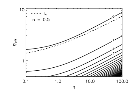
Figure 1: Critical value for shock formation of dimensionless orbital separation $\eta=d/R_{1}$ against mass ratio $q=M_{2}/M_{1}$. This applies for a circular orbit, the polytropic equation of state with $n=1/2$ ($\Gamma=3$), and $l=m=2$ perturbations. The labels $0,1,2,\dots$ denote the number of radial nodes in the mode. The critical value of $\eta$ for Roche lobe overflow through the Lagrange point $L_{1}$ is shown as a dashed line. At large $q$, $\eta\propto q^{1/3}$ for all curves.

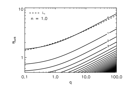
Figure 2: The same plots for the polytropic equation of state with $n=1$ ($\Gamma=2$).

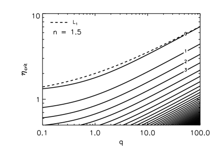
Figure 3: The same plots for the polytropic equation of state with $n=3/2$ ($\Gamma=5/3$).

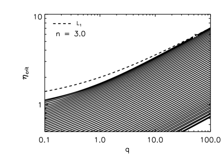
Figure 4: The same plots for the polytropic equation of state with $n=3$ ($\Gamma=4/3$). (The bottom right corner appears blank because we have not calculated modes there. All our figures show the same ranges of $\eta$ and $q$.)

5 Conclusions

This paper consists of two parts: a quantitative criterion for linear perturbation modes to form shocks, and an application of this criterion to modes raised by tidal forces in compact binaries.

Our shock formation criterion relies on the hodograph transformation to link linear perturbation modes in the interior to the fully nonlinear shock formation criterion of Gundlach & Please (2009) near the surface. This criterion is exact for plane-symmetric motion of a polytropic fluid in a constant gravitational field. The approximation of planar symmetry near the surface is natural, and it turns out that any buoyancy (non-barotropic) effects can also be safely neglected near the surface as long as the entropy gradient and any composition gradients are merely bounded.

Our calculation of the tidal waves in perturbation theory is straightforward for circular orbits (Lai (1994)). For stars with a simple polytropic equation of state $P=K\rho^{1+1/n}$ in irrotational circular binary orbit, we find that the critical orbital separation for shock formation essentially coincides with the one for Roche lobe overflow. In other words, tidal forces create shocks roughly when the binary begins to merge. Within our approximations, the two curves agree remarkably closely, so that we cannot say which actually occurs first. In any case, the $p$-mode shock formation mechanism we have investigated here is not the primary mechanism for binary disruption. As discussed above in Sec. 3.4, we expect the same result even for highly elliptic orbits. Although this is a negative result, it should be stressed that it was not obvious from dimensional analysis: we have also estimated the dimensionless factors.

Extending our analysis to more realistic stellar models would require more extensive modelling, in particular a realistic treatment of the surface. (We have shown above in Sec. 2.2 that another simple stellar model, assuming one polytropic constant for the equation of state and another for the stellar structure, gives rise to a divergent Brunt-Väisälä frequency, and so is inconsistent with our assumptions of a perfect fluid surface). However, the fact that our result holds for a polytropic index ranging from $n=1/2$ to $n=3$ suggests that other equations of state would not show shock formation before merger either. Intuitively, the weakness of the shock formation mechanism is dominated by a factor of (tidal force frequency/mode frequency$)^{2}$ [the factor $\sigma_{f}^{2}$ in Eq. (62)].

In a related result, Rosswog et al. (2009) give a criterion for the tidal disruption of a WD in orbit around a much more massive compact object 2 (black hole or NS) as (in our notation) $\eta_{\rm disrupt}\simeq q^{1/3}$ based on numerical simulations. Our results are consistent with this for large $q$ in that both Roche lobe overflow and tidal shock formation occur at the same $\eta$, namely $\eta_{\rm crit}\simeq 1.44q^{1/3}$ for $q\gg 1$.

Finally, this paper is motivated by the observance of surface shocks in numerical simulations of binary neutron star mergers just before the stars touch (Baiotti et al. (2008); Rezzolla et al. (2010)). Our results indicate that these surface shocks are probably not physical.

References

- Baiotti et al. (2008) Baiotti L., Giacomazzi B., Rezzolla L., 2008, Phys. Rev. D, 78, 084033.
- Bildsten & Cutler (1992) Bildsten L., Cutler C., 1992, AJ, 400, 175.
- Christensen-Dalsgaard (1997) Christensen-Dalsgaard J., 1997, code from http://astro.phys.au.dk/jcd/adipack.n/ (accessed in 2010)
- Christensen-Dalsgaard & Mullan (1994) Christensen-Dalsgaard J., Mullan D. J., 1994, MNRAS, 270, 921.
- Christensen-Dalsgaard et al (1996) Christensen-Dalsgaard J. et al, 1996, Sci, 272, 1286.
- Cox (1980) Cox J. P., 1980, Theory of stellar perturbations, Princeton University Press, Princeton.
- Dimmelmeyer et al. (2004) Dimmelmeyer H., Stergioulas N., Font J. A., 2004, MNRAS, 352, 1089.
- Gabler et al. (2009) Gabler M., Sperhake U., Andersson N., 2009, Phys. Rev. D, 80, 064012.
- Gundlach & Please (2009) Gundlach C., Please C. P., 2009, Phys. Rev. D, 79, 067501.
- Gundlach & LeVeque (2011) Gundlach C., LeVeque R. J., 2011, J. Fluid. Mech., in press.
- Kochanek (1992) Kochanek C. S., 1992, AJ, 398, 234.
- Lai (1994) Lai D., 1994, MNRAS 270, 611.
- Rezzolla et al. (2010) Rezzolla L. et al, 2010, Class. Quantum Grav., 27, 114105.
- Rosswog et al. (2009) Rosswog S., Ramirez-Ruiz E., Hix W. R., 2009, AJ, 695, 404.
- Shapiro & Teukolsky (2004) Shapiro S. L., Teukolsky S. A., 2004, Black holes, white dwarfs and neutron stars, Wiley, Weinheim.
- Stergioulas et al. (2006) Stergioulas N., Apostolatos T. A., Font J. A., 2006, MNRAS, 368, 1609.
- Unno et al. (1989) Unno W. et al., 1989, Nonradial oscillations of stars, 2nd edition, University of Tokyo Press, Tokyo.