Sufficient Component Analysis for Supervised Dimension Reduction

Abstract

The purpose of sufficient dimension reduction (SDR) is to find the low-dimensional subspace of input features that is sufficient for predicting output values. In this paper, we propose a novel distribution-free SDR method called sufficient component analysis (SCA), which is computationally more efficient than existing methods. In our method, a solution is computed by iteratively performing dependence estimation and maximization: Dependence estimation is analytically carried out by recently-proposed least-squares mutual information (LSMI), and dependence maximization is also analytically carried out by utilizing the Epanechnikov kernel. Through large-scale experiments on real-world image classification and audio tagging problems, the proposed method is shown to compare favorably with existing dimension reduction approaches.

1 Introduction

The goal of sufficient dimension reduction (SDR) is to learn a transformation matrix ${\bm{W}}$ from input feature ${\bm{x}}$ to its low-dimensional representation ${\bm{z}}$ ($={\bm{W}}{\bm{x}}$) which has ‘sufficient’ information for predicting output value ${\bm{y}}$. SDR can be formulated as the problem of finding ${\bm{z}}$ such that ${\bm{x}}$ and ${\bm{y}}$ are conditionally independent given ${\bm{z}}$ (Cook, 1998; Fukumizu et al., 2009).

Earlier SDR methods developed in statistics community, such as sliced inverse regression (Li, 1991), principal Hessian direction (Li, 1992), and sliced average variance estimation (Cook, 2000), rely on the elliptical assumption (e.g., Gaussian) of the data, which may not be fulfilled in practice.

To overcome the limitations of these approaches, the kernel dimension reduction (KDR) was proposed (Fukumizu et al., 2009). KDR employs a kernel-based dependence measure, which does not require the elliptical assumption (i.e., distribution-free), and the solution ${\bm{W}}$ is computed by a gradient method. Although KDR is a highly flexible SDR method, its critical weakness is the kernel function choice—the performance of KDR depends on the choice of kernel functions and the regularization parameter, but there is no systematic model selection method available. Furthermore, KDR scales poorly to massive datasets since the gradient-based optimization is computationally demanding. Another important limitation of KDR in practice is that there is no good way to set an initial solution—many random restarts may be needed for finding a good local optima, which makes the entire procedure even slower and the performance of dimension reduction unstable.

To overcome the limitations of KDR, a novel SDR method called least-squares dimension reduction (LSDR) was proposed recently (Suzuki & Sugiyama, 2010). LSDR adopts a squared-loss variant of mutual information as a dependency measure, which is efficiently estimated by least-squares mutual information (LSMI) (Suzuki et al., 2009). A notable advantage of LSDR over KDR is that kernel functions and its tuning parameters such as the kernel width and the regularization parameter can be naturally optimized by cross-validation. However, LSDR still relies on a computationally expensive gradient method and there is no good initialization scheme.

In this paper, we propose a novel SDR method called sufficient component analysis (SCA), which can overcome the computational inefficiency of LSDR. In SCA, the solution ${\bm{W}}$ in each iteration is obtained analytically by just solving an eigenvalue problem, which significantly contributes to improving the computational efficiency. Moreover, based on the above analytic-form solution, we develop a method to design a good initial value for optimization, which further reduces the computational cost and help obtain a good local optimum solution.

Through large-scale experiments using the PASCAL Visual Object Classes (VOC) 2010 dataset (Everingham et al., 2010) and the Freesound dataset (The Freesound Project, 2011), we demonstrate the usefulness of the proposed method.

2 Sufficient Dimension Reduction with Squared-Loss Mutual Information

In this section, we formulate the problem of sufficient dimension reduction (SDR) based on squared-loss mutual information (SMI).

2.1 Problem Formulation

Let ${\mathcal{X}}(\subset\mathbb{R}^{d})$ be the domain of input feature ${\bm{x}}$ and ${\mathcal{Y}}$ be the domain of output data ${\bm{y}}$. Suppose we are given $n$ independent and identically distributed (i.i.d.) paired samples,

$$D^{n}=\{({\bm{x}}_{i},{\bm{y}}_{i})~{}|~{}{\bm{x}}_{i}\in{\mathcal{X}},~{}{\bm{y}}_{i}\in{\mathcal{Y}},~{}i=1,\ldots,n\},$$

drawn from a joint distribution with density $p_{\mathrm{xy}}({\bm{x}},{\bm{y}})$.

The goal of SDR is to find a low-dimensional representation ${\bm{z}}$ ($\in\mathbb{R}^{m}$, $m\leq d$) of input ${\bm{x}}$ that is sufficient to describe output ${\bm{y}}$. More precisely, we find ${\bm{z}}$ such that

$${\bm{y}}\mathop{\perp\!\!\!\perp}{\bm{x}}~{}|~{}{\bm{z}},$$ (1)

meaning that, given the projected feature ${\bm{z}}$, the feature ${\bm{x}}$ is conditionally independent of output ${\bm{y}}$.

In this paper, we focus on linear dimension reduction scenarios:

$${\bm{z}}={\bm{W}}{\bm{x}},$$

where ${\bm{W}}$ is a transformation matrix. ${\bm{W}}$ belongs to the Stiefel manifold $\mathbb{S}_{m}^{d}(\mathbb{R})$:

$$\mathbb{S}_{m}^{d}(\mathbb{R}):=\{{\bm{W}}\in\mathbb{R}^{m\times d}|{\bm{W}}{\bm{W}}^{\top}={\bm{I}}_{m}\},$$

where ^⊤ denotes the transpose and ${\bm{I}}_{m}$ is the $m$-dimensional identity matrix. Below, we assume that the reduced dimension $m$ is known.

2.2 Dependence Estimation-Maximization Framework

Suzuki & Sugiyama (2010) showed that the optimal transformation matrix that leads to Eq.(1) can be characterized as

$${\bm{W}}^{\ast} =\mathop{\textnormal{argmax}}_{{\bm{W}}\in\mathbb{R}^{m\times d}}~{}\textnormal{SMI}(Z,Y)~{}~{}\text{s.t.}~{}{\bm{W}}{\bm{W}}^{\top}={\bm{I}}_{m}.$$ (2)

In the above, ${\mathrm{SMI}}(Z,Y)$ is the squared-loss mutual information:

$${\mathrm{SMI}}(Z,Y) :=\frac{1}{2}\mathbb{E}_{p_{\mathrm{z}},p_{\mathrm{y}}}\left[\left(\frac{p_{\mathrm{zy}}({\bm{z}},{\bm{y}})}{p_{\mathrm{y}}({\bm{y}})p_{\mathrm{z}}({\bm{z}})}-1\right)^{2}\right],$$

where $\mathbb{E}_{p_{\mathrm{z}},p_{\mathrm{y}}}$ denotes the expectation over the marginals $p_{\mathrm{z}}({\bm{z}})$ and $p_{\mathrm{y}}({\bm{y}})$. Note that SMI is the Pearson divergence from $p_{\mathrm{zy}}({\bm{z}},{\bm{y}})$ to $p_{\mathrm{z}}({\bm{z}})p_{\mathrm{y}}({\bm{y}})$, while the ordinary mutual information is the Kullback-Leibler divergence from $p_{\mathrm{zy}}({\bm{z}},{\bm{y}})$ to $p_{\mathrm{z}}({\bm{z}})p_{\mathrm{y}}({\bm{y}})$. The Pearson divergence and the Kullback-Leibler divergence both belong to the class of $f$-divergences, which shares similar theoretical properties. For example, SMI is non-negative and is zero if and only if $Z$ and $Y$ are statistically independent, as ordinary mutual information.

Based on Eq.(2), we develop the following iterative algorithm for learning ${\bm{W}}$:

(i) Initialization:

Initialize the transformation matrix ${\bm{W}}$ (see Section 3.3).

(ii) Dependence estimation:

For current ${\bm{W}}$, an SMI estimator $\widehat{\textnormal{SMI}}$ is obtained (see Section 3.1).

(iii) Dependence maximization:

Given an SMI estimator $\widehat{\textnormal{SMI}}$, its maximizer with respect to ${\bm{W}}$ is obtained (see Section 3.2).

(iv) Convergence check:

The above (ii) and (iii) are repeated until ${\bm{W}}$ fulfills some convergence criterion.

3 Proposed Method: Sufficient Component Analysis

In this section, we describe our proposed method called the sufficient component analysis (SCA).

3.1 Dependence Estimation

In SCA, we utilize a non-parametric SMI estimator called least-squares mutual information (LSMI) (Suzuki et al., 2009), which was shown to achieve the optimal convergence rate (Suzuki & Sugiyama, 2010). Here, we review LSMI.

3.1.1 Basic Idea

A key idea of LSMI is to directly estimate the density ratio,

$$w({\bm{z}},{\bm{y}})=\frac{p_{\mathrm{zy}}({\bm{z}},{\bm{y}})}{p_{\mathrm{z}}({\bm{z}})p_{\mathrm{y}}({\bm{y}})},$$

without going through density estimation of $p_{\mathrm{zy}}({\bm{z}},{\bm{y}})$, $p_{\mathrm{z}}({\bm{z}})$, and $p_{\mathrm{y}}({\bm{y}})$. Here, the density ratio function $w({\bm{z}},{\bm{y}})$ is directly modeled by

$$w_{{\bm{\alpha}}}({\bm{z}},{\bm{y}})=\sum_{\ell=1}^{n}\alpha_{\ell}K({\bm{z}},{\bm{z}}_{\ell})L({\bm{y}},{\bm{y}}_{\ell}),$$ (3)

where $K({\bm{z}},{\bm{z}}^{\prime})$ and $L({\bm{y}},{\bm{y}}^{\prime})$ are kernel functions for ${\bm{z}}$ and ${\bm{y}}$, respectively.

Then, the parameter ${\bm{\alpha}}=(\alpha_{1},\ldots,\alpha_{n})^{\top}$ is learned so that the following squared error is minimized:

$$J_{0}({\bm{\alpha}})=\frac{1}{2}\mathbb{E}_{p_{\mathrm{z}},p_{\mathrm{y}}}\left[(w_{{\bm{\alpha}}}({\bm{z}},{\bm{y}})-w({\bm{z}},{\bm{y}}))^{2}\right].$$

$J_{0}$ can be expressed as

$$J_{0}({\bm{\alpha}})=J({\bm{\alpha}})+\textnormal{SMI}(Z,Y)+\frac{1}{2},$$

where

$$J({\bm{\alpha}}) =\frac{1}{2}{\bm{\alpha}}^{\top}{\bm{H}}{\bm{\alpha}}-{\bm{h}}^{\top}{\bm{\alpha}},$$

$$H_{\ell,\ell^{\prime}} =\mathbb{E}_{p_{\mathrm{z}},p_{\mathrm{y}}}\left[K({\bm{z}},{\bm{z}}_{\ell})L({\bm{y}},{\bm{y}}_{\ell})K({\bm{z}},{\bm{z}}_{\ell^{\prime}})L({\bm{y}},{\bm{y}}_{\ell^{\prime}})\right],$$

$$h_{\ell} =\mathbb{E}_{p_{\mathrm{zy}}}\left[K({\bm{z}},{\bm{z}}_{\ell})L({\bm{y}},{\bm{y}}_{\ell})\right],$$

and $\textnormal{SMI}(Z,Y)$ is constant with respect to ${\bm{\alpha}}$. Thus, minimizing $J_{0}$ is equivalent to minimizing $J$.

3.1.2 Computing the Solution

Approximating the expectations in ${\bm{H}}$ and ${\bm{h}}$ included in $J$ by empirical averages, we arrive at the following optimization problem:

$$\min_{{\bm{\alpha}}}\left[\frac{1}{2}{\bm{\alpha}}^{\top}\widehat{{\bm{H}}}{\bm{\alpha}}-\widehat{{\bm{h}}}^{\top}{\bm{\alpha}}+\lambda{\bm{\alpha}}^{\top}{\bm{R}}{\bm{\alpha}}\right],$$

where a regularization term $\lambda{\bm{\alpha}}^{\top}{\bm{R}}{\bm{\alpha}}$ is included for avoiding overfitting, $\lambda$ ($\geq 0$) is a regularization parameter, ${\bm{R}}$ is a regularization matrix, and, for ${\bm{z}}_{i}={\bm{W}}{\bm{x}}_{i}$,

$$\widehat{H}_{\ell,\ell^{\prime}} =\frac{1}{n^{2}}\sum_{i,j=1}^{n}K({\bm{z}}_{i},{\bm{z}}_{\ell})L({\bm{y}}_{i},{\bm{y}}_{\ell})K({\bm{z}}_{j},{\bm{z}}_{\ell^{\prime}})L({\bm{y}}_{j},{\bm{y}}_{\ell^{\prime}}),$$

$$\widehat{h}_{\ell} =\frac{1}{n}\sum_{i=1}^{n}K({\bm{z}}_{i},{\bm{z}}_{\ell})L({\bm{y}}_{i},{\bm{y}}_{\ell}).$$

Differentiating the above objective function with respect to ${\bm{\alpha}}$ and equating it to zero, we can obtain an analytic-form solution:

$$\widehat{{\bm{\alpha}}}=(\widehat{{\bm{H}}}+\lambda{\bm{R}})^{-1}\widehat{{\bm{h}}}.$$ (4)

Based on the fact that ${\mathrm{SMI}}(Z,Y)$ is expressed as

$${\mathrm{SMI}}(Z,Y)=\frac{1}{2}\mathbb{E}_{p_{\mathrm{zy}}}\left[w({\bm{z}},{\bm{y}})\right]-\frac{1}{2},$$

the following SMI estimator can be obtained:

$$\widehat{\mathrm{SMI}} =\frac{1}{2}{\widehat{{\bm{h}}}}^{\top}\widehat{{\bm{\alpha}}}-\frac{1}{2}.$$ (5)

3.1.3 Model Selection

Hyper-parameters included in the kernel functions and the regularization parameter can be optimized by cross-validation with respect to $J$.

More specifically, the samples ${\mathcal{Z}}=\{({\bm{z}}_{i},{\bm{y}}_{i})\}_{i=1}^{n}$ are divided into $K$ disjoint subsets $\{{\mathcal{Z}}_{k}\}_{k=1}^{K}$ of (approximately) the same size. Then, an estimator $\widehat{{\bm{\alpha}}}_{{\mathcal{Z}}_{k}}$ is obtained using ${\mathcal{Z}}\backslash{\mathcal{Z}}_{k}$ (i.e,. all samples without ${\mathcal{Z}}_{k}$), and the approximation error for the hold-out samples ${\mathcal{Z}}_{k}$ is computed as

$$J_{{\mathcal{Z}}_{k}}^{(K\text{-CV})}=\frac{1}{2}\widehat{{\bm{\alpha}}}_{{\mathcal{Z}}_{k}}^{\top}\widehat{{\bm{H}}}_{{\mathcal{Z}}_{k}}\widehat{{\bm{\alpha}}}_{{\mathcal{Z}}_{k}}-\widehat{{\bm{h}}}_{{\mathcal{Z}}_{k}}^{\top}\widehat{{\bm{\alpha}}}_{{\mathcal{Z}}_{k}},$$

where, for $|{\mathcal{Z}}_{k}|$ being the number of samples in the subset ${\mathcal{Z}}_{k}$,

$$[\widehat{H}_{{\mathcal{Z}}_{k}}]_{\ell,\ell^{\prime}} =\frac{1}{|{\mathcal{Z}}_{k}|^{2}}\sum_{({\bm{z}},{\bm{y}}),({\bm{z}}^{\prime},{\bm{y}}^{\prime})\in{\mathcal{Z}}_{k}}K({\bm{z}},{\bm{z}}_{\ell})L({\bm{y}},{\bm{y}}_{\ell})$$

$$~{}~{}~{}~{}~{}~{}~{}~{}~{}~{}~{}~{}~{}\times K({\bm{z}}^{\prime},{\bm{z}}_{\ell^{\prime}})L({\bm{y}}^{\prime},{\bm{y}}_{\ell^{\prime}}),$$

$$[\widehat{h}_{{\mathcal{Z}}_{k}}]_{\ell} =\frac{1}{|{\mathcal{Z}}_{k}|}\sum_{({\bm{z}},{\bm{y}})\in{\mathcal{Z}}_{k}}K({\bm{z}},{\bm{z}}_{\ell})L({\bm{y}},{\bm{y}}_{\ell}).$$

This procedure is repeated for $k=1,\ldots,K$, and its average $J^{(K\text{-CV})}$ is outputted as

$$J^{(K\text{-CV})}=\frac{1}{K}\sum_{k=1}^{K}J_{{\mathcal{Z}}_{k}}^{(K\text{-CV})}.$$

We compute $J^{(K\text{-CV})}$ for all model candidates, and choose the model that minimizes $J^{(K\text{-CV})}$.

3.2 Dependence Maximization

Given an SMI estimator $\widehat{\mathrm{SMI}}$ (5), we next show how $\widehat{\mathrm{SMI}}$ can be efficiently maximized with respect to ${\bm{W}}$:

$$\max_{{\bm{W}}\in\mathbb{R}^{m\times d}}\widehat{\mathrm{SMI}}~{}~{}~{}\textnormal{s.t.}~{}{\bm{W}}{\bm{W}}^{\top}={\bm{I}}_{m}.$$

We propose to use a truncated negative quadratic function called the Epanechnikov kernel (Epanechnikov, 1969) as a kernel for ${\bm{z}}$:

$$K({\bm{z}},{\bm{z}}_{\ell}) =\max\left(0,1-\frac{\|{\bm{z}}-{\bm{z}}_{\ell}\|^{2}}{2\sigma_{\mathrm{z}}^{2}}\right).$$

Let $I(c)$ be the indicator function, i.e., $I(c)=1$ if $c$ is true and zero otherwise. Then, for the above kernel, $\widehat{\mathrm{SMI}}$ can be expressed as

$$\widehat{\mathrm{SMI}}=\frac{1}{2}{\textnormal{tr}}\left({\bm{W}}{\bm{D}}{\bm{W}}^{\top}\right)-\frac{1}{2},$$

where $\textnormal{tr}({\bm{A}})$ is the trace of matrix ${\bm{A}}$, and

$${\bm{D}} =\frac{1}{n}\sum_{i=1}^{n}\sum_{\ell=1}^{n}\widehat{\alpha}_{\ell}({\bm{W}})I\left(\frac{\|{\bm{W}}{\bm{x}}_{i}-{\bm{W}}{\bm{x}}_{\ell}\|^{2}}{2\sigma_{\mathrm{z}}^{2}}<1\right)$$

$$~{}~{}~{}\times L({\bm{y}}_{i},{\bm{y}}_{\ell})\left[\frac{1}{m}{\bm{I}}_{d}-\frac{1}{2\sigma_{\mathrm{z}}^{2}}({\bm{x}}_{i}-{\bm{x}}_{\ell})({\bm{x}}_{i}-{\bm{x}}_{\ell})^{\top}\right].$$

Here, by $\widehat{\alpha}_{\ell}({\bm{W}})$, we explicitly indicated the fact that $\widehat{\alpha}_{\ell}$ depends on ${\bm{W}}$.

Let ${\bm{D}}^{\prime}$ be ${\bm{D}}$ with ${\bm{W}}$ replaced by ${\bm{W}}^{\prime}$, where ${\bm{W}}^{\prime}$ is a transformation matrix obtained in the previous iteration. Thus, ${\bm{D}}^{\prime}$ no longer depends on ${\bm{W}}$. Here we replace ${\bm{D}}$ in $\widehat{\mathrm{SMI}}$ by ${\bm{D}}^{\prime}$, which gives the following simplified SMI estimate:

$$\frac{1}{2}{\textnormal{tr}}\left({\bm{W}}{\bm{D}}^{\prime}{\bm{W}}^{\top}\right)-\frac{1}{2}.$$ (6)

A maximizer of Eq.(6) can be analytically obtained by $({\bm{w}}_{1}|\cdots|{\bm{w}}_{m})^{\top}$, where $\{{\bm{w}}_{i}\}_{i=1}^{m}$ are the $m$ principal components of ${\bm{D}}^{\prime}$.

3.3 Initialization of ${\bm{W}}$

In the dependence estimation-maximization framework described in Section 2.2, initialization of the transformation matrix ${\bm{W}}$ is important. Here we propose to initialize it based on dependence maximization without dimensionality reduction.

More specifically, we determine the initial transformation matrix as $({\bm{w}}_{1}^{(0)}|\cdots|{\bm{w}}_{m}^{(0)})^{\top}$, where $\{{\bm{w}}_{i}^{(0)}\}_{i=1}^{m}$ are the $m$ principal components of ${\bm{D}}^{(0)}$:

$${\bm{D}}^{(0)} =\frac{1}{n}\sum_{i=1}^{n}\sum_{\ell=1}^{n}\widehat{\alpha}_{\ell}^{(0)}I\left(\frac{\|{\bm{x}}_{i}-{\bm{x}}_{\ell}\|^{2}}{2\sigma_{\mathrm{x}}^{2}}<1\right)L({\bm{y}}_{i},{\bm{y}}_{\ell})$$

$$~{}~{}~{}\times\left[\frac{1}{m}{\bm{I}}_{d}-\frac{1}{2\sigma_{\mathrm{x}}^{2}}({\bm{x}}_{i}-{\bm{x}}_{\ell})({\bm{x}}_{i}-{\bm{x}}_{\ell})^{\top}\right],$$

$$\widehat{{\bm{\alpha}}}^{(0)} =(\widehat{{\bm{H}}}^{(0)}+\lambda{\bm{R}})^{-1}\widehat{{\bm{h}}}^{(0)},$$

$$\widehat{H}^{(0)}_{\ell,\ell^{\prime}} =\frac{1}{n^{2}}\sum_{i,j=1}^{n}K^{\prime}({\bm{x}}_{i},{\bm{x}}_{\ell})L({\bm{y}}_{i},{\bm{y}}_{\ell})$$

$$~{}~{}~{}~{}~{}~{}~{}\times K^{\prime}({\bm{x}}_{j},{\bm{x}}_{\ell^{\prime}})L({\bm{y}}_{j},{\bm{y}}_{\ell^{\prime}}),$$

$$\widehat{h}^{(0)}_{\ell} =\frac{1}{n}\sum_{i=1}^{n}K^{\prime}({\bm{x}}_{i},{\bm{x}}_{\ell})L({\bm{y}}_{i},{\bm{y}}_{\ell}),$$

$$K^{\prime}({\bm{x}},{\bm{x}}_{\ell}) =\max\left(0,1-\frac{\|{\bm{x}}-{\bm{x}}_{\ell}\|^{2}}{2\sigma_{\mathrm{x}}^{2}}\right).$$

$\sigma_{{\mathrm{x}}}$ is the kernel width and is chosen by cross-validation (see Section 3.1.3).

4 Relation to Existing Methods

Here, we review existing SDR methods and discuss the relation to the proposed SCA method.

4.1 Kernel Dimension Reduction

Kernel Dimension Reduction (KDR) (Fukumizu et al., 2009) tries to directly maximize the conditional independence of ${\bm{x}}$ and ${\bm{y}}$ given ${\bm{z}}$ under a kernel-based independence measure.

The KDR learning criterion is given by

$${{\bm{W}}}^{\ast} =\mathop{\textnormal{argmax}}_{{\bm{W}}\in\mathbb{R}^{m\times d}}\textnormal{tr}\left[\widetilde{{\bm{L}}}(\widetilde{{\bm{K}}}+n\epsilon{\bm{I}}_{n})^{-1}\right]$$

$$~{}~{}~{}~{}~{}\text{s.t.}~{}{\bm{W}}{\bm{W}}^{\top}={\bm{I}}_{m},$$ (7)

where $\widetilde{{\bm{L}}}={\bm{\Gamma}}{\bm{L}}{\bm{\Gamma}}$, ${\bm{\Gamma}}={\bm{I}}-\frac{1}{n}{\bm{1}}_{n}{\bm{1}}_{n}^{\top}$, $L_{i,j}=L({\bm{y}}_{i},{\bm{y}}_{j})$, $\widetilde{{\bm{K}}}={\bm{\Gamma}}{\bm{K}}{\bm{\Gamma}}$, $K_{i,j}=K({\bm{z}}_{i},{\bm{z}}_{j})$, and $\epsilon$ is a regularization parameter.

Solving the above optimization problem is cumbersome since the objective function is non-convex. In the original KDR paper (Fukumizu et al., 2009), a gradient method is employed for finding a local optimal solution. However, the gradient-based optimization is computationally demanding due to its slow convergence and it requires many restarts for finding a good local optima. Thus, KDR scales poorly to massive datasets.

Another critical weakness of KDR is the kernel function choice. The performance of KDR depends on the choice of kernel functions and the regularization parameter, but there is no systematic model selection method for KDR available. Using the Gaussian kernel with its width set to the median distance between samples is a standard heuristic in practice, but this does not always work very well.

Furthermore, KDR lacks a good way to set an initial solution in the gradient procedure. Then, in practice, we need to run the algorithm many times with random initial points for finding good local optima. However, this makes the entire procedure even slower and the performance of dimension reduction unstable.

The proposed SCA method can successfully overcome the above weaknesses of KDR—SCA is equipped with cross-validation for model selection (Section 3.1.3), its solution can be computed analytically (see Section 3.2), and a systematic initialization scheme is available (see Section 3.3).

4.2 Least-Squares Dimensionality Reduction

Least-squares dimension reduction (LSDR) is a recently proposed SDR method that can overcome the limitations of KDR (Suzuki & Sugiyama, 2010). That is, LSDR is equipped with a natural model selection procedure based on cross-validation.

The proposed SCA can actually be regarded as a computationally efficient alternative to LSDR. Indeed, LSDR can also be interpreted as a dependence estimation-maximization algorithm (see Section 2.2), and the dependence estimation procedure is essentially the same as the proposed SCA, i.e., LSMI is used. The dependence maximization procedure is different from SCA—LSDR uses a natural gradient method (Amari, 1998).

In LSDR, the following SMI estimator is used:

$$\widetilde{\textnormal{SMI}}=\widehat{{\bm{\alpha}}}^{\top}{\widehat{{\bm{h}}}}-\frac{1}{2}\widehat{{\bm{\alpha}}}^{\top}{\widehat{{\bm{H}}}}\widehat{{\bm{\alpha}}}-\frac{1}{2},$$

where $\widehat{{\bm{\alpha}}}$, ${\widehat{{\bm{h}}}}$ and ${\widehat{{\bm{H}}}}$ are defined in Section 3.1. Then the gradient of $\widetilde{\textnormal{SMI}}$ is given by

$$\frac{\partial\widetilde{\textnormal{SMI}}}{\partial W_{\ell,\ell^{\prime}}} =\frac{\partial\widehat{{\bm{h}}}^{\top}}{\partial W_{\ell,\ell^{\prime}}}(2\widehat{{\bm{\alpha}}}-{\widehat{{\bm{\beta}}}})-\widehat{{\bm{\alpha}}}^{\top}\frac{\partial\widehat{{\bm{H}}}}{\partial W_{\ell,\ell^{\prime}}}(\frac{3}{2}\widehat{{\bm{\alpha}}}-{\widehat{{\bm{\beta}}}})$$

$$~{}~{}~{}~{}+\widehat{{\bm{\alpha}}}^{\top}\frac{\partial{\bm{R}}}{\partial W_{\ell,\ell^{\prime}}}({\widehat{{\bm{\beta}}}}-\widehat{{\bm{\alpha}}}),$$

where ${\widehat{{\bm{\beta}}}}=(\widehat{{\bm{H}}}+\lambda{\bm{R}})^{-1}\widehat{{\bm{H}}}\widehat{{\bm{\alpha}}}$. The natural gradient update of ${\bm{W}}$, which takes into account the structure of the Stiefel manifold (Amari, 1998), is given by

$${\bm{W}}\leftarrow{\bm{W}}\exp\left(\eta\Bigg{(}{\bm{W}}^{\top}\frac{\partial\widetilde{\textnormal{SMI}}}{\partial{\bm{W}}}-\frac{\partial\widetilde{\textnormal{SMI}}}{\partial{\bm{W}}}^{\top}{\bm{W}}\Bigg{)}\right),$$

where ‘$\exp$’ for a matrix denotes the matrix exponential. $\eta\geq 0$ is a step size, which may be optimized by a line-search method such as Armijo’s rule (Patriksson, 1999).

Since cross-validation is available for model selection of LSMI, LSDR is more favorable than KDR. However, its optimization still relies on a gradient-based method and thus it is computationally expensive.

Furthermore, there seems no good initialization scheme of the transformation matrix ${\bm{W}}$. In the original paper by Suzuki & Sugiyama (2010), initial values were chosen randomly and the gradient method was run many times for finding a better local solution.

The proposed SCA method can successfully overcome the above weaknesses of LSDR, by providing an analytic-form solution (see Section 3.2) and a systematic initialization scheme (see Section 3.3).

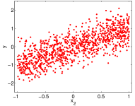
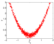
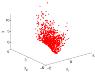
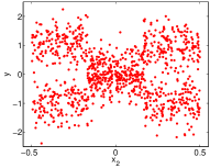
Figure 1: Artificial datasets.

Table 1: Mean of Frobenius-norm error (with standard deviations in brackets) and mean CPU time over 100 trials. Computation time is normalized so that LSDR is one. LSDR was repeated 5 times with random initialization and the transformation matrix with the minimum CV score was chosen as the final solution. ‘SCA(0)’ indicates the performance of the initial transformation matrix obtained by the method described in Section 3.3. The best method in terms of the mean Frobenius-norm and comparable methods according to the t-test at the significance level $1\%$ are specified by bold face.

Datasets	$d$	$m$	SCA(0)		SCA		LSDR		KDR		SIR		SAVE		pHd
Data1	4	1	.089	(.042)	.048	(.031)	.056	(.021)	.048	(.019)	.257	(.168)	.339	(.218)	.593	(.210)
Data2	10	1	.078	(.019)	.007	(.002)	.039	(.023)	.024	(.007)	.431	(.281)	.348	(.206)	.443	(.222)
Data3	4	2	.065	(.035)	.018	(.010)	.090	(.069)	.029	(.119)	.362	(.182)	.343	(.213)	.437	(.231)
Data4	5	1	.118	(.046)	.042	(.030)	.151	(.296)	.118	(.238)	.421	(.268)	.356	(.197)	.591	(.205)
Time			0.03		0.49		1.0		0.96		$<$0.01		$<$0.01		$<$0.01

5 Experiments

In this section, we experimentally investigate the performance of the proposed and existing SDR methods using artificial and real-world datasets.

5.1 Artificial Datasets

We use four artificial datasets, and compare the proposed SCA, LSDR (Suzuki & Sugiyama, 2010), KDR (Fukumizu et al., 2009), sliced inverse regression (SIR) (Li, 1991), sliced average variance estimation (SAVE)³ (Cook, 2000), and principal Hessian direction (pHd)³ (Li, 1992).

In SCA, we use the Gaussian kernel for ${\bm{y}}$:

$$L({\bm{y}},{\bm{y}}_{\ell})=\exp\left(-\frac{\|{\bm{y}}-{\bm{y}}_{\ell}\|^{2}}{2\sigma_{\mathrm{y}}}\right).$$

The identity matrix is used as regularization matrix ${\bm{R}}$, and the kernel widths $\sigma_{\mathrm{x}}$, $\sigma_{\mathrm{y}}$, and $\sigma_{\mathrm{z}}$ as well as the regularization parameter $\lambda$ are chosen based on 5-fold cross-validation.

The performance of each method is measured by

$$\frac{1}{\sqrt{2m}}\|\widehat{{\bm{W}}}^{\top}\widehat{{\bm{W}}}-{\bm{W}}^{\ast\top}{\bm{W}}^{\ast}\|_{\mathrm{Frobenius}},$$

where $\|\cdot\|_{\mathrm{Frobenius}}$ denotes the Frobenius norm, $\widehat{{\bm{W}}}$ is an estimated transformation matrix, and ${\bm{W}}^{\ast}$ is the optimal transformation matrix. Note that the above error measure takes its value in $[0,1]$.

We use the following four datasets (see Figure 1):

(a) Data1:

$$Y=X_{2}+0.5E,$$

where $(X_{1},\ldots,X_{4})^{\top}\sim U([-1~{}1]^{4})$ and $E\sim N(0,1)$. Here, $U({\mathcal{S}})$ denotes the uniform distribution on ${\mathcal{S}}$, and $N({\bm{\mu}},{\bm{\Sigma}})$ is the Gaussian distribution with mean ${\bm{\mu}}$ and variance ${\bm{\Sigma}}$.

(b) Data2:

$$Y=(X_{3})^{2}+0.1E,$$

where $(X_{1},\ldots,X_{10})^{\top}\sim N({\bm{0}}_{10},{\bm{I}}_{10})$ and $E\sim N(0,1)$.

(c) Data3:

$$Y=\frac{(X_{1})^{2}+X_{2}}{0.5+(X_{2}+1.5)^{2}}+(1+X_{2})^{2}+0.1E,$$

where $(X_{1},\ldots,X_{4})^{\top}\sim N({\bm{0}}_{4},{\bm{I}}_{4})$ and $E\sim N(0,1)$.

(d) Data4:

$$Y|X_{2}\sim\left\{\begin{array}[]{ll}N(0,0.2)&\textnormal{if}~{}X_{2}\leq|1/6|\\ 0.5N(1,0.2)&\textnormal{otherwise}\\ +0.5N(-1,0.2),\\ \end{array}\right.$$

where $(X_{1},\ldots,X_{5})^{\top}\sim U([-0.5~{}0.5]^{5})$ and $E\sim N(0,1)$.

The performance of each method is summarized in Table LABEL:table:toy, which depicts the mean and standard deviation of the Frobenius-norm error over 100 trials when the number of samples is $n=1000$. As can be observed, the proposed SCA overall performs well. ‘SCA(0)’ in the table indicates the performance of the initial transformation matrix obtained by the method described in Section 3.3. The result shows that SCA(0) gives a reasonably good transformation matrix with a tiny computational cost. Note that KDR and LSDR have high standard deviation for Data3 and Data4, meaning that KDR and LSDR sometimes perform poorly.

5.2 Multi-label Classification for Real-world Datasets

Finally, we evaluate the performance of the proposed method in real-world multi-label classification problems.

5.2.1 Setup

Below, we compare SCA, Multi-label Dimensionality reduction via Dependence Maximization (MDDM) (Zhang & Zhou, 2010), Canonical Correlation Analysis (CCA) (Hotelling, 1936), and Principal Component Analysis (PCA) (Bishop, 2006). We use a real-world image classification dataset called the PASCAL Visual Object Classes (VOC) 2010 dataset (Everingham et al., 2010) and a real-world automatic audio-tagging dataset called the Freesound dataset (The Freesound Project, 2011). Since the computational costs of KDR and LSDR were unbearably large, we decided not to include them in the comparison.

We employ the misclassification rate by the nearest-neighbor classifier as a performance measure:

$$\mathrm{err}=\frac{1}{nc}\sum_{i=1}^{n}\sum_{k=1}^{c}I(\widehat{y}_{i,k}\neq y_{i,k}),$$

where $c$ is the number of classes, $\widehat{y}$ and $y$ are the estimated and true labels, and $I(y\neq y^{\prime})$ is the indicator function.

For SCA and MDDM, we use the following kernel function (Sarwar et al., 2001) for ${\bm{y}}$:

$$L({\bm{y}},{\bm{y}}^{\prime})=\frac{({\bm{y}}-\overline{{\bm{y}}})^{\top}({\bm{y}}^{\prime}-\overline{{\bm{y}}})}{\|{\bm{y}}-\overline{{\bm{y}}}\|\|{\bm{y}}^{\prime}-\overline{{\bm{y}}}^{\prime}\|},$$

where $\overline{{\bm{y}}}$ is the sample mean: $\overline{{\bm{y}}}=\frac{1}{n}\sum_{i=1}^{n}{\bm{y}}_{i}$.

5.2.2 PASCAL VOC 2010 Dataset

The VOC 2010 dataset consists of 20 binary classification tasks of identifying the existence of a person, aeroplane, etc. in each image. The total number of images in the dataset is 11319, and we used 1000 randomly chosen images for training and the rest for testing.

In this experiment, we first extracted visual features from each image using the Speed Up Robust Features (SURF) algorithm (Bay et al., 2008), and obtained 500 visual words as the cluster centers in the SURF space. Then, we computed a 500-dimensional bag-of-feature vector by counting the number of visual words in each image. We randomly sampled the training and test data 100 times, and computed the means and standard deviations of the classification error.

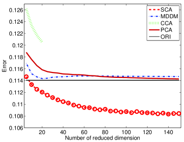
(a) VOC 2010 dataset

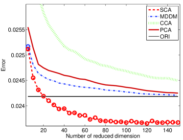
(b) Freesound dataset

Figure 2: Results on image classification with VOC 2010 dataset and audio classification with Freesound datasets. Misclassification rate when the one-nearest-neighbor classifier is used as a classifier is reported. The best dimension reduction method in terms of the mean error and comparable methods according to the t-test at the significance level 1% are specified by ‘$\circ$’. CCA can be applied to dimension reduction up to $c$ dimensions, where $c$ is the number of classes ($c=20$ in VOC 2010 and $c=230$ in Freesound). ‘ORI’ denotes the original data without dimension reduction.

The results are plotted in Figure 2(a), showing that SCA outperforms the existing methods, and SCA is the only method that outperforms ‘ORI’ (no dimension reduction)—SCA achieves almost the same error rate as ‘ORI’ with only a 10-dimensional subspace.

5.2.3 Freesound Dataset

The Freesound dataset (The Freesound Project, 2011) consists of various audio files annotated with word tags such as ‘people’, ‘noisy’, and ‘restaurant’. We used 230 tags in this experiment. The total number of audio files in the dataset is 5905, and we used 1000 randomly chosen audio files for training and the rest for testing.

We first extracted Mel-Frequency Cepstrum Coefficients (MFCC) (Rabiner & Juang, 1993) from each audio file, and obtained 1024 audio features as the cluster centers in MFCC. Then, we computed a 1024-dimensional bag-of-feature vector by counting the number of audio features in each audio file. We randomly chose the training and test samples 100 times, and computed the means and standard deviations of the classification error.

The results plotted in Figure 2(b) show that, similarly to the image classification task, the proposed SCA outperforms the existing methods, and SCA is the only method that outperforms ‘ORI’.

6 Conclusion

In this paper, we proposed a novel sufficient dimension reduction (SDR) method called sufficient component analysis (SCA), which is computationally more efficient than existing SDR methods. In SCA, a transformation matrix was estimated by iteratively performing dependence estimation and maximization, both of which are analytically carried out. Moreover, we developed a systematic method to design a good initial transformation matrix, which highly contributes to further reducing the computational cost and help obtain a good local optimum solution. We applied the proposed SCA to real-world image classification and audio tagging tasks, and experimentally showed that the proposed method is promising.

References

- Amari (1998) Amari, S. Natural gradient works efficiently in learning. Neural Computation, 10:251–276, 1998.
- Bay et al. (2008) Bay, H., Ess, A., Tuytelaars, T., and Gool, L. V. Surf: Speeded up robust features. Computer Vision and Image Understanding, 110(3):346–359, 2008.
- Bishop (2006) Bishop, C. M. Pattern Recognition and Machine Learning. Springer, New York, NY, 2006.
- Cook (1998) Cook, R. D. Regression graphics: Ideas for studying regressions through graphics. Wiley, New York, 1998.
- Cook (2000) Cook, R. D. Save: A method for dimension reduction and graphics in regression. Theory and Methods, 29:2109–2121, 2000.
- Epanechnikov (1969) Epanechnikov, V. Nonparametric estimates of a multivariate probability density. Theory of Probability and its Applications, 14:153–158, 1969.
- Everingham et al. (2010) Everingham, M., Gool, L. V., Williams, C. K. I., Winn, J., and Zisserman, A. The PASCAL Visual Object Classes Challenge 2010 (VOC2010) Results. http://www.pascal-network.org/challenges/VOC/voc2010/workshop/ index.html, 2010.
- Fukumizu et al. (2009) Fukumizu, K., Bach, F. R., and Jordan, M. Kernel dimension reduction in regression. The Annals of Statistics, 37(4):1871–1905, 2009.
- Hotelling (1936) Hotelling, H. Relations between two sets of variates. Biometrika, 28:321–377, 1936.
- Li (1991) Li, K.-C. Sliced inverse regression for dimension reduction. Journal of American Statistical Association, 86:316–342, 1991.
- Li (1992) Li, K.-C. On principal Hessian directions for data visualization and dimension reduction: Another application of Stein fs lemma. Journal of American Statistical Association, 87:1025–1034, 1992.
- Patriksson (1999) Patriksson, M. Nonlinear Programming and Variational Inequality Problems. Kluwer Academic, Dredrecht, 1999.
- Rabiner & Juang (1993) Rabiner, L. and Juang, B-H. Fundamentals of Speech Recognition. Prentice Hall, Englewood Cliffs, NJ, 1993.
- Sarwar et al. (2001) Sarwar, B., Karypis, G., Konstan, J., and Reidl, J. Item-based collaborative filtering recommendation algorithms. In Proceedings of the 10th international conference on World Wide Web (WWW2001), pp. 285–295, 2001.
- Suzuki & Sugiyama (2010) Suzuki, T. and Sugiyama, M. Sufficient dimension reduction via squared-loss mutual information estimation. In Proceedings of the Thirteenth International Conference on Artificial Intelligence and Statistics (AISTATS2010), pp. 804–811, 2010.
- Suzuki et al. (2009) Suzuki, T., Sugiyama, M., Kanamori, T., and Sese, J. Mutual information estimation reveals global associations between stimuli and biological processes. BMC Bioinformatics, 10(S52), 2009.
- The Freesound Project (2011) The Freesound Project. Freesound, 2011. http://www.freesound.org.
- Zhang & Zhou (2010) Zhang, Y. and Zhou, Z.-H. Multilabel dimensionality reduction via dependence maximization. ACM Trans. Knowl. Discov. Data, 4:14:1–14:21, 2010. ISSN 1556-4681.