Decay of currents for strong interactions

Abstract

The decay of current autocorrelation functions is investigated for quantum systems featuring strong ‘interactions’. Here, the term interaction refers to that part of the Hamiltonian causing the (major) decay of the current. On the time scale before the (first) zero-crossing of the current, its relaxation is shown to be well described by a suitable perturbation theory in the lowest orders of the interaction strength, even and especially if interactions are strong. In this description the relaxation is found to be rather close to a Gaussian decay and the resulting diffusion coefficient approximately scales with the inverse interaction strength. These findings are also confirmed by numerical results from exact diagonalization for several one-dimensional transport models including spin transport in the Heisenberg chain w.r.t. different spin quantum numbers, anisotropy, next-to-nearest-neighbor interaction, or alternating magnetic field; energy transport in the Ising chain with tilted magnetic field; and transport of excitations in a randomly coupled modular quantum system. The impact of these results for weak interactions is finally discussed.

I Introduction

Perturbation theory is one of the main approaches to many-particle physics with a wide range of applications in the context of quantum transport, ranging from the investigation of Green’s functions using Feynman graphs, the setup of a (quasi-)particle description by means of a Boltzmann equation, the derivation of the Green-Kubo formula within linear response theory kubo1991 ; mahan2000 , to many other applications in this context sirker2009 . A particular application is the use of different projection operator techniques nakajima1958 ; zwanzig1960 ; mori1965 ; forstner1975 ; chaturvedi1979 ; breuer2007 for the realization of steady-state bath scenarios mejiamonasterio2007 ; michel2008 ; prosen2009 ; steinigeweg2009-1 ; prosen2010 ; prosen2011 ; znidaric2011 or the analysis of current autocorrelations jung2006 ; jung2007 ; steinigeweg2010-2 . A perturbation theory is commonly employed due to the availability of a small parameter, e.g., weak particle-particle interactions, external scattering centers, or system-bath coupling. But additional assumptions are often required, such as the random phase and Markov approximation mahan2000 ; breuer2007 .
The concrete choice of a projection operator technique is a subtle task, whenever the addressed dynamics becomes non-Markovian and features memory effects steinigeweg2007 , typically occurring at short time scales. Because the relevant time scales are short in the case of strong perturbations, such non-Markovian effects appear in an already difficult case for any perturbation theory. However, the decay of the spin-current in the anisotropic Heisenberg chain zotos2003 ; heidrichmeisner2007 at high temperatures has been well described for the case of large anisotropy parameters in Ref. steinigeweg2010-2, by a lowest order prediction in the anisotropy, as obtained from a certain variant of projection operator techniques. Moreover, the resulting quantitative values for the diffusion coefficient have been brought into good agreement with numerical findings in the literature prelovsek2004 ; michel2008 ; prosen2009 ; huber1969-1 ; huber1969-2 ; karadamoglou2004 . But the perturbation theory in Ref. steinigeweg2010-2, has focused on a single quantum model so far and has been carried out numerically on the basis of finite systems solely, leaving the origin of the observed agreements and disagreements as an open issue. Hence, one main intention of this paper is the extension of the perturbation theory to a wider class of quantum models and the analytical treatment of strong perturbations in the thermodynamic limit (and weak perturbations close to that limit). Furthermore, criteria for the validity of the lowest order prediction will be formulated and higher order corrections will be taken into account. By the use of these criteria and the comparison with numerically exact diagonalization (ED) the relaxation of the current is found to be well described in the lowest orders of the perturbation, even and especially if the perturbation is not weak. In particular the relaxation is rather close to a Gaussian decay and the resulting diffusion coefficient roughly scales with the inverse perturbation strength.

This paper is structured as follows: In the next Sec. II the general definition of the current and the connection between its autocorrelation and the diffusion coefficient is briefly reviewed at first. Then the perturbation theory for the decay of the current autocorrelation is introduced in Sec. III and the validity of the lowest order truncation for strong perturbations is discussed in detail here. In the following Secs. IV-VI the introduced perturbation theory is applied to several one-dimensional transport models in the limit of high temperatures, namely, the transport of excitations in a randomly coupled modular quantum system (Sec. IV); spin transport in the Heisenberg chain w.r.t. anisotropy, next-to-nearest neighbor interactions, different spin quantum numbers, or a staggered magnetic field (Sec. V); and energy transport in the Ising chain with a tilted magnetic field (Sec. VI). The last Sec. VII closes with a summary and conclusion.

II Current and Diffusion Coefficient

In the present paper several (quasi-)one-dimensional and translationally invariant quantum systems will be studied, described by a respective Hamiltonian $H$. For such systems a globally conserved transport quantity $X$ will be considered, i.e., $[H,X]=0$. The latter quantity, and the Hamiltonian as well, are both decomposable into $N$ local portions $x_{r}$ and $h_{r}$, corresponding to different spatial positions $r$:

$$X=\sum_{r=1}^{N}x_{r}\,,\;H=\sum_{r=1}^{N}h_{r}\,.$$ (1)

Here, the $x_{r}$ may be defined either exactly on the position of the $h_{r}$, in between, or both. The above decomposition is further done in such a way that Heisenberg’s equation of motion is of the form ($\hbar\equiv 1$)

$$\frac{\text{d}}{\text{d}t}\,x_{r}=\imath[H,x_{r}] = \imath[h_{r^{-}},x_{r}]+\imath[h_{r^{+}},x_{r}]$$ (2)

$$\equiv j_{r-1}-j_{r}\,,$$

where $h_{r^{-}}$ and $h_{r^{+}}$ are located directly on the l.h.s. and r.h.s. of $x_{r}$, respectively. Because only the contributions from next neighbors $r^{-}$ and $r^{+}$ are involved, this form may require the choice of a proper elementary cell. For instance, if additional contributions from next-to-nearest neighbors occur, a larger cell consisting of two or even more sites may be chosen. However, once a description in terms of Eqs. (1) and (2) has been established, the local current is consistently defined by $j_{r}=\imath[x_{r},h_{r^{+}}]$ steinigeweg2009-3 and the total current reads

$$J=\sum_{r=1}^{N}j_{r}\,.$$ (3)

This paper will focus on the current autocorrelation function $C(t)=\langle J(t)J(0)\rangle$. Here, the time arguments of operators have to be understood w.r.t. the Heisenberg picture and the angles denote the equilibrium average at infinite temperature, i.e., essentially the trace operation: $\langle\ldots\rangle=\text{Tr}\{$…}$/\text{dim}{\cal H}$. Particularly, the time-integral

$${\cal D}(t)=\frac{1}{\langle X^{2}\rangle}\int_{0}^{t}\!\text{d}t^{\prime}\,C(t^{\prime})$$ (4)

will be of interest. Apparently, for $t\rightarrow\infty$, the quantity ${\cal D}(t)$ coincides with the diffusion constant according to linear response theory kubo1991 ; mahan2000 . However, for any finite time, this quantity is also connected to the actual expectation value of local densities

$$d_{r}(t)=\text{Tr}\{x_{r}(t)\rho(0)\}-\langle x_{r}\rangle\,,$$ (5)

where $\rho(0)$ represents an initial density matrix, featuring an inhomogeneous nonequilibrium density profile at the beginning. Concretely, the above quantity ${\cal D}(t)$ and the spatial variance

$$\text{Var}_{r}(t)=\sum_{r=1}^{N}d_{r}(t)\,r^{2}-\left[\sum_{r=1}^{N}d_{r}(t)\,r\right]^{2}$$ (6)

are connected via the relation steinigeweg2009-3

$$\frac{\text{d}}{\text{d}t}\,\text{Var}_{r}(t)=2\,{\cal D}(t)\,.$$ (7)

Thus, whenever ${\cal D}(t)$ is constant at a certain time scale, $\text{Var}_{r}(t)$ increases linearly at that scale, as expected for the case of diffusive dynamics. Contrary, ${\cal D}(t)=0$ yields no increase (insulating behavior) and ${\cal D}(t)\propto t$ leads to a quadratic increase (ballistic behavior).
Strictly speaking, the relation in Eq. (7) is only fulfilled exactly for a class of initial states $\rho(0)$ steinigeweg2009-3 , representing however an ensemble average w.r.t. typicality goldstein2006 ; popescu2006 ; reimann2007 or, more accurately, the dynamical typicality of quantum expectation values bartsch2009 . Hence, the overwhelming majority of all possible initial states $\rho(0)$ is nevertheless expected to yield roughly a spatial variance corresponding to the ensemble average, if only the dimension of the relevant Hilbert space is sufficiently large. The latter largeness is certainly satisfied for most practical purposes. In other words, a concrete initial state $\rho(0)$ is expected to fulfill approximately the relation in Eq. (7), at least if $\rho(0)$ is not constructed explicitly to violate this relation. Note that the relation in Eq. (7) remains still reasonable for lower temperatures, if all trace operations are performed including the statistical operator at a given temperature, see Ref. steinigeweg2009-3, for details.

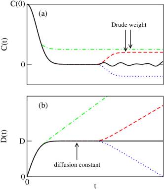
Figure 1: (color online) Sketch for the possible time-dependence of (a) the current autocorrelation function $C(t)$ and (b) its time-integral ${\cal D}(t)$. In (a) the current autocorrelation function $C(t)$ may decay completely at short times and then remain zero at intermediate times (black, solid curve). At long times $C(t)$ may decrease further to negative values (blue, dotted curve) or instead also increase to a positive value, due to a finite Drude weight (red, dashed curve). Such a Drude weight can already become dominant before the zero-crossing (green, dashed-dotted curve). In (b) the resulting time-integral ${\cal D}(t)$ may develop a plateau at intermediate times (black, solid curve), indicating diffusive dynamics. In that case the height of the latter plateau corresponds to the quantitative value of the diffusion constant $\cal D$. The width of this plateau, and its existence as such, both depend on the concrete form of the underlying current autocorrelation function in (a) (other curves).

Generally, the dynamical behavior crucially depends on the considered time scale. At sufficiently short times transport generically is ballistic: The time-integral ${\cal D}(t)$ firstly increases linearly, because the underlying current autocorrelation function $C(t)$ has not decayed yet, at least not significantly, see Fig. 1. But, if the current is not strictly conserved, its autocorrelation function $C(t)$ can further decay and may eventually reach a value close to zero at intermediate times. If $C(t)$ additionally remains at a value in the vicinity of zero, its time-integral ${\cal D}(t)$ approximately becomes constant and finally develops a plateau at such time scales, see Fig. 1. Then transport is diffusive and the respective diffusion coefficient is given by the height of the latter plateau. One main intention of this paper is to deduce the quantitative value of this diffusion coefficient perturbatively, especially in the case of strong perturbations, see the following Sec. III.
However, even if ${\cal D}(t)$ features a plateau at intermediate times, the dynamics does not necessarily stay diffusive for arbitrary long times. First, if the current is partially conserved, its autocorrelation function $C(t)$ contains a non-decaying contribution (finite Drude weight). Such a contribution, independent of its weight, eventually leads to a renewed linear increase of ${\cal D}(t)$ for sufficiently long times and consequently yields ballistic dynamics again, cf. Fig. 1 (red, dashed curve). Particularly, ${\cal D}(t)$ diverges for $t\rightarrow\infty$. The latter similarly happens, whenever the current autocorrelation function $C(t)$ is (quasi-)periodic in $t$ (finite recurrence time). But the renewed increase of ${\cal D}(t)$ in Fig. 1 (red, dashed curve) typically turns out to be a finite size effect, see Sec. V and Refs. steinigeweg2009-2, ; steinigeweg2010-2, .
Second, apart from transitions towards ballistic behavior in the limit of long times, transitions towards insulating behavior can appear, of course. In that case the current autocorrelation function $C(t)$ crosses zero and takes on a negative value, yielding a decrease of its time-integral ${\cal D}(t)$, see Fig. 1 (blue, dotted curve). However, all those transitions, occurring after a zero-crossing of the current, are not in the focus of this paper. In fact, the introduced perturbation theory in the following Section addresses the dynamics on the time scale before any occurrence of a zero-crossing. Strictly speaking, the theory itself does not even allow for a definite conclusion on the time scale after the first zero-crossing. But the theory yields at least an educated guess for ${\cal D}(t)$, if $C(t)$ is assumed to be more or less ‘well-behaved’, i.e., similar to Fig. 1 (black, solid curve). For instance, minor unsystematic fluctuations of the current autocorrelation function $C(t)$ around zero do not contribute significantly to its time-integral ${\cal D}(t)$ any further. Therefore, using this assumption, the diffusion constant is mainly set by the time scale before the first zero-crossing. For most of the concrete transport models in Secs. IV-VI this assumption is indeed supported by the numerical results from ED.

III Lowest Orders Truncations for Strong Perturbations

In this Section the perturbation theory for the analysis of the dynamical behavior of the current autocorrelation function $C(t)$ is introduced. However, this theory is not restricted exclusively to the autocorrelation function of the current and may be applied analogously to any other observable of interest. Moreover, even the decomposition of the Hamiltonian according to Eq. (1), considered for the definition of the current only, is not necessary in the following.
Generally, a strategy for the perturbative description of the dynamical behavior of an autocorrelation function, such as $C(t)$, is the application of projection operator techniques, particularly, the time-convolutionless (TCL) method chaturvedi1979 ; breuer2007 ; steinigeweg2010-2 , as used here. This particular method, and the well-known Nakazima-Zwanzig (NZ) method nakajima1958 ; zwanzig1960 as well, are both applied commonly in the context of open quantum systems. In the context of closed quantum systems the Mori-Zwanzig memory matrix formalism mori1965 ; forstner1975 ; jung2006 ; jung2007 is applied more commonly. The latter formalism is, however, similar to the NZ method.

For the application of projection operator techniques a suitable projection (super-)operator $\cal P$ has to be defined firstly, projecting a density matrix $\rho(t)$ onto a relevant subspace. This relevant subspace has to include at least the identity $1$ and the observable of interest $J$. Thus, a natural choice of $\cal P$ is given by

$${\cal P}\,\rho(t)=\frac{1}{\text{dim}{\cal H}}+\frac{\langle J\,\rho(t)\rangle}{\langle J^{2}\rangle}\,J+\sum_{i}\frac{\langle A_{i}\,\rho(t)\rangle}{\langle A_{i}^{2}\rangle}\,A_{i}\,.$$ (8)

Here, the $A_{i}$ denote additional observables which are of interest by themselves or crucially affect the dynamical behavior of the single observable of interest $J$. Without loss of generality, the set of all operators $(1,J,A_{i})$ may be assumed to be orthogonal w.r.t. the trace operation, i.e., $\langle J\rangle=\langle A_{i}\rangle=\langle J\,A_{i}\rangle=\langle A_{i}\,A_{j}\rangle=0$. If $J$ represents the current, $1$ and $J$ are always orthogonal, since no current flows in equilibrium, i.e., $\langle J\rangle=0$. This orthogonality and the normalization factors in Eq. (8) guarantee ${\cal P}^{2}={\cal P}$, i.e., $\cal P$ satisfies the property of a projection. Moreover, for initial conditions $\rho(0)$ in the span of $1$ and $J$, the two properties $(1-{\cal P})\rho(0)=0$ and $\langle J\,{\cal P}\,\rho(t)\rangle\propto C(t)$ are fulfilled. Especially the latter property demonstrates the connection to the autocorrelation function $C(t)$.

Apart from the definition of an appropriate projection (super-)operator, the application of projection operator techniques requires the decomposition of the Hamiltonian into the form $H=H_{0}+\Delta\,V$ with $H_{0}$ as the uncoupled system and with $V$ as the ‘interaction’. The parameter $\Delta$ is the strength of the interaction. This decomposition is independent from the one in Eq. (1), considered for the definition of the current solely. The decomposition of $H$ is usually done in such a way that the interaction strength $\Delta$ is a small parameter and the observables of interest are strictly conserved in the uncoupled system, e.g., $[H_{0},J]=0$ jung2006 ; jung2007 . However, if the interaction strength $\Delta$ is a large parameter, it will be sufficient to assume that the dynamics in $H_{0}$ is much slower than in $\Delta\,V$. For very strong interactions also the eigensystem of $H_{0}$ will not be necessary. But for weak interactions the eigensystem is indispensable and has to be found analytically or at least numerically.

Once the projection has been chosen and the uncoupled system has been identified, the TCL formalism routinely yields a closed and time-local differential equation for the evolution of ${\cal P}\,\rho_{\text{I}}(t)$ in the interaction picture breuer2007

$$\frac{\partial}{\partial t}\,{\cal P}\,\rho_{\text{I}}(t)={\cal G}(t)\,{\cal P}\,\rho_{\text{I}}(t)+{\cal I}(t)\,(1-{\cal P})\,\rho(0)$$ (9)

and avoids the often troublesome time-convolution which appears, e.g., in the context of the NZ method. For initial conditions $\rho(0)$ with $(1-{\cal P})\,\rho(0)=0$ the inhomogeneity on the r.h.s. of Eq. (9) vanishes, e.g., for the considered $\rho(0)$ in the span of $1$ and $J$. The generator ${\cal G}(t)$ is given as a systematic perturbation expansion in powers of the interaction strength $\Delta$, namely,

$${\cal G}(t)=\sum_{i=1}^{\infty}\Delta^{i}\,{\cal G}_{i}(t)\,,\;{\cal G}_{2i-1}(t)=0\,.$$ (10)

The odd contributions of this expansion vanish in many situations and also for all concrete transport models in the subsequent Sections. Hence, the lowest nonvanishing contribution is the second order ${\cal G}_{2}(t)$. It reads, using the Liouville operator ${\cal L}(t)=-\imath[V_{\text{I}}(t),\rho_{\text{I}}(t)]$,

$${\cal G}_{2}(t)=\int_{0}^{t}\!\text{d}t_{1}\,{\cal P}\,{\cal L}(t)\,{\cal L}(t_{1})\,{\cal P}\,.$$ (11)

The next lowest nonvanishing contribution is the fourth order ${\cal G}_{4}(t)$. It is given by

$${\cal G}_{4}(t)\! = \!\int_{0}^{t}\text{d}t_{1}\int_{0}^{t_{1}}\text{d}t_{2}\int_{0}^{t_{2}}\text{d}t_{3}$$ (12)

$$\!{\cal P}\,{\cal L}(t)\,{\cal L}(t_{1})\,(1-{\cal P})\,{\cal L}(t_{2})\,{\cal L}(t_{3})\,{\cal P}$$

$$- \!{\cal P}\,{\cal L}(t)\,{\cal L}(t_{2})\,{\cal P}\,{\cal L}(t_{1})\,{\cal L}(t_{3})\,{\cal P}$$

$$- \!{\cal P}\,{\cal L}(t)\,{\cal L}(t_{3})\,{\cal P}\,{\cal L}(t_{1})\,{\cal L}(t_{2})\,{\cal P}\,.$$

Generally, Eq. (9) leads to a rate matrix equation for the evolution of the expectation values $\langle J\,{\cal P}\,\rho_{\text{I}}(t)\rangle$ and $\langle A_{i}\,{\cal P}\,\rho_{\text{I}}(t)\rangle$ of all operators in the chosen projection. For the remainder, however, the discussion will focus on the projection onto a single operator $J$. In that case Eq. (9) yields a rate equation for the dynamical behavior of the expectation value $\langle J\,{\cal P}\,\rho_{\text{I}}(t)\rangle\propto\langle J(t)\,J_{\text{I}}(t)\rangle$ only. As long as the time evolution of $J$ w.r.t. $H_{0}$ is negligibly slow, say, $J_{\text{I}}(t)\approx J$, the latter expectation value is identical to the autocorrelation function $C(t)$. Hence, Eq. (9) can be rewritten as

$$\frac{\text{d}}{\text{d}t}\,C(t)=-[\Delta^{2}\,R_{2}(t)+\Delta^{4}\,R_{4}(t)+\ldots]\,C(t)$$ (13)

with scalar rates $\Delta^{2}R_{2}(t)$ and $\Delta^{4}R_{4}(t)$, resulting from Eqs. (10)–(12). Concretely, the second order rate $R_{2}(t)$ is given by

$$R_{2}(t)=\int_{0}^{t}\!\text{d}t_{1}\,f(t_{1})\,,\;f(t_{1})=\frac{\langle\imath[J,V]_{\text{I}}(t_{1})\,\imath[J,V]\rangle}{\langle J^{2}\rangle}$$ (14)

and the fourth order rate $R_{4}(t)$ reads

$$R_{4}(t) = \int_{0}^{t}\!\text{d}t_{1}\int_{0}^{t_{1}}\!\text{d}t_{2}\int_{0}^{t_{2}}\text{d}t_{3}$$ (15)

$$\!f(t-t_{1})\;f(t_{2}-t_{3})$$

$$+ \!f(t-t_{2})\;f(t_{1}-t_{3})$$

$$+ \!f(t-t_{3})\;f(t_{1}-t_{2})$$

$$- \!\frac{\langle[[J,V_{\text{I}}(t_{1})],V_{\text{I}}(t)]\,[[J,V_{\text{I}}(t_{3})],V_{\text{I}}(t_{2})]\rangle}{\langle J^{2}\rangle}\,.$$

The above Eqs. (13)-(15) build the framework for the analysis of the decay of the current autocorrelation $C(t)$ in the next Sections.

So far, the rate equation is formally exact, at least if the rates in all orders of the perturbation expansion are taken into account. But already the concrete evaluation of the fourth order rate is typically a highly nontrivial task, both analytically and numerically. The rest of this Section will therefore discuss the possibility of a second order truncation in detail. The quality of this truncation may crucially depend on the choice of the projection and is commonly expected to be justified only in the limit of weak interactions breuer2007 .
In the limit of weak interactions the truncation to lowest order usually relies on the fact that decay times become arbitrary long, if only the strength of the interaction is sufficiently small. In the case of long time scales, e.g., in the Markovian limit the rates in all orders are assumed to take on constant values $\Delta^{i}\,R_{i}$. Due to the independence of the rates from time, the contribution of the $i$th order rate is essentially determined by the overall scaling factor $\Delta^{i}$ solely. Therefore, in the limit $\Delta\rightarrow 0$, the dominant contribution is given by the lowest order rate $\Delta^{2}\,R_{2}$. By the use of this assumption, Eq. (13) directly predicts the purely exponential decay $C(t)=\exp(-\Delta^{2}R_{2}\,t)\,\langle J^{2}\rangle$. For times above the decay time $\tau=1/(\Delta^{2}R_{2})$ the diffusion coefficient according to Eq. (4) consequently becomes

$${\cal D}_{\text{weak}}(t)=\frac{1}{\Delta^{2}}\,\frac{1}{R_{2}}\,\frac{\langle J^{2}\rangle}{\langle X^{2}\rangle}=\text{const.}\,,$$ (16)

i.e., the diffusion coefficient scales as $1/\Delta^{2}$, if the other quantities $\langle J^{2}\rangle$ and $\langle X^{2}\rangle$ do not depend on $\Delta$. However, the underlying assumption of constant rates may not be fulfilled, or at least not for the projection onto a single observable. A possible criterion for the validity of such a lowest order prediction might be the independence from the number of observables, see Sec. V.
In the limit of strong interactions a truncation to lowest order appears to be not reasonable. On the one hand the interaction strength is large as such, and on the other hand the relevant time scales are short and the rates in all orders are explicitly time-dependent here, e.g., in the non-Markovian limit. Moreover, in that limit significant differences between the lowest order predictions of the TCL and NZ approach are commonly expected due to memory effects breuer2007 . But, as a consequence of the explicit time-dependence of rates, a truncation to lowest order will turn out to be justified anyhow.
To this end consider the rates in Eq. (14) and (15). For sufficiently short times the integrands can be treated as approximately time-independent and the time-integrals can be easily performed. Thus, in the case of short time scales, Eq. (14) and (15) are approximated by

$$R_{2}(t)\approx r_{2}\,t\,,\;r_{2}=\frac{\langle\imath[J,V]^{2}\rangle}{\langle J^{2}\rangle}\,,$$ (17)

$$R_{4}(t)\approx r_{4}\,\frac{t^{3}}{6}\,,\;r_{4}=3\,r_{2}^{2}-\frac{\langle[[J,V],V]^{2}\rangle}{\langle J^{2}\rangle}\,,$$ (18)

where the time-dependence of the $i$th order rate appears only as the power $t^{i-1}$. Apparently, the approximations do not contain any feature of the uncoupled system $H_{0}$, neither its eigenvectors nor its eigenvalues. But $H_{0}$ still determines the maximum time for the validity of these approximations. Or, in other words, the approximations are valid, if the resulting decay time $\tau$ becomes shorter than typical decay times in $H_{0}$, see below.
Now assume for the moment that a truncation to lowest order was indeed correct. Then Eq. (13) directly predicts the strictly Gaussian decay $C(t)=\exp(-\Delta^{2}\,r_{2}\,t^{2}/2)\,\langle J^{2}\rangle$ and for times above the decay time $\tau=\sqrt{2}/(\Delta\,\sqrt{r_{2}})$ the diffusion coefficient in Eq. (4) thus becomes

$${\cal D}_{\text{strong}}(t)=\frac{1}{\Delta}\,\sqrt{\frac{\pi}{2\,r_{2}}}\,\frac{\langle J^{2}\rangle}{\langle X^{2}\rangle}=\text{const.}\,,$$ (19)

i.e., the diffusion constant scales as $1/\Delta$ in that case, in contrast to the former case of weak interactions. Such a prediction is only correct, if higher order rates represent minor corrections at the relevant time scale, i.e., up to the decay time $\tau$. Hence, the ratio of the fourth to the second order rate may be compared at this particular point in time. According to Eqs. (17) and (18), the ratio reads

$$\frac{\Delta^{4}\,R_{4}(\tau)}{\Delta^{2}\,R_{2}(\tau)}=\Delta^{2}\,\tau^{2}\,\frac{r_{4}}{6\,r_{2}}=1-\frac{\langle J^{2}\rangle\,\langle[[J,V],V]^{2}\rangle}{3\,\langle\imath[J,V]^{2}\rangle^{2}}$$ (20)

and does not depend on the interaction strength $\Delta$. The latter independence from $\Delta$ also holds true for ratios with higher order rates. Thus, the validity of the second order truncation for strong interactions is connected to static expectation values, involving exclusively the form of the interaction and not its strength as such. In a sense the situation is rather similar to weak interactions.
In principle the ratio in Eq. (20) can certainly be a large negative number. But in many situations and also for all concrete transport models in the following Sections the ratio turns out to be rather close to zero. Due to such a small ratio, the relaxation of the current is found to be well described in terms of the second order prediction, at least up to the decay time. This restriction is necessary, simply since the introduced approach does not allow to describe zero-crossings of the current, see Eq. (13). Such a zero-crossing essentially requires the divergence of the whole series expansion at this point in time. However, it will be demonstrated that the relaxation of the current is described almost exactly up to the (first) zero-crossing for strong interactions, if fourth order corrections are taken into account. Particularly, the case of strong interactions will be shown to include physically relevant and not only pathologic situations.

IV Modular Quantum System

This Section will investigate the transport of a single excitation amongst local modules in an one-dimensional configuration, as a first example for a concrete quantum system gemmer2006 ; steinigeweg2007 ; steinigeweg2009-1 . This modular quantum system is one of the few models which have been reliably shown to exhibit purely diffusive transport. In fact, pure diffusion has been found from different approaches and also the same quantitative value of the diffusion coefficient has been deduced. But all these approaches have focused on the case of weakly coupled modules. The present investigation will address the so far unexplored case of strong couplings.

To start with, each of the $N$ local modules features an identical spectrum, consisting of $n$ equidistant levels in a band with the width $\delta\epsilon$. Therefore the local Hamiltonian at the position $r$ is given by $h_{r}=\sum_{\mu}\mu\,\delta\epsilon/n\,|r,\mu\rangle\langle r,\mu|$ in the one-particle basis $|r,\mu\rangle$. The next-neighbor coupling between two local modules at the positions $r$ and $r+1$ is supposed to be

$$\Delta\,v_{r}=\Delta\sum_{\mu,\nu}c_{\mu,\nu}\,|r,\mu\rangle\langle r+1,\nu|+\text{H.c.}$$ (21)

with the overall coupling strength $\Delta$. The $r$-independent coefficients $c_{\mu,\nu}$ are complex, random, and uncorrelated numbers: their real and imaginary part are both chosen corresponding to a Gaussian distribution with the mean $0$ and the variance $1/2$. Here, a single realization of these coefficients is considered (and not an ensemble average over different realizations). The total Hamiltonian reads $H=H_{0}+\Delta\,V$, where $H_{0}$ denotes the sum of all local Hamiltonians $h_{r}$ and $V$ represents respectively the sum of all next-neighbor couplings $v_{r}$.
Of particular interest is the probability for finding the excitation somewhere within the $r$th local module. Such probabilities correspond to local density operators of the form $x_{r}=\sum_{\mu}|r,\mu\rangle\langle r,\mu|$. Their total sum is the identity $1$ and a globally conserved quantity. Therefore, according to the scheme in Sec. II, the definition of the associated local current is given by $j_{r}=\imath[p_{r},\Delta\,v_{r}]$, yielding

$$j_{r}=\Delta\sum_{\mu,\nu}\imath\,c_{\mu,\nu}\,|r,\mu\rangle\langle r+1,\nu|+\text{H.c.}$$ (22)

with a form similar to $v_{r}$ in Eq. (21). The total current $J$ does not commutate with $H$, $H_{0}$, or $V$.

Although the modular quantum system is not meant to represent a concrete physical situation, it may be viewed as a very simplified model for a chain of coupled atoms or molecules. In that case the hopping of the excitation from one module to another corresponds to transport of energy. Alternatively, the modular quantum system may be illustrated as an idealized model for non-interacting particles on a more-dimensional lattice. In that case the hopping of the excitation between modules corresponds to transport of particles between chains or layers. There also is a relationship to the three-dimensional Anderson model anderson1958 ; steinigeweg2010-1 , even though the modular quantum system does not contain any disorder, despite the random choice of the coefficients $c_{\mu,\nu}$ in Eq. (21).

However, since the current $J$ does not commutate with the uncoupled system $H_{0}$, the autocorrelation function $C(t)$ can not be analyzed by the introduced approach in Sec. III, if the coupling strength $\Delta$ is small. But for such small $\Delta$ the dynamical behavior of the autocorrelation function $C(t)$ can be analyzed in a different way. To this end consider the total Hamiltonian $H=H_{0}+\Delta\,V$ for the case of sufficiently small $\Delta$. In that case the eigensystem of $H$ is essentially given by $H_{0}$, i.e., the eigenvectors are $|r,\mu\rangle$ and the eigenvalues are $\mu\,\delta\epsilon/n$. Obviously, $C(t)$ can be determined more or less exactly: Since the spectrum features the width $\delta\epsilon$, the autocorrelation function $C(t)$ fully decays at a first time scale $\tau_{0}\sim\pi/\delta\epsilon$ and eventually recurs completely at a second time scale $T_{0}=2\pi\,n/\delta\epsilon$, simply due to the equidistant levels of the spectrum. But, within the possibly wide time window between these time scales, $C(t)$ remains zero and thus the diffusion constant ${\cal D}(t)$ according to Eq. (4) becomes constant. Concretely, the diffusion constant reads gemmer2006

$${\cal D}_{\text{weak}}(t)=\frac{\pi}{\delta\epsilon}\,\frac{\langle J^{2}\rangle}{\langle X^{2}\rangle}=\frac{2\pi\,\Delta^{2}\,n}{\delta\epsilon}=\text{const.}$$ (23)

for sufficiently many levels in the spectrum. The scaling factor $\Delta^{2}$ results from $\langle J^{2}\rangle=2\Delta^{2}n$. This result coincides with Fermi’s Golden Rule and has been obtained already from different approaches gemmer2006 ; steinigeweg2007 ; steinigeweg2009-1 .

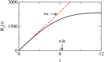
Figure 2: (color online) The second order decay rate $R_{2}(t)$ for the excitation current in the modular quantum system (black, solid curve). Parameters: $n=100$ and $\delta\epsilon=0.5$. This decay rate is well described by the linear approximation $4\,n\,t$ at a time scale below $\pi/\delta\epsilon$ (red, dashed line).

In the so far unexplored case of strong couplings the approach in Sec. III becomes applicable. The application only requires that the decay due to $\Delta\,V$ proceeds much faster than the decay due to $H_{0}$, i.e., $C(t)$ has to decay at a time scale $\tau<\tau_{0}$. If $\Delta$ is large, this requirement is naturally fulfilled. In fact, at such a time scale below $\tau_{0}$ no correlation function w.r.t. $H_{0}$ has decayed yet. Hence, the second order rate in Eq. (14) can be well described by the linear approximation in Eq. (17), see Fig. 2. The use of $\langle\imath[J,V]^{2}\rangle=8\,\Delta^{2}\,n^{2}$ and $\langle J^{2}\rangle=2\,\Delta^{2}\,n$ concretely leads to $r_{2}=4\,n$. The resulting second order prediction for the diffusion constant in Eq. (19) consequently is

$${\cal D}_{\text{strong}}(t)=\frac{1}{\Delta}\,\sqrt{\frac{\pi}{8\,n}}\,\frac{\langle J^{2}\rangle}{\langle X^{2}\rangle}=\sqrt{\frac{\pi\,n}{2}}\,\Delta=\text{const.}$$ (24)

above the relaxation time $\tau=1/(\sqrt{2\,n}\,\Delta)$. In Fig. 3 the analytical second order prediction is compared with the direct numerical result for the diffusion coefficient by the use of ED. Since for the modular quantum system the linear growth of the Hilbert space can be compensated by the translation symmetry, rather many modules are treatable. Apparently, the agreement between the second order prediction and numerics is very good, despite the limit of strong interactions. The minor deviations can be further reduced by fourth order corrections in terms of the cubic approximation in Eq. (18). Concretely, the use of $\langle[[J,V],V]^{2}\rangle=80\,\Delta^{2}\,n^{3}$ leads to $r_{4}=8\,n^{2}$. With such fourth order corrections the agreement in Fig. 3 becomes excellent. Remarkably, the corrections are small, because the ratio in Eq. (20) takes on the value $1/6$.

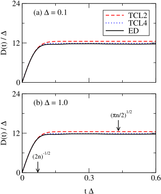
Figure 3: (color online) The time-dependent diffusion constant ${\cal D}(t)$ for the modular quantum system with strong interactions (a) $\Delta=0.1$, (b) $\Delta=1.0$. Parameters: $N=1000$, $n=100$, and $\delta\epsilon=0.5$. The theoretical predictions according to TCL2 (dashed, red curves) are already in good agreement with the numerical results from ED (solid, black curves), while minor corrections are given by the approximation of TCL4 (dotted, blue curves). As predicted by theory, ${\cal D}(t)$ takes on a constant value ${\cal D}\propto\Delta$ at intermediate times above the relaxation time $\tau\propto 1/\Delta$.

V Heisenberg Chain

In this Section spin transport in the Heisenberg spin chain will be investigated, as another concrete example for an interacting many-particle quantum system, going beyond the simplified single-particle model in the last Section. This investigation will firstly focus on a certain generalization of the standard Heisenberg spin-$1/2$ chain, taking into account the effect of anisotropic nearest and next-to-nearest neighbor interactions. The Hamiltonian concretely reads $H=H_{0}+\Delta V$, where the operators $H_{0}$ and $V$ are given by

$$H_{0}=J_{\mathrm{ec}}\sum_{r}s_{r}^{x}s_{r+1}^{x}+s_{r}^{y}s_{r+1}^{y}\,,$$ (25)

$$V=J_{\mathrm{ec}}\sum_{r}s_{r}^{z}s_{r+1}^{z}+\frac{\Delta_{2}}{\Delta}\,s_{r}^{z}s_{r+2}^{z}\,.$$ (26)

Here, $J_{\mathrm{ec}}$ is the exchange coupling constant, $\Delta$ refers to the anisotropy parameter, the matrix $s_{r}^{i}$ represents the $i$th component of the spin-$1/2$ operator at site $r$, and the parameter $\Delta_{2}$ specifies the strength of an additional next-to-nearest neighbor $zz$-interaction. For $\Delta_{2}=0$ the Hamiltonian obviously reduces to the usual anisotropic Heisenberg spin-$1/2$ chain (XXZ model).
The transport of spin or magnetization corresponds to local density operators $x_{r}=s_{r}^{z}$. Their sum is $S^{z}$ and a globally conserved quantity. Therefore, according to the scheme in Sec. II, the associated current can be written in the well-known form (see, e.g., the reviews zotos2003, ; heidrichmeisner2007, )

$$J=J_{\mathrm{ec}}\sum_{r}s_{r}^{x}s_{r+1}^{y}-s_{r}^{y}s_{r+1}^{x}$$ (27)

and commutates with $H_{0}$. In particular, $\langle J^{2}\rangle=J_{\mathrm{ec}}^{2}N/8$ and $\langle X^{2}\rangle=N/4$, where the trace operation is performed over the full $2^{N}$-dimensional Hilbert space. In fact, the following investigation will not be restricted to a specific $M$-subspace of $S^{z}$. However, the dominant contribution to transport stems from the largest subspaces around $M=0$ (‘half filling’). The dynamics in these subspaces can be diffusive, while the dynamics in the subspaces with $|M|\gg 0$ (‘dilute filling’) is expected to be ballistic, see below.

Since the eigensystem of $H_{0}$ is indispensable for the application of the introduced approach in Sec. III, it is convenient to perform the Jordan-Wigner transformation onto spin-less fermionsjordan1928 firstly and an additional Fourier transformation afterwards. The operators $H_{0}$, $V$, and $J$ in Eqs. (25)–(27) can then be rewritten asmahan2000

$$\!H_{0}=J_{\mathrm{ec}}\sum_{k}\epsilon_{k}\,n_{k}\,,\,\epsilon_{k}=\cos(k)\,,$$

$$\!V=\frac{J_{\mathrm{ec}}}{N}\sum_{k,l,q}v_{q}\,a_{k+q}^{\dagger}a_{l-q}^{\dagger}a_{l}a_{k}\,,\,v_{q}=e^{\imath q}+\frac{\Delta_{2}}{\Delta}e^{\imath 2q}\,,$$

$$\!J=J_{\mathrm{ec}}\sum_{k}j_{k}\,n_{k}\,,\,j_{k}=\frac{\partial\epsilon_{k}}{\partial k}=-\sin(k)\,.$$ (28)

Here, $n_{k}=a_{k}^{\dagger}a_{k}$ denotes the particle number operator for a spin-less fermion with the momentum $k=2\pi i/N$ and is written as the product of respective creation and annihilation operators. In this picture, $H_{0}$ describes the dispersion $\epsilon_{k}$ of non-interacting particles, while $V$ is the interaction between two particles, located at nearest or next-to-nearest sites, and $J$ plays the role of a particle current. Since $H_{0}$ and $J$ are both diagonal, $J$ is strictly preserved in the absence of $V$ and also in the one-particle subspace. As a consequence a single particle propagates ballistically.
If additional next-to-nearest neighbor $xx$-/$yy$-terms are added to Eq. (25) [and hence to Eq. (27)], such a picture can not be established: $H_{0}$ does not become diagonal by the use of the Jordan-Wigner transformation and $J$ does not commute with $H_{0}$. But these facts do not imply that the approach as such becomes not applicable. $H_{0}$ can be diagonalized at least numerically and, for large $\Delta$, the commutation of $J$ with $H_{0}$ is not required in the strict sense. Obviously, the situation is similar to the modular quantum system in Sec. IV. However, it turns out that the decay of $J$ w.r.t. $H_{0}$ is comparatively fast. This fast decay restricts the applicability of the approach to very large $\Delta$, i.e., close to the less interesting Ising limit. Thus, a situation with next-to-nearest neighbor $xx$-/$yy$-terms will not be discussed further.
For operators of the form in Eq. (28) an exact analytical formula for the second order decay rate $R_{2}(t)$ in Eq. (14) can be derived. In fact, the derivation of such a formula only requires the concrete evaluation of the expectation value $\langle[n_{k},V]_{\text{I}}(t)\,[n_{l},V]\rangle$ in the interaction picture, i.e., w.r.t. $H_{0}$. Even though the concrete evaluation appears to be a straightforward task at the first view, it turns out to be a both subtle and lengthy calculation. Nevertheless, after such a calculation the latter expectation value can be finally given as

$$\frac{\langle\imath[n_{k},V]_{\text{I}}(t)\,\imath[n_{l},V]\rangle}{\langle J^{2}\rangle}=\frac{2}{N^{3}}\sum_{q}$$

$$\!\!\delta_{k,l}\sum_{m}(\tilde{v}_{k-q}-\tilde{v}_{m-q})^{2}\cos[(\epsilon_{k}+\epsilon_{m}-\epsilon_{k+m-q}-\epsilon_{q})\,t]$$

$$\!\!+(\tilde{v}_{k-q}-\tilde{v}_{l-q})^{2}\cos[(\epsilon_{k}+\epsilon_{l}-\epsilon_{k+l-q}-\epsilon_{q})\,t]$$

$$\!\!-2\,(\tilde{v}_{k-q}-\tilde{v}_{l-k})^{2}\cos[(\epsilon_{q}+\epsilon_{l}-\epsilon_{q+l-k}-\epsilon_{k})\,t]$$ (29)

with $\tilde{v}_{k}=\text{Re}\,v_{k}$. Consequently, for a linear combination of the form $A_{i}=\sum_{k}a_{k}^{i}\,n_{k}$ one finds

$$R_{2}^{i,j}(t)\!\! = \!\!\int_{0}^{t}\!\text{d}t_{1}\,\frac{\langle\imath[A_{i},V]_{\text{I}}(t_{1})\,\imath[A_{j},V]\rangle}{\langle J^{2}\rangle}$$ (30)

$$= \!\!\frac{2}{N^{3}}\sum_{k,l,q}(a_{k}^{i}a_{k}^{j}+a_{k}^{i}a_{l}^{j}-2\,a_{q}^{i}a_{l}^{j})\,(\tilde{v}_{k-q}-\tilde{v}_{l-q})^{2}$$

$$\cdot \!\!\int_{0}^{t}\!\text{d}t_{1}\,\cos[(\epsilon_{k}+\epsilon_{l}-\epsilon_{k+l-q}-\epsilon_{q})\,t_{1}]\,,$$

including the second order decay rate $R_{2}(t)$ for $i=j=1$ and $a_{k}^{1}=j_{k}$. The more general notation in Eq. (30) will become useful later. Because this equation only involves a sum over three momenta $k$,$l$, and $q$, it can be evaluated numerically for several thousands of spins and, say, in the thermodynamic limit. Concretely, $N=2000$ will be chosen in the following. For that choice finite size effects do not appear at time scales up to $500/J_{\mathrm{ec}}$. For instance, such finite size effects occur at time scales on the order of $10/J_{\mathrm{ec}}$, if $N=20$ is chosen steinigeweg2010-2 , e.g., the maximum number of spins for ED.

V.1 The case $\Delta_{2}=\Delta$

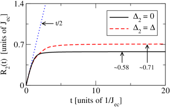
Figure 4: (color online) The second order decay rate $R_{2}(t)$ for the spin current in the anisotropic Heisenberg chain without additional terms (black, solid curve) and with an additional next-to-nearest neighbor $zz$-interaction of the same strength $\Delta_{2}=\Delta$ (red, dashed curve). Parameters: $N=2000$ [possible due to Eq. (30)]. These decay rates are well described by the linear approximation $t/2$ at a time scale below $1/J_{\mathrm{ec}}$ (blue, dotted line). Finite size effects do not occur at time scales up to $500/J_{\mathrm{ec}}$.

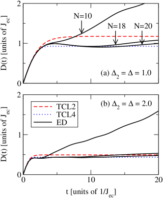
Figure 5: (color online) The time-dependent diffusion constant ${\cal D}(t)$ for spin transport in the anisotropic Heisenberg chain with an additional next-to-nearest neighbor $zz$-interaction of the same strength $\Delta_{2}=\Delta$ for large anisotropy parameter (a) $\Delta=1.0$ and (b) $\Delta=2.0$. The theoretical predictions of TCL2 for $N=2000$ (red, dashed curves) are already in good agreement with the numerical results from ED for $N=10$, $18$, and $20$ (black, solid curves). Additional corrections on the order of $20\%$ are given by the approximation of TCL4 (blue, dotted curves). In (a) the approximation of TCL4 is a slight overestimation.

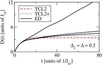
Figure 6: (color online) The time-dependent diffusion constant ${\cal D}(t)$ for spin transport in the anisotropic Heisenberg chain with an additional next-to-nearest neighbor $zz$-interaction of the same strength $\Delta_{2}=\Delta=0.5$. The theoretical prediction of TCL2 for $N=2000$ (red, dashed curve) is consistent with the numerical results from ED for $N=10$, $18$, and $20$ (black, solid curves). Another projection with more observables leads to a modified prediction TCL2+ for $N=200$ close to TCL2 (blue, dotted curve).

First, the case of additional next-to-nearest neighbor $zz$-interactions of the same strength may be discussed in detail, i.e., $\Delta_{2}=\Delta$. This particular case appears to be less controversial, since Drude weights are commonly expected to vanish in the thermodynamic limit due to non-integrability zotos1996 ; narozhny1998 ; rabson2004 , at least if $\Delta_{2}$ ($=\Delta$) does not become too small. For the case $\Delta_{2}=\Delta$ the second order decay rate $R_{2}(t)$ in Fig. 4 indeed takes on a form, as already considered in Sec. III: $R_{2}(t)$ firstly increases linearly at short time scales below $1/J_{\mathrm{ec}}$ and then becomes constant at longer time scales. Thus, the second order predictions for the diffusion coefficient $\cal D$ can directly be formulated according to Eqs. (16) and (19). By the use of $R_{2}\approx 0.71\,J_{\mathrm{ec}}$ from Fig. 4 and $r_{2}=1/2\,J_{\mathrm{ec}}^{2}$ these predictions read

$${\cal D}_{\text{weak}}\approx\frac{J_{\mathrm{ec}}}{\Delta^{2}}\,0.70\,,\,{\cal D}_{\text{strong}}=\frac{J_{\mathrm{ec}}}{\Delta}\,\frac{\sqrt{\pi}}{2}\,.$$ (31)

For anisotropy parameters above $\Delta\sim 1$ the decay of the current autocorrelation function takes place at a short time scale, i.e., where $R_{2}(t)$ scales more or less linearly with time. Since Drude weights for such $\Delta$ are already sufficiently small for $N\sim 20$, a direct comparison with the numerical results from ED becomes possible here, as shown in Fig. 5. By the use of the exact $R_{2}(t)$ in Fig. 4 the second order predictions for ${\cal D}(t)$ are already in good agreement with ED. Additional corrections on the order of $20\%$ are given by the fourth order approximation in Eq. (18). For $\Delta=1$ the latter approximation for short times seems to be a slight overestimation and may not be used further for smaller $\Delta$, i.e., when the relevant time scales for the decay of the current autocorrelation function become longer.
Since Drude weights always become dominant for small $\Delta$ and finite systems, a direct comparison between the second order prediction and the numerical results from ED is difficult in that case. But for $\Delta=0.5$ theory and numerics are at least consistent, see Fig. 6. Because the fourth order approximation is not available, the validity of the second order prediction may be confirmed by its independence from the chosen projection. To this end the projection may be extended to the full diagonal space, consisting of linear combinations $A_{i}$ of particle number operators $n_{k}$. As outlined in Sec. III, such a extension of the projection yields a rate matrix equation, namely,

$$\frac{\text{d}}{\text{d}t}\,\langle J(t)\,A_{i}\rangle=-\Delta^{2}\sum_{j}R_{2}^{i,j}(t)\,\langle J(t)\,A_{j}\rangle$$ (32)

with decay rates $R_{2}^{i,j}(t)$ according to Eq. (30). This rate matrix equation can be solved numerically by standard algorithms for, e.g., $N=200$. This modified prediction of, say, TCL2+ for $\Delta=0.5$ turns out to be rather close to the original prediction of TCL2, see Fig. 6. Because both predictions become identical for larger $\Delta$, TCL2+ is not indicated explicitly in Fig. 5. However, TCL2 and TCL2+ begin to differ significantly for smaller $\Delta$ and the validity of Eq. (31) in the limit of very weak interactions is questionable without the consideration of higher order decay rates.

V.2 The case $\Delta_{2}=0$

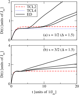
Figure 7: (color online) The time-dependent diffusion constant ${\cal D}(t)$ for spin transport in the anisotropic Heisenberg chain for the anisotropy $\Delta=1.5$ and the spin quantum numbers (a) $s=1/2$ and (b) $s=3/2$. The numerical results from ED (black, solid curves) are shown for (a) $N=10,18,20$ and (b) $N=7,8,9$. The TCL2 predictions (red, dashed curves) are based on the data in Fig. 4 and Ref. steinigeweg2010-2, , respectively. No TCL4 corrections (blue, dotted curve) are required in (b).

The case $\Delta_{2}=0$ is rather controversial due to the integrability of the Hamiltonian in terms of the Bethe Ansatz bethe1931 . In particular, for the isotropic point $\Delta=1$, there still is an unsettled debate about the finiteness of Drude weights in the thermodynamic limit: While Drude weights are widely expected to vanish for $\Delta>1$ heidrichmeisner2003 ; prelovsek2004 , they may already become zero for $\Delta=1$ zotos1999 ; benz2005 ; grossjohann2010 but definitely non-zero for all $0<\Delta<1$ prosen2011 , see also Ref. sirker2009, . However, in the present approach the situation is found to be similar to the previous case $\Delta_{2}=\Delta$, see Fig. 4. The second order decay rate $R_{2}(t)$ is almost the same, i.e., with a slightly reduced value $R_{2}\approx 0.58\,J_{\mathrm{ec}}$. Remarkably, the latter value can already be supposed on the basis of $N\sim 20$, i.e., $H_{0}$ in Eq. (28) contains only $10$ different energies steinigeweg2010-2 . Due to Fig. 4, the second order prediction for ${\cal D}_{\text{strong}}$ in Eq. (31) remains unchanged and ${\cal D}_{\text{weak}}$ becomes

$${\cal D}_{\text{weak}}\approx\frac{J_{\mathrm{ec}}}{\Delta^{2}}\,0.86\,.$$ (33)

But this prediction has to be considered carefully, since it depends on the chosen projection in the limit of very weak interactions, analogously to the case $\Delta_{2}=\Delta$. In fact, significant differences between TCL2 and TCL2+ occur already for $\Delta\sim 1$. Nevertheless, for larger $\Delta$ the TCL2 prediction is again found to be in good agreement with the numerical results from ED, see Fig. 7 (a). The additional incorporation of the TCL4 approximation in Eq. (18) goes beyond Ref. steinigeweg2010-2, and explains the reported deviations from ED and other approaches prelovsek2004 ; michel2008 ; prosen2009 , see also the perturbative approach in Ref. znidaric2011, .

V.3 The case $s>1/2$ ($\Delta_{2}=0$)

For spin quantum numbers $s>1/2$ the operators $H_{0}$, $V$, and $J$ in Eqs. (25)–(27) are formally identical. But in that case $H_{0}$ can not be brought into diagonal form by the use of the Jordan-Wigner transformation. The latter lack of a diagonal form is not a substantial drawback, since $J$ does not commutate with $H_{0}$ for $s>1/2$. Thus, the investigation is anyway restricted to the limit of strong interactions, similarly to the modular quantum system in Sec. IV. Such an investigation has already been done in detail in Ref. steinigeweg2010-2, . For illustration, however, an example for $s=3/2$ and $\Delta=1.5$ is shown in Fig. 7 (b). In a sense it is intriguing to see that the agreement between the theoretical prediction of TCL2 and the numerical result from ED is best, if $[J,H_{0}]\neq 0$, see also Fig. 3. It is worth to mention that the investigation in Ref. steinigeweg2010-2, suggests that, at high temperatures, the diffusion constant scales with the spin quantum number as ${\cal D}_{\text{strong}}\propto\sqrt{s(s+1)}$, see also Refs. huber1969-1, ; huber1969-2, ; karadamoglou2004, . This scaling supports classical simulations at high temperatures mueller1988 ; gerling1989 .

V.4 Alternating magnetic field ($\Delta_{2}=0$)

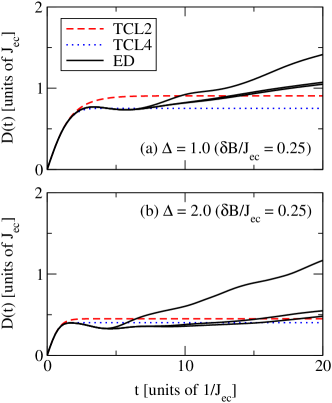
Figure 8: (color online) The time-dependent diffusion constant ${\cal D}(t)$ for spin transport in the anisotropic Heisenberg chain in the presence of an alternating magnetic field $\delta B/J_{\mathrm{ec}}=0.25$ for (a) $\Delta=1.0$ and (b) $\Delta=2.0$. The numerical results from ED (black, solid curves) are shown for $N=10$, $16$, and $18$. The theoretical predictions of TCL2 (red, dashed curves) are also based on numerical data for $N=18$, even though TCL2 does not depend on $N$ any further.

So far, the investigation at high temperatures does not depend on the presence of a homogenous magnetic field $B$ in $z$-direction, i.e., it does not change for an additional Zeeman term $H_{B}=BS^{z}$ in Eqs. (25) and (26). But the situation changes in the presence of an inhomogeneous magnetic field avishai2002 ; santos2004 ; santos2008 ; karahalios2009 , e.g., for an alternating sequence michel2008 ; prosen2009 ; steinigeweg2009-2 ; prosen2010

$$H_{B}=\sum_{r}\,\frac{B+(-1)^{r}\,\delta B}{\Delta}\,s_{r}^{z}\,,$$ (34)

where $\delta B$ denotes the strength of the alternation. Since $[J,H_{B}]\neq 0$, a magnetic field of this form represents an additional scattering mechanism and has to be added to $V$ in Eq. (26). In principle the alternating magnetic field in Eq. (34) may also be written in the representation of spin-less fermions and an exact analytical formula for the second order decay rate $R_{2}(t)$ may again be derived. But, because Eq. (34) obviously is no two-particle interaction, $R_{2}(t)$ is not of the form in Eq. (30). However, the case of an alternating magnetic field is primarily considered here in order to demonstrate potential difficulties of the approach at hand. For that reason the decay rate $R_{2}(t)$ is directly evaluated numerically for $N\sim 18$ by the use of ED jung2006 ; jung2007 , e.g., finite systems of this size are sufficient for the limit of strong interactions steinigeweg2010-2 . In Fig. 8 the resulting TCL2 prediction for ${\cal D}(t)$ is shown for $\delta B/J_{\mathrm{ec}}$ = 0.25 and different $\Delta$. Apparently, there still is a good agreement with the numerical results from ED apart from the, say, oscillation in Fig. 8 (b). This oscillation takes place after a zero-crossing of the underlying current autocorrelation function comment and is therefore not captured by the present approach. Because the amplitude of such oscillations is known to increase with the strength of the alternation steinigeweg2009-2 , the TCL2 approach yields only meaningful predictions for not too large $\delta B$.

VI Ising Chain

This Section will deal with another concrete quantum system which also allows to clarify potential difficulties of the approach at hand. This quantum system is an Ising spin-$1/2$ chain in the presence of a, say, tilted magnetic field. The Hamiltonian concretely reads $H=H_{0}+B_{z}\,V$, where the operators $H_{0}$ and V are given by mejiamonasterio2005 ; mejiamonasterio2007 ; prosen2009 ; steinigeweg2009-2

$$H_{0}=B_{x}\,S^{x}+J_{\mathrm{ec}}\sum_{r}s_{r}^{z}s_{r+1}^{z}\,,\,V=S^{z}\,,$$ (35)

where $B_{i}$ and $S^{i}$ are the $i$th component of the magnetic field ${\bf B}$ and total spin ${\bf S}$, respectively. For instance, one might think of a magnetic field which was originally in line with the $z$-direction and has been rotated about the $y$-axis with the angle $\alpha=\arctan(B_{x}/B_{z})$.
Since $[S^{z},H]\neq 0$ for this model, spin or magnetization is not a suitable transport quantity here. However, energy is always an appropriate transport quantity and may be investigated instead. In that case the corresponding local density operators read

$$x_{r}=\frac{B_{x}}{2}(s_{r}^{x}+s_{r+1}^{x})+J_{\mathrm{ec}}\,s_{r}^{z}s_{r+1}^{z}+\frac{B_{z}}{2}(s_{r}^{z}+s_{r+1}^{z})\,.$$ (36)

Thus, according to the scheme in Sec. II, the associated current is given by

$$J=\frac{J_{\mathrm{ec}}\,B_{x}}{2}\sum_{r}(s_{r+2}^{z}-s_{r}^{z})\,s_{r+1}^{y}$$ (37)

and $[J,H_{0}]=0$. Particularly, $\langle J^{2}\rangle=NJ_{\mathrm{ec}}^{2}B_{x}^{2}/32$ as well as $\langle X^{2}\rangle=N(4B_{x}^{2}+J_{\mathrm{ec}}^{2}+4B_{z}^{2})/16$.

Because of the commutation of the operators $J$ and $H_{0}$ a second order prediction may be formulated for the limit of weak ‘interactions’, i.e., small $z$-components of the magnetic field. In fact, direct numerics for $N\sim 16$ by the use of ED already indicate a well-behaved second order decay rate $R_{2}(t)$, i.e., $R_{2}(t)$ appears to take on a constant value at long time scales, see Fig. 9. Although $N\sim 16$ is still far away from the thermodynamic limit, the convergence with $N$ in Fig. 9 seems to be at least rather indicative for a constant value. However, since at short time scales $R_{2}(t)$ shows a non-trivial dependence on time, such a dependence certainly occurs also for higher order decay rates. In particular higher order decay rates may not develop towards constant values at long time scales. On that account a second order prediction has to be considered carefully here, see Sec. III.
Nevertheless, the convergence in Fig. 9 is sufficient for strong interactions steinigeweg2010-2 , analogously to the previous case of an alternating magnetic field. The resulting second order prediction for ${\cal D}(t)$ is shown in Fig. 10 for equally large components of the magnetic field, i.e., $B_{x}/B_{z}\sim 1$. The use of the fourth order approximation again allows to correctly describe ${\cal D}(t)$ up to the (first) zero-crossing of the underlying current autocorrelation function comment . But, in contrast to the decrease in Fig. 8, a renewed increase of ${\cal D}(t)$ emerges after this zero-crossing, resulting from partial revivals of the current autocorrelation function, e.g., due to a spectrum which gradually becomes closer to the equidistant levels of the pure Ising model (with a magnetic field in $z$-direction). This renewed increase of ${\cal D}(t)$ remarkably turns out to be captured by the mere second order prediction. Therefore the present example clearly illustrates that fourth order corrections improve usually the description at short time scales but do not yield necessarily to a better description at larger time scales, e.g., after a potential zero-crossing of the current autocorrelation function.

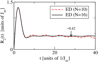
Figure 9: (color online) The second order decay rate $R_{2}(t)$ for the energy current in the Ising chain in the presence of a tilted magnetic field for $N=10$ and $16$. Parameters: $B_{x}/J_{\mathrm{ec}}=0.85$.

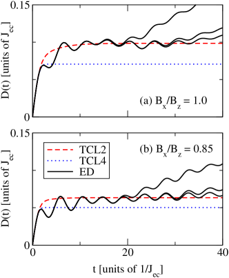
Figure 10: (color online) The time-dependent diffusion constant ${\cal D}(t)$ for energy transport in the Ising chain in the presence of a tilted magnetic field for (a) $B_{x}/B_{z}=1.0$ ($\alpha=45^{\circ}$) and (b) $B_{x}/B_{z}=0.85$ ($\alpha\approx 40^{\circ}$). Parameters: $B_{x}/J_{\mathrm{ec}}=0.85$. The numerical results from ED (black, solid curves) are shown for $N=10$, $14$, and $16$. The theoretical predictions according to TCL2 (red, dashed curves) are also based on numerical data for $N=16$ in Fig. 9.

VII Summary and Conclusion

The present paper has studied the decay of current autocorrelation functions for quantum systems featuring strong ‘interactions’. In this study the term interaction has referred to that part of the Hamiltonian causing the (major) decay of the current. To this end an appropriate perturbation theory in the interaction strength has been introduced at first, namely, by an application of the TCL projection operator technique. For the addressed case of strong interactions the quality of a truncation to lowest order has been demonstrated to depend on the form of the interaction and not on its strength as such. By the use of the introduced perturbation theory the diffusion coefficient has been evaluated afterwards for a variety of transport quantities in concrete quantum systems. This evaluation has been started for excitation transport in the modular quantum system and has been continued for spin and energy transport in several spin chains. For all examples the lowest order prediction for the diffusion constant has well agreed with the numerical results from ED, even in the case of strong interactions. Remarkably, higher order corrections have played a minor role.

The investigation has focused on high temperatures and one-dimensional quantum systems so far. Both have been chosen here in order to allow for a comparison with the numerical results from ED, being more or less free of finite size effects for this particular choice. However, the introduced perturbation theory is not restricted to one dimension. But this perturbation theory probably is restricted to high temperatures, at least in the addressed case of strong interactions. Low temperatures confine the perturbation theory in the form at hand to the case of weak interactions: Only for that case an approximation of the statistical operator on the basis of the uncoupled system is expected to be reliable at all. Nevertheless, in the context of weak interactions, higher order corrections probably play a more important role, similarly to high temperatures. In any case further estimations for higher order contributions certainly are desirable, not only for the projection onto currents but also for the alternative projection onto densities. These projections have already been applied successfully for one-particle models steinigeweg2007 ; steinigeweg2010-1 .

- (1) R. Kubo, M. Yokota, and S. Hashtisume, Statistical Physics II: Nonequilibrium Statistical Mechanics, 2nd ed., Solid State Sciences (Springer, New York, 1991)
- (2) G. D. Mahan, Many Particle Physics, 3rd ed., Physics of Solids and Liquids (Springer, New York, 2000)
- (3) J. Sirker, R. G. Pereira, and I. Affleck, Phys. Rev. Lett. 103, 216602 (2009)
- (4) S. Nakajima, Progr. Theor. Phys. 20, 948 (1958)
- (5) R. Zwanzig, J. Chem. Phys. 33, 1338 (1960)
- (6) H. Mori, Progr. Theor. Phys. 33, 423 (1965)
- (7) D. Forster, Hydrodynamic Fluctuations, Broken Symmetry, and Correlation Functions (Benjamin, Massachusetts, 1975)
- (8) S. Chaturvedi and F. Shibata, Z. Phys. B 35, 297 (1979)
- (9) H.-P. Breuer and F. Petruccione, The Theory of Open Quantum Systems (Oxford University Press, New York, 2007)
- (10) C. Mejía-Monasterio and H. Wichterich, Eur. Phys. J. Spec. Top. 151, 113 (2007)
- (11) M. Michel, O. Hess, H. Wichterich, and J. Gemmer, Phys. Rev. B 77, 104303 (2008)
- (12) T. Prosen and M. Žnidarič, J. Stat. Mech. 2009, P02035 (2009)
- (13) R. Steinigeweg, M. Ogiewa, and J. Gemmer, EPL 87, 10002 (2009)
- (14) T. Prosen and M. Žnidarič, Phys. Rev. Lett. 105, 060603 (2010)
- (15) T. Prosen, Phys. Rev. Lett. 106, 217206 (2011)
- (16) M. Žnidarič, Phys. Rev. Lett. 106, 220601 (2011)
- (17) P. Jung, R. W. Helmes, and A. Rosch, Phys. Rev. Lett. 96, 067202 (2006)
- (18) P. Jung and A. Rosch, Phys. Rev. B 76, 245108 (2007)
- (19) R. Steinigeweg and R. Schnalle, Phys. Rev. E 82, 040103(R) (2010)
- (20) R. Steinigeweg, H.-P. Breuer, and J. Gemmer, Phys. Rev. Lett. 99, 150601 (2007)
- (21) X. Zotos and P. Prelov̌sek, Interacting Electrons in Low Dimensions, Physics and Chemistry of Materials with Low-Dimensional Structures (Kluwer Academic, Dordrecht, 2004)
- (22) F. Heidrich-Meisner, A. Honecker, and W. Brenig, Eur. Phys. J. Spec. Top. 151, 135 (2007)
- (23) P. Prelovšek, S. El Shawish, X. Zotos, and M. Long, Phys. Rev. B 70, 205129 (2004)
- (24) D. L. Huber and J. S. Semura, Phys. Rev. 182, 602 (1969)
- (25) D. L. Huber, J. S. Semura, and C. G. Windsor, Phys. Rev. 186, 534 (1969)
- (26) J. Karadamoglou and X. Zotos, Phys. Rev. Lett. 93, 177203 (2004)
- (27) R. Steinigeweg, H. Wichterich, and J. Gemmer, EPL 88, 10004 (2009)
- (28) S. Goldstein, J. L. Lebowitz, R. Tumulka, and N. Zanghi, Phys. Rev. Lett. 96, 050403 (2006)
- (29) S. Popescu, A. J. Short, and A. Winter, Nature Phys. 2, 754 (2006)
- (30) P. Reimann, Phys. Rev. Lett. 99, 160404 (2007)
- (31) C. Bartsch and J. Gemmer, Phys. Rev. Lett. 102, 110403 (2009)
- (32) R. Steinigeweg and J. Gemmer, Phys. Rev. B 80, 184402 (2009)
- (33) J. Gemmer, R. Steinigeweg, and M. Michel, Phys. Rev. B 73, 104302 (2006)
- (34) P. W. Anderson, Phys. Rev. 109, 1492 (1958)
- (35) R. Steinigeweg, H. Niemeyer, and J. Gemmer, New J. Phys. 12, 113001 (2010)
- (36) P. Jordan and E. Wigner, Z. Phys. 47, 631 (1928)
- (37) X. Zotos and P. Prelovšek, Phys. Rev. B 53, 983 (1996)
- (38) B. N. Narozhny, A. J. Millis, and N. Andrei, Phys. Rev. B 58, 2921(R) (1998)
- (39) D. A. Rabson, B. N. Narozhny, and A. J. Millis, Phys. Rev. B 69, 054403 (2004)
- (40) H. Bethe, Z. Phys. A 71, 205 (1931)
- (41) F. Heidrich-Meisner, A. Honecker, D. C. Cabra, and W. Brenig, Phys. Rev. B 68, 134436 (2003)
- (42) X. Zotos, Phys. Rev. Lett. 82, 1764 (1999)
- (43) J. Benz, T. Fukui, A. Klümper, and C. Scheeren, J. Phys. Soc. Jpn. 74, 181 (2005)
- (44) S. Grossjohann and W. Brenig, Phys. Rev. B 81, 012404 (2010)
- (45) G. Müller, Phys. Rev. Lett. 60, 2785 (1988)
- (46) R. W. Gerling and D. P. Landau, Phys. Rev. Lett. 63, 812 (1989)
- (47) Y. Avishai, J. Richert, and R. Berkovits, Phys. Rev. B 66, 052416 (2002)
- (48) L. F. Santos, J. Phys. A 37, 4723 (2004)
- (49) L. F. Santos, Phys. Rev. E 78, 031125 (2008)
- (50) A. Karahalios, A. Metavitsiadis, X. Zotos, A. Gorczyca, and P. Prelovšek, Phys. Rev. B 79, 024425 (2009)
- (51) Since , a local extremum of implies a zero-crossing of .
- (52) C. Mejía-Monasterio, T. Prosen, and G. Casati, Europhys. Lett. 72, 520 (2005)