Analysis of Equilibria and Strategic Interaction in Complex Networks

Abstract

This paper studies $n$-person simultaneous-move games with linear best response function, where individuals interact within a given network structure. This class of games have been used to model various settings, such as, public goods, belief formation, peer effects, and oligopoly. The purpose of this paper is to study the effect of the network structure on Nash equilibrium outcomes of this class of games. Bramoullé et al. derived conditions for uniqueness and stability of a Nash equilibrium in terms of the smallest eigenvalue of the adjacency matrix representing the network of interactions. Motivated by this result, we study how local structural properties of the network of interactions affect this eigenvalue, influencing game equilibria. In particular, we use algebraic graph theory and convex optimization to derive new bounds on the smallest eigenvalue in terms of the distribution of degrees, cycles, and other relevant substructures. We illustrate our results with numerical simulations involving online social networks.

I Introduction

In most social and economic settings, individuals do not interact uniformly with the rest of a society. Instead, they influence each other according to a structured network of interactions. This network can represent friendships in a social network, transactions among firms in a market, or communication links in a process of belief formation. In this context, an interesting question is to study how the network structure affects the outcome of the interactions of the agents. With this purpose, one can model strategic interactions in a networked society as a multi-player simultaneous-move game. In particular, we focus our attention on the broad class of games with linear best response function [1]. This class of games have been used to model various settings such as belief formation [2], peer effects [3], and public goods [4].

In order to analyze the influence of the network structure on the game outcome, we use two recent results by Bramoullé et al. [5] and Ballester et al. [6] relating the Nash equilibria of the game with the largest and smallest eigenvalues of the adjacency matrix of interactions. For example, in [5], the authors show that uniqueness and stability of a Nash equilibrium in games with linear best responses can be determined by the smallest eigenvalue of the network. In [5], it was also illustrated how the smallest eigenvalue of the adjacency matrix determines the capacity of the network to absorb perturbations on the actions of the agents.

Motivated by the results of Bramoullé et al. [5], we study how local structural properties of the network affect the smallest eigenvalue of the adjacency matrix of interactions, affecting game equilibria. Therefore, our results build a bridge between structural properties of a network of interactions and the outcome of games with linear best responses. In particular, we use algebraic graph theory and convex optimization to derive bounds on the smallest eigenvalue of the adjacency matrix in terms of the distribution of degrees, cycles, and other important substructures. As we illustrate with numerical simulations in online social networks, these bounds can be used to estimate the effect of structural perturbations on the smallest eigenvalue.

The paper is organized as follows. In the next subsection, we review graph-theoretical terminology needed in our derivations. In Section II, we review the relationship between the equilibria of games with linear best responses in a network and the smallest eigenvalue of the adjacency matrix of interactions. In Section III, we use algebraic graph theory to derive closed-form expressions for the so-called spectral moments of a network in terms of local structural features. In Section IV, we use convex optimization to derive optimal bounds on the smallest (and largest) eigenvalue of the interaction network from these moments. Our bounds help us to understand how structural properties of a network impact the stability properties of the Nash equilibria in the game. We illustrate our results with numerical simulations in real online social networks in Section V.

I-A Notation

Let $\mathcal{G}=\left(\mathcal{V},\mathcal{E}\right)$ denote an undirected graph with $n$ nodes, $e$ edges, and no self-loops. We denote by $\mathcal{V}\left(\mathcal{G}\right)=\left\{v_{1},\dots,v_{n}\right\}$ the set of nodes and by $\mathcal{E}\left(\mathcal{G}\right)\subseteq\mathcal{V}\left(\mathcal{G}\right)\times\mathcal{V}\left(\mathcal{G}\right)$ the set of undirected edges of $\mathcal{G}$. If $\left\{v_{i},v_{j}\right\}\in\mathcal{E}\left(\mathcal{G}\right)$ we call nodes $v_{i}$ and $v_{j}$ adjacent (or neighbors), which we denote by $v_{i}\sim v_{j}$ and define the set of neighbors of $v_{i}$ as $\mathcal{N}_{i}=\{w\in\mathcal{V}\left(\mathcal{G}\right):\left\{v_{i},w\right\}\in\mathcal{E}\left(\mathcal{G}\right)\}$. The number of neighbors of $v_{i}$ is called the degree of the node, denoted by $d_{i}$. We define a walk of length $k$ from $v_{0}$ to $v_{k}$ to be an ordered sequence of nodes $\left(v_{0},v_{1},...,v_{k}\right)$ such that $v_{i}\sim v_{i+1}$ for $i=0,1,...,k-1$. If $v_{0}=v_{k}$, then the walk is closed. A closed walk with no repeated nodes (with the exception of the first and last nodes) is called a cycle. For example, triangles, quadrangles and pentagons are cycles of length three, four, and five, respectively.

Graphs can be algebraically represented via matrices. The adjacency matrix of an undirected graph $\mathcal{G}$, denoted by $A_{\mathcal{G}}=[a_{ij}]$, is an $n\times n$ symmetric matrix defined entry-wise as $a_{ij}=1$ if nodes $v_{i}$ and $v_{j}$ are adjacent, and $a_{ij}=0$ otherwise. The eigenvalues of $A_{\mathcal{G}}$, denoted by $\lambda_{1}\geq\lambda_{2}\geq\ldots\geq\lambda_{n}$, play a key role in our paper. The spectral radius of $A_{\mathcal{G}}$, denoted by $\rho\left(A_{\mathcal{G}}\right)$, is the maximum among the magnitudes of its eigenvalues. Since $A_{\mathcal{G}}$ is a symmetric matrix with nonnegative entries, all its eigenvalues are real and the spectral radius is equal to the largest eigenvalue, $\lambda_{1}$. We define the $k$-th spectral moment of the adjacency matrix $A_{\mathcal{G}}$ as:

$$m_{k}\left(A_{\mathcal{G}}\right)=\frac{1}{n}\sum_{i=1}^{n}\lambda_{i}^{k}.$$ (1)

As we shall show in Section III, there is a direct connection between the spectral moments and the presence of certain substructures in the graph, such as cycles of length $k$.

II Strategic Interactions in Networks

In this section we present the game-theoretical model of strategic interactions considered in this paper and present interesting connections between the Nash equilibria and the eigenvalues of the adjacency matrix of the network.

II-A The Model

We represent the network of influences using a simple graph $\mathcal{G}$. Let $\mathcal{N}=\{1,\cdots,n\}$ denote the set of $n$ players located at each node of the graph $\mathcal{G}$. We denote by $x_{i}\in[0,\infty)$ the action chosen by agent $i$, and by $\mathbf{x}$ the vector that represents the joint actions for all agents. We denote by $\mathbf{x}_{-i}$ the vector of actions of all players excluding player $i$. As mentioned before, players interact according to a network of influences that we describe using its adjacency matrix $A_{\mathcal{G}}$. The interactions are assumed to be symmetric, $a_{ij}=a_{ji}$, and we do not allow self-loops, $a_{ii}=0$. The payoff function for agent $i$ is given by:

$$U_{i}(x_{i},\mathbf{x}_{-i};\delta,A_{\mathcal{G}})$$

where $\delta\in\mathbb{R}$ is a parameter that can be tuned to change the influence of neighboring nodes on each player’s action.

II-B Games with Linear Best Response Functions

We study a class of games whose best response functions take a linear form. One well known example of this class of games is the differentiated-product Cournot oligopoly with linear inverse demand and constant marginal cost with payoff function defined as [5]:

$$U_{i}(x_{i},\mathbf{x}_{-i};\delta,A_{\mathcal{G}})=x_{i}\left(a-b(x_{i}+2\delta\sum_{j=1}^{n}a_{ij}x_{j})\right)-dx_{i},$$ (2)

where $d$ is the constant marginal cost, and $x_{i}$ represents the amount produced by agent $i$ in the oligopoly. Here, the inverse demand for agent $i$ is given by $P_{i}(x_{i},\mathbf{x}_{-i};\delta,A_{\mathcal{G}})=a-b(x_{i}+2\delta\sum_{j=1}^{n}a_{ij}x_{j})$. One can prove that the best response function for this type of games yield the form [5]:

$$f_{i}(\mathbf{x},\delta,A_{\mathcal{G}})=\max(0,\bar{x}_{i}-\delta\sum_{j=1}^{n}a_{ij}x_{j}),$$ (3)

where $\bar{x}_{i}$ is the action that agent $i$ would take in isolation, i.e., $\bar{x}_{i}\in\arg\max_{x_{i}}U_{i}(x_{i},\mathbf{x}_{-i};\delta,A_{\mathcal{G}})$ with $a_{ij}=0$,  for all $j$. Without loss of generality, one can normalize $\bar{x}_{i}\equiv 1$ for all $i$, so that $f_{i}(\mathbf{x})\in[0,1]$. Then, a Nash equilibrium for this game is a vector $\mathbf{x}\in[0,1]^{n}$ that satisfies $x_{i}=f_{i}(\mathbf{x},\delta,A_{\mathcal{G}})$, for all agents $i\in\mathcal{N}$, simultaneously. In what follows, we briefly describe a strategy to compute the complete set of Nash equilibria for $\delta\in[0,1]$.

II-C Complete Set of Nash Equilibria

Using the best response function in (3), one can determine the entire set of equilibria by simultaneously solving for the best response of each player. In [5], an algorithm that finds the full set of Nash equilibria in exponential time is proposed. For a vector $\mathbf{x}$, let $S$ denote the set of active agents, i.e., $S=\{i:x_{i}>0\}$. Let $\mathbf{x}_{S}$ denote the vector of actions of the agents in $S$. The set of active players induce a subgraph $\mathcal{G}_{S}\subseteq\mathcal{G}$, with node-set $S\subseteq\mathcal{V}\left(\mathcal{G}\right)$ and a set of edges $\mathcal{E}_{S}\subseteq\mathcal{E}\left(\mathcal{G}\right)$ connecting active agents. We denote by $\mathcal{G}_{\mathcal{N}\backslash S,S}$ the subgraph of $\mathcal{G}$ whose edges connect active agents in $S$ to inactive agents in $\mathcal{N}\backslash S$. The adjacency matrices of $\mathcal{G}_{S}$ and $\mathcal{G}_{\mathcal{N}\backslash S,S}$ are denoted by $A_{S}\in\mathbb{R}^{\left|S\right|\times\left|S\right|}$ and $A_{\mathcal{N}\backslash S,S}\in\mathbb{R}^{n-\left|S\right|\times\left|S\right|}$, respectively. Then, one can show the following [5]:

Proposition 1

A profile $\mathbf{x}$ with active agents $S$ is a Nash equilibrium if and only if:

$$(I_{\left|S\right|}+\delta A_{S})\mathbf{x}_{S} = \mathbf{1}_{\left|S\right|}\mathbf{,}\text{ and}$$

$$\delta A_{\mathcal{N}\backslash S,S}~{}\mathbf{x}_{S} \geq \mathbf{1}_{n-\left|S\right|}\mathbf{,}$$

where $I_{p}$ is the $p\times p$ identity matrix and $\mathbf{1}_{q}$ is the $q$-dimensional vector of ones.

Thus, in order to determine the complete set of all Nash equilibria, one can check the conditions in Proposition 1 for each one of the $2^{n}$ possibilities of $S$. For each possible $S$, these conditions can be checked by computing $\mathbf{x}_{S}=(I_{\left|S\right|}+\delta A_{S})^{-1}\mathbf{1}_{\left|S\right|}$, and checking whether $\delta A_{\mathcal{N}\backslash S,S}~{}\mathbf{x}_{S}\geq\mathbf{1}_{n-\left|S\right|}$. If the last inequality holds, then $\mathbf{x}_{S}$ is an equilibrium outcome. Note that using this approach to compute the set of equilibria runs in exponential time. However, we can analyze some properties of the Nash equilibria, such as uniqueness and stability, by looking into the eigenvalues of the adjacency matrix.

II-D The Shape of Nash Equilibria

In order to relate the equilibrium outcomes of the game to the network structure, the authors in [5] defined the following potential function:

$$\varphi(\mathbf{x};\delta,A_{\mathcal{G}})\triangleq\sum_{i=1}^{n}\left(x_{i}-\frac{1}{2}x_{i}^{2}\right)-\frac{1}{2}\delta\sum_{i=1}^{n}\sum_{j=1}^{n}a_{ij}x_{i}x_{j}.$$

Then, they proved, using Kuhn-Tucker conditions, that the set of Nash equilibria coincides with the critical points of the following optimization problem:

$$\begin{array}[]{lll}(\text{P})&\max_{\mathbf{x}}&\varphi(\mathbf{x};\delta,A_{\mathcal{G}})\\ &s.t.&x_{i}\geq 0,\text{ for all }i,\end{array}$$

for a given network structure $A_{\mathcal{G}}$ and a parameter $\delta$.

II-E Eigenvalues and Nash Equilibria

We can find several results in the literature providing sufficient conditions for the existence of a unique Nash equilibrium in games with linear best response functions in terms of the eigenvalues of the network of influences. We enumerate below some sufficient conditions that are related with our work:

Proposition 2

Consider the class of games with linear best response functions described in Section II-B. For these games, we have the following sufficient conditions for the existence of a unique Nash equilibrium:

(i)

$\delta<-1/\lambda_{n}(A_{\mathcal{G}})$, (Bramoullé et al., [5]).

(ii)

$\delta<1/\rho\left(A_{\mathcal{G}}\right)$, (Ballester et al., [6]).

We can compare the set of spectral conditions in Proposition 2 using the following inequalities [5]:

Lemma 3

For any simple graph $\mathcal{G}$, we have that $-1/\lambda_{n}(A_{\mathcal{G}})\geq 1/\rho\left(A_{\mathcal{G}}\right)$, where this inequality is strict when no component of $\mathcal{G}$ is bipartite.

Remark 4

Hence, Condition (i) in Proposition 2 provides the best sufficient condition for the uniqueness of Nash equilibrium in these games. Furthermore, one can also prove that under Condition (i) or (ii), all players are active at the equilibrium point, i.e., $S=\mathcal{N}$ [5].

In Section IV, we shall derive upper bounds on $\lambda_{n}\left(A_{\mathcal{G}}\right)$ in terms of structural properties of the network. These bounds, in combination with Condition (i) in Proposition 2, will allow us to derive sufficient conditions for the existence of a Nash equilibrium in terms of structural properties of the network.

II-F The Stability of Nash Equilibria

We present conditions for stability of a Nash equilibrium in terms of $\lambda_{n}(A_{S})$. A Nash equilibrium $\mathbf{x}$ is asymptotically stable when the system of differential equations:

$$\begin{array}[]{c}\dot{x}_{1}=h_{1}(\mathbf{x})=f_{1}(\mathbf{x};\delta,A_{\mathcal{G}})-x_{1},\\ \vdots\\ \dot{x}_{n}=h_{n}(\mathbf{x})=f_{n}(\mathbf{x};\delta,A_{\mathcal{G}})-x_{n},\end{array}$$

is locally asymptotically stable around $\mathbf{x}$. One can prove the following necessary and sufficient condition for an equilibrium $\mathbf{x}$ to be asymptotically stable [5]:

Lemma 5

An equilibrium profile $\mathbf{x}$ is asymptotically stable if and only if $\delta<-1/\lambda_{n}(A_{S})$ and $\delta\sum_{j=1}^{n}a_{ij}x_{j}>1,$ for all inactive agents $i\in\mathcal{N}\backslash S$.

From the above lemma and Remark 4, we conclude that if $\delta<-1/\lambda_{n}(A_{\mathcal{G}})$, there is a unique Nash equilibrium and it is asymptotically stable. These results show the close connection between the smallest and the largest eigenvalues of the adjacency matrix of interactions and the outcome of games with linear best response functions in a network. On the other hand, the results in this section are applicable if we are able to compute the eigenvalues of $A_{\mathcal{G}}$. For many large-scale complex networks, the structure of the network can be very intricate [9]-[11] —in many cases not even known exactly— and an explicit eigenvalue decomposition can be very challenging to compute, if not impossible. In many practical settings, instead of having access to the complete network topology, we have access to local neighborhoods of the network structure around a set of nodes. In this context, it is important to understand the impact of local structural information on the eigenvalues of the adjacency matrix. In the rest of the paper, we propose a novel methodology to compute optimal bounds on relevant eigenvalues of $A_{\mathcal{G}}$ from local information regarding the network structure. Our results allow us to study the role of local structural information in the outcome of games with linear best response functions.

III Spectral Analysis of the Interaction Matrix

We study the relationship between a network’s local structural properties and the smallest eigenvalue of its adjacency matrix. Algebraic graph theory provides us with tools to relate the eigenvalues of a network with its structural properties. Particularly useful is the following well-known result relating the $k$-th spectral moment of $A_{\mathcal{G}}$ with the number of closed walks of length $k$ in $\mathcal{G}$ [7]:

Lemma 6

Let $\mathcal{G}$ be a simple graph. The $k$-th spectral moment of the adjacency matrix of $\mathcal{G}$ can be written as

$$m_{k}(A_{\mathcal{G}})=\frac{1}{n}\sum_{i=1}^{n}\lambda_{i}^{k}=\frac{1}{n}\left|\Psi_{\mathcal{G}}^{\left(k\right)}\right|,$$ (4)

where $\Psi_{\mathcal{G}}^{\left(k\right)}$ is the set of all closed walks of length $k$ in $\mathcal{G}$.

From (4), we can easily compute the first three spectral moments of $A_{\mathcal{G}}$ in terms of the number of nodes, edges and triangles as follows [7]:

Corollary 7

Let $\mathcal{G}$ be a simple graph with adjacency matrix $A_{\mathcal{G}}$. Denote by $n$, $e$ and $\Delta$ the number of nodes, edges and triangles in $\mathcal{G}$, respectively. Then,

$$m_{1}(A_{\mathcal{G}}) =0,$$ (5)

$$m_{2}(A_{\mathcal{G}}) =2e/n,$$

$$m_{3}(A_{\mathcal{G}}) =6\,\Delta/n.$$

Remark 8

Notice that the coefficients 2 (resp. 6) in the above expressions corresponds to the number of closed walks of length 2 (resp. 3) enabled by the presence of an edge (resp. triangle). Similar expressions can be derived for higher-order spectral moments, although a more elaborated combinatorial analysis in required.

In our case, we are interested in the following expressions, derived in [8], for the first five spectral moments of $\mathcal{G}$:

Lemma 9

Let $\mathcal{G}$ be a simple graph. Denote by $e$, $\Delta$, $Q$ and $\Pi$ the total number of edges, triangles, quadrangles and pentagons in $\mathcal{G}$, respectively. Define $W_{2}=\sum_{i=1}^{n}d_{i}^{2}$ and $\mathcal{C}_{dt}=\sum_{i}d_{i}t_{i}$, where $t_{i}$ is the number of triangles touching node $i$. Then,

$$m_{4}\left(A_{\mathcal{G}}\right) = \frac{1}{n}\left[8Q+2W_{2}-e\right],$$ (6)

$$m_{5}\left(A_{\mathcal{G}}\right) = \frac{1}{n}\left[10\Pi+10\mathcal{C}_{dt}-30\Delta\right].$$ (7)

Observe how, as we increase the order of the moments, more complicated structural features appear in the expressions. In the following example, we illustrate how to use our expressions to compute the spectral moments of an online social network from empirical structural data.

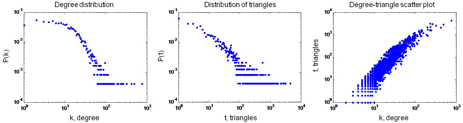
Figure 1: In the left and center figures, we plot the distributions of degrees and triangles of the social network under study (in log-log scale). In the right figure, we include a scatter plot where each point has coordinates $(d_{i},t_{i})$, in log-log scale, for all the nodes in the social graph.

Example 10

In this example, we study a subgraph of Facebook obtained by exploring the online social network around a particular node, as follows. From a particular starting node, we crawl the network (using a breadth-first search) until we discover the set of all nodes that are within a radius $2$ from the starting node. Using this set of nodes, and their interconnections (friendships), we construct a social subgraph $\mathcal{F}$ that has $2,404$ nodes and $22,786$ edges. Using this real dataset, we compute the degrees $d_{i}$, the number of triangles $t_{i}$, quadrangles $q_{i}$, and pentagons $p_{i}$ touching each node $i\in\mathcal{V}\left(\mathcal{F}\right)$. In Fig. 1, we plot the distributions of degrees and triangles, as well as a scatter plot of $t_{i}$ versus $d_{i}$ (where each point has coordinates $\left(d_{i},t_{i}\right)$, in log-log scale, for all $i\in\mathcal{V}\left(\mathcal{F}\right)$). We can aggregate those quantities that are relevant to compute the spectral moments to obtain the following numerical values:

$$\begin{array}[]{ll}e/n=\sum d_{i}/2n=9.478,&\Delta/n=\sum t_{i}/3n=28.15,\\ Q/n=\sum q_{i}/4n=825.3,&\Pi/n=\sum p_{i}/5n=31,794,\\ W_{2}/n=\sum d_{i}^{2}/n=1,318,&\mathcal{C}_{dt}/n=\sum d_{i}t_{i}/n=8,520.\end{array}$$

Hence, using Corollary 7 and Lemma 9, we obtain the following values for the spectral moments: $m_{1}\left(A_{\mathcal{F}}\right)=0,$ $m_{2}\left(A_{\mathcal{F}}\right)=18.95,$ $m_{3}\left(A_{\mathcal{F}}\right)=168.9,$ $m_{4}\left(A_{\mathcal{F}}\right)=9,230,$ and $m_{5}\left(A_{\mathcal{F}}\right)=402,310.$

In this section, we have derived expressions to compute the first five spectral moment of $A_{\mathcal{G}}$ from network structural properties. In the next section, we use semidefinite programming to extract information regarding eigenvalues of interest from a sequence of spectral moments.

IV Optimal Spectral Bounds from Spectral Moments

Here, we introduce an approach to derive an upper bound on the smallest eigenvalues of $A_{\mathcal{G}}$ from its sequence of spectral moments. Since we have expressions for the spectral moments in terms of local structural properties, our bounds relate the eigenvalues of a network with these properties. There is a large literature studying the relationship between structural and spectral properties of graphs (see [12],[13], and references therein, for an extensive list of spectral results). For many real-world networks, there is a particular set of structural properties that play a key role in the network’s functionality. For example, it is well-known that social networks contain a large number of triangles (and other cycles). Hence, it would be useful to have spectral bounds where these structural features are jointly represented. In this section, we derive new upper bounds on the smallest eigenvalue of the adjacency matrix in terms of the structural properties involved in (5), (6) and (7). Our results can be easily extended to derive lower bounds on the spectral radius of the adjacency matrix, although this bound is not of relevance in our analysis of games with linear best responses.

Now, we derive bounds on the smallest eigenvalue of the adjacency matrix in terms of relevant structural properties by adapting the optimization framework proposed in [14]. We first need to introduce a probabilistic interpretation of a network eigenvalue spectrum and its spectral moments. For a simple graph $\mathcal{G}$, we define its spectral density as:

$$\mu_{\mathcal{G}}\left(x\right)=\frac{1}{n}\sum_{i=1}^{n}\delta\left(x-\lambda_{i}\right),$$ (8)

where $\delta\left(\bullet\right)$ is the Dirac delta function and $\left\{\lambda_{i}\right\}_{i=1}^{n}$ is the set of (real) eigenvalues of the (symmetric) adjacency matrix $A_{\mathcal{G}}$. Consider a random variable $X$ with probability density $\mu_{\mathcal{G}}$. The moments of $X\sim\mu_{\mathcal{G}}$ are equal to the spectral moments of $A_{\mathcal{G}}$, i.e.,

$$\mathbb{E}_{\mu_{\mathcal{G}}}\left(X^{k}\right) =\int_{\mathbb{R}}x^{k}\mu_{\mathcal{G}}\left(x\right)dx$$

$$=\frac{1}{n}\sum_{i=1}^{n}\int_{\mathbb{R}}x^{k}\delta\left(x-\lambda_{i}\right)dx$$

$$=\frac{1}{n}\sum_{i=1}^{n}\lambda_{i}^{k}=m_{k}\left(A_{\mathcal{G}}\right),$$

for all $k\geq 0$.

In [14], Lasserre proposed a technique to compute the smallest interval $\left[a,b\right]$ containing the support of a positive Borel measure $\mu$ from its complete sequence of moments $\left(m_{r}\right)_{r\geq 0}$. In our spectral problem, the positive Borel measure under consideration is the spectral density $\mu_{\mathcal{G}}\left(x\right)$, defined in (8). Hence, in the context of our problem, the sequence of moments $\left(m_{r}\right)_{r\geq 0}$ is equal to $\left(m_{r}\left(A_{\mathcal{G}}\right)\right)_{r\geq 0}$, and the smallest interval $\left[a,b\right]$ containing the support of $\mu_{\mathcal{G}}\left(x\right)$ is equal to $\left[\lambda_{n},\lambda_{1}\right]$, by the definition in (8).

Lasserre also proposed in [14] a numerical scheme to compute tight bounds on the values of $a$ and $b$ when a truncated sequence of moments $\left(m_{r}\right)_{0\leq r\leq k}$ is known. This numerical scheme involves a series of semidefinite programs (SDP) in one variable. As we show below, at step $s$ of this series of SDP’s, we are given a sequence of moments $\left(m_{1},...,m_{2s+1}\right)$ and solve two SDP’s whose solution provides an inner approximation $\left[\alpha_{s},\beta_{s}\right]\subseteq\left[a,b\right]$. In our case, since we have expressions for the first five spectral moments, $\left(m_{1}\left(A_{\mathcal{G}}\right),...,m_{5}\left(A_{\mathcal{G}}\right)\right)$, we can solve the first two steps of this series of SDP’s to find inner approximations $\left[\alpha_{s},\beta_{s}\right]\subseteq\left[\lambda_{n},\lambda_{1}\right]$. In other words, the solution to the SDP’s provide us with the bounds $\alpha_{s}\geq\lambda_{n}$ and $\beta_{s}\leq\lambda_{1}$.

In order to formulate the series of SDP’s proposed in [14], we need to define the so-called localizing matrix of our problem [15]. Given a sequence of moments, $\mathbf{m}^{\left(2s+1\right)}=\left(m_{1},...,m_{2s+1}\right)$, our localizing matrix is a Hankel matrix defined as:

$$H_{s}\left(c\right)\triangleq R_{2s+1}-c~{}R_{2s}\text{,}$$ (9)

where $R_{2s}$ and $R_{2s+1}$ are the Hankel matrices of moments defined  as

$$R_{2s} =\left[\begin{array}[]{cccc}1&m_{1}&\cdots&m_{s}\\ m_{1}&m_{2}&\cdots&m_{s+1}\\ \vdots&\vdots&\ddots&\vdots\\ m_{s}&m_{s+1}&\cdots&m_{2s}\end{array}\right],$$ (14)

$$R_{2s+1} =\left[\begin{array}[]{cccc}m_{1}&m_{2}&\cdots&m_{s+1}\\ m_{2}&m_{3}&\cdots&m_{s+2}\\ \vdots&\vdots&\ddots&\vdots\\ m_{s+1}&m_{s+2}&\cdots&m_{2s+1}\end{array}\right].$$ (19)

Hence, for a given sequence of moments, the entries of $H_{s}\left(c\right)$ depend affinely on the variable $c$. We can compute $\alpha_{s}$ and $\beta_{s}$ as the solution to the following semidefinite programs [14]:

Proposition 11

Let $\mathbf{m}^{\left(2s+1\right)}=\left(m_{1},...,m_{2s+1}\right)$ be the truncated sequence of moments of a positive Borel measure $\mu$. Then,

$$a \leq\alpha_{s}\triangleq\max_{\alpha}\left\{\alpha:H_{s}\left(\alpha\right)\succcurlyeq 0\right\},$$ (20)

$$b \geq\beta_{s}\triangleq\min_{\beta}\left\{\beta:-H_{s}\left(\beta\right)\succcurlyeq 0\right\},$$ (21)

for $\left[a,b\right]$ being the smallest interval containing $supp(\mu)$.

Remark 12

Observe that $\alpha_{s}$ and $\beta_{s}$ are the solutions to two SDP’s in one variable, since the constraint $H_{s}\left(\alpha\right)\succcurlyeq 0$ (resp. $-H_{s}\left(\beta\right)\succcurlyeq 0$) indicates that the matrix $H_{s}\left(\alpha\right)$ (resp. $-H_{s}\left(\beta\right)$) is positive semidefinite and this matrix has affine entries with respect to $\alpha$ (resp. $\beta$). Hence, they can be efficiently computed using standard optimization software (for example, CVX [16]). As we increase $s$ in Proposition 11, more moments are involved in the SDP’s, and the resulting bounds become tighter, i.e., $\alpha_{s+1}\leq\alpha_{s}$ and $\beta_{s+1}\geq\beta_{s}$.

In the context of our spectral analysis, the Borel measure in Proposition 11 corresponds to the spectral density of a graph $\mathcal{G}$, and the smallest interval $\left[a,b\right]$ corresponds to $\left[\lambda_{n}\left(A_{\mathcal{G}}\right),\rho\left(A_{\mathcal{G}}\right)\right]$. Thus, Proposition 11 provides an efficient numerical scheme to compute the bounds $\alpha_{s}\geq\lambda_{n}\left(A_{\mathcal{G}}\right)$ and $\beta_{s}\leq\rho\left(A_{\mathcal{G}}\right)$. When we are given a sequence of five spectral moments, we can solve the SDP’s in (20) and (21) analytically for $s=2$. In this case, the localizing matrix is:

$$H_{2}\left(c\right)=\left[\begin{array}[]{ccc}m_{1}-c&m_{2}-cm_{1}&m_{3}-cm_{2}\\ m_{2}-cm_{1}&m_{3}-cm_{2}&m_{4}-cm_{3}\\ m_{3}-cm_{2}&m_{4}-cm_{3}&m_{5}-cm_{4}\end{array}\right].$$ (22)

As we proved in Section III, the spectral moments in the localizing matrix depend on the number of nodes, edges, cycles of length 3 to 5, the sum-of-squares of degrees $W_{2}$, and the degree-triangle correlation $\mathcal{C}_{dt}$.

Furthermore, for $s=2$, the optimal values $\alpha_{2}$ and $\beta_{2}$ can be analytically computed, as follows. First, note that $H_{2}(c)\succcurlyeq 0$ (resp. $-H_{2}(c)\succcurlyeq 0$) if and only if all the eigenvalues of $H_{2}$ are nonnegative (resp. nonpositive). For a given sequence of five moments, the characteristic polynomial of $H_{2}\left(c\right)$ can be written as

$$\phi_{2}\left(\lambda\right)\triangleq\det\left(\lambda I-H_{2}(c)\right)=\lambda^{3}+p_{1}\left(c\right)\lambda^{2}+p_{2}\left(c\right)\lambda+p_{3}\left(c\right),$$

where $p_{j}\left(c\right)$ is a polynomial of degree $j$ in the variable $c$ (with coefficients depending on the moments). Thus, by Descartes’ rule, all the eigenvalues of $H_{2}\left(c\right)$ are nonpositive if and only if $p_{j}\left(c\right)\geq 0$, for $j=1,2,$ and $3$. Similarly, all the eigenvalues are nonnegative if and only if $p_{2}\left(c\right)\geq 0$ and $p_{1}\left(c\right),p_{3}\left(c\right)\leq 0$. In fact, one can prove that the optimal value of $\alpha_{2}$ and $\beta_{2}$ in (21) can be computed as the smallest and the largest roots of $\det H_{2}\left(c\right)=0$, which yields a third degree polynomial in the variable $c$ [14]. There are closed-form expressions for the roots of this polynomial (for example, Cardano’s formula [17]), although the resulting expressions for the roots are rather complicated.

In this subsection, we have presented a convex optimization framework to compute optimal bounds on the maximum and the minimum eigenvalues of a graph $\mathcal{G}$ from a truncated sequence of its spectral moments. Since we have expressions for spectral moments in terms of local structural properties, these bounds relate the eigenvalues of a graph with its structural properties.

V Numerical Simulations

As we illustrated in Section II, there is a close connection between the largest and the smallest eigenvalues of a network and the outcome of a game with linear best response functions. In this section, we use our bounds on the support of the eigenvalue spectrum to study the role of structural properties in the existence and the stability of a Nash equilibrium. For this purpose, we analyze real data from a regional network of Facebook that spans $63,731$ users (nodes) connected by $817,090$ friendships (edges) [18]. In order to corroborate our results in different network topologies, we extract multiple medium-size social subgraphs from the Facebook graph by running a Breath-First Search (BFS) around different starting nodes. Each BFS induces a social subgraph spanning all nodes 2 hops away from a starting node, as well as the edges connecting them. We use this approach to generate a set $\mathbf{G}=\{G_{i}\}_{i\leq 100}$ of 100 different social subgraphs centered around 100 randomly chosen nodes.

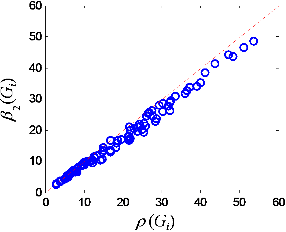
Figure 2: Scatter plot of the spectral radius, $\rho\left(G_{i}\right)$, versus the lower bound $\beta_{2}\left(G_{i}\right)$ , where each point is associated with one of the $100$ social subgraphs considered in our experiments.

From Corollary 7 and Lemma 9 we can compute the first five spectral moments of a graph $G_{i}$ from the following structural properties: number of nodes ($n_{i}$), edges ($e_{i}$), triangles ($\Delta_{i}$), quadrangles ($Q_{i}$), pentagons ($\Pi_{i}$), as well as the sum-of-squares of the degrees ($W_{i}$), and the degree-triangle correlation ($\mathcal{C}_{i}$). For convenience, we define $S\left(G_{i}\right)\triangleq\left\{n_{i},e_{i},\Delta_{i},Q_{i},\Pi_{i},W_{i},\mathcal{C}_{i}\right\}$ as a set of relevant structural properties of $G_{i}$. In our numerical experiment, we first measure the set of relevant properties $S_{i}$ for each social subgraph $G_{i}\in\mathbf{G}$, and then compute the first five spectral moments of its adjacency matrix. From these moments, we then compute the bounds $\alpha_{2}\left(G_{i}\right)$ and $\beta_{2}\left(G_{i}\right)$ using Proposition 11. As we mentioned before, these bounds can be computed as the maximum and minimum roots of a third order polynomial, for which closed form expressions are known.

We illustrate the quality of our bounds in the following figures. Fig. 2 is a scatter plot where each circle has coordinates $\left(\rho\left(G_{i}\right),\beta_{2}\left(G_{i}\right)\right)$, for all $G_{i}\in\mathbf{G}$. Observe how the spectral radii $\rho\left(G_{i}\right)$ of these social subgraphs are remarkably close to the theoretical lower bound $\beta_{2}\left(G_{i}\right)$. Therefore, we can use $\beta_{2}\left(G_{i}\right)$ as an estimate of $\rho\left(G_{i}\right)$ for social subgraphs. In Fig. 3 we include a scatter plot where each circle has coordinates $\left(-\lambda_{n}\left(G_{i}\right),-\alpha_{2}\left(G_{i}\right)\right)$, for all $G_{i}\in\mathbf{G}$. Although $\alpha_{2}\left(G_{i}\right)$ is a looser bound than $\beta_{2}\left(G_{i}\right)$, we observe how there is a strong correlation between the value of $\lambda_{n}\left(G_{i}\right)$ and $\alpha_{2}\left(G_{i}\right)$.

In these numerical experiments, we have first showed that $\alpha_{2}\left(G_{i}\right)$ and $\beta_{2}\left(G_{i}\right)$ bound the smallest and the largest eigenvalues of the adjacency matrix, and that these bounds are tight, specially $\beta_{2}\left(G_{i}\right)$. Since these bounds can be written as explicit functions of the structural properties in $S\left(G_{i}\right)$, we can estimate the impact of structural perturbations on the spectral radius and the smallest eigenvalue by studying $\left.\partial\beta_{2}\right/\partial p_{i}$ and $\left.\partial\alpha_{2}\right/\partial p_{i}$ for $p_{i}\in S\left(G_{i}\right)$. (Details of this perturbation analysis are left for future work due to space limitations.)

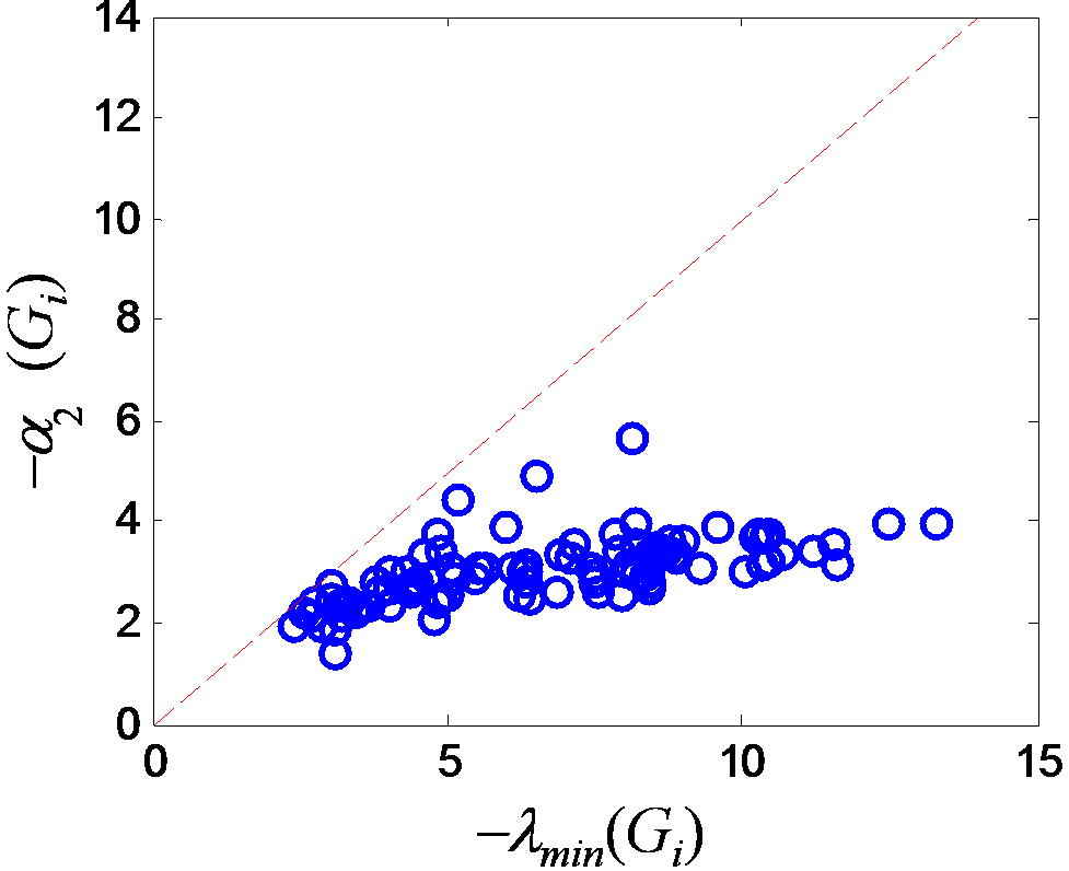
Figure 3: Scatter plot of $-\lambda_{\min}\left(G_{i}\right)$ versus the bound $-\alpha_{2}\left(G_{i}\right)$ , where each point is associated with one of the $100$ social subgraphs considered in our experiments.

VI Conclusions

In this paper, we have studied games with linear best response functions in a networked context. We have focused on analyzing the role of the network structure on the game outcome. In particular, the existence and the stability of a unique Nash equilibrium in this class of games are closely related with the smallest eigenvalue of the adjacency matrix of the network. We take this spectral result as the foundation to our work, and use algebraic graph theory and convex optimization to study how local structural properties of the network affect this eigenvalue. In particular, we have derived expressions for the first five spectral moments of the adjacency matrix in terms of local structural properties. These structural properties are: the number of nodes and edges, the number of cycles of length up to 5, the sum-of-squares of the degrees, and the degree-triangle correlation. From this sequence of five spectral moments, we propose a novel methodology to compute optimal bounds on the smallest and the largest eigenvalues of the adjacency matrix by solving two semidefinite programs. In our case, we are able to find analytical solutions to these optimal bounds by computing the roots of a cubic polynomial, for which closed-form expressions are available. Finally, we have verified the quality of our bounds by running numerical simulations in a set of 100 online social subgraphs. For future work, we shall use the results herein presented to study the effect of structural perturbations in the relevant eigenvalues of the adjacency matrix, and in properties of the Nash equilibrium.

References

- [1] D. Fudenberg and J. Tirole, Game Theory, MIT Press, 1991.
- [2] G.-M. Angeletos and A. Pavan, “Efficient Use of Information and Social Value of Information,” Econometrica, vol. 75, pp. 1103-1142, 2007.
- [3] C. Ballester, A. Calvó-Armengol, and Y. Zenou, “Who´s Who in Networks. Wanted: The Key Player,” Econometrica, vol 74, pp. 1403-1417, 2006.
- [4] Y. Bramoullé and R. Kranton, “Public Goods in Networks,” Journal of Economic Theory, vol. 135, pp. 478-494, 2007.
- [5] Y. Bramoullé, R. Kranton, and M. D’Amours, “Strategic Interaction and Networks,” CIRPEE Working Paper 10-18, 2010.
- [6] C. Ballester and A. Calvó-Armengol, “Moderate Interactions in Games with Induced Complementaries,” mimeo, Universidad Autónoma de Barcelona, 2007.
- [7] N. Biggs, Algebraic Graph Theory, Cambridge University Press, 2nd Edition, 1993.
- [8] V.M. Preciado and A. Jadbabaie, “From Local Measurements to Network Spectral Properties: Beyond Degree Distributions,” Proc. IEEE Conference on Decision and Control, 2010.
- [9] S.H. Strogatz, “Exploring Complex Networks,” Nature, vol. 410, pp. 268-276, 2001.
- [10] S. Boccaletti S., V. Latora, Y. Moreno, M. Chavez, and D.-H. Hwang, “Complex Networks: Structure and Dynamics,” Physics Reports, vol. 424, no. 4-5, pp. 175-308, 2006.
- [11] V.M. Preciado, Spectral Analysis for Stochastic Models of Large-Scale Complex Dynamical Networks, Ph.D. dissertation, Dept. Elect. Eng. Comput. Sci., MIT, Cambridge, MA, 2008.
- [12] D. Cvetković, M. Doob and H. Sachs, Spectra of Graphs, Wiley-VCH, Edition, 1998.
- [13] K.C. Das and P. Kumar, “Some New Bounds on the Spectral Radius of Graphs,” Discrete Mathematics, vol. 281, pp. 149-161, 2004.
- [14] J.B. Lasserre, “Bounding the Support of a Measure from its Marginal Moments,” Proc. AMS, in press.
- [15] J.B. Lasserre, Moments, Positive Polynomials and Their Applications, Imperial College Press, London, 2009.
- [16] http://cvxr.com/cvx/
- [17] M. Abramowitz and I.A. Stegun, Handbook of Mathematical Functions with Formulas, Graphs, and Mathematical Tables, Dover, 1965.
- [18] B. Viswanath, A. Mislove, M. Cha, and K.P. Gummadi, “On the Evolution of User Interaction in Facebook,” Proc. ACM SIGCOMM Workshop on Social Networks, 2009.
- [19] M. Stumpf, C. Wiuf, and R. May, “Subnets of Scale-Free Networks are not Scale-Free: Sampling Properties of Networks,” Proceedings of the National Academy of Sciences, vol. 102, pp. 4221-4224, 2005.