Cooperative Strategies for Simultaneous
and Broadcast Relay Channels

Abstract

Consider the simultaneous relay channel (SRC) which consists of a set of relay channels where the source wishes to transmit common and private information to each of the destinations. This problem is recognized as being equivalent to that of sending common and private information to several destinations in presence of helper relays where each channel outcome becomes a branch of the broadcast relay channel (BRC). Cooperative schemes and capacity region for a set with two memoryless relay channels are investigated. The proposed coding schemes, based on Decode-and-Forward (DF) and Compress-and-Forward (CF) must be capable of transmitting information simultaneously to all destinations in such set.

Depending on the quality of source-to-relay and relay-to-destination channels, inner bounds on the capacity of the general BRC are derived. Three cases of particular interest are considered: cooperation is based on DF strategy for both users –referred to as DF-DF region–, cooperation is based on CF strategy for both users –referred to as CF-CF region–, and cooperation is based on DF strategy for one destination and CF for the other –referred to as DF-CF region–. These results can be seen as a generalization and hence unification of previous works. An outer-bound on the capacity of the general BRC is also derived. Capacity results are obtained for the specific cases of semi-degraded and degraded Gaussian simultaneous relay channels. Rates are evaluated for Gaussian models where the source must guarantee a minimum amount of information to both users while additional information is sent to each of them.

I Introduction

The simultaneous relay channel (SRC) is defined by a set of relay channels where the source wishes to communicate common and private information to each of the destinations in the set. In order to send common information regardless of the intended channel, the source must simultaneously consider the presence of all channels as described in Fig. 1(a). This scenario offers a perspective of practical applications e.g., downlink communication on cellular networks where the base station –source– may be aided by relays and opportunistic cooperation on ad-hoc networks where the source may not be aware of the presence of a nearby relay.

Cooperative networks have been of huge interest during recent years between researchers as a possible candidate for future wireless networks [1, 2]. Using the multiplicity of information in nodes, provided by the appropriate coding strategy, these networks can increase capacity and reliability, and diversity as addressed in [3, 4, 5] where multiple relays were introduced as an antenna array using distributed space-time coding. The simplest of cooperative networks is the relay channel. First introduced in [6], it consists of a sender-receiver pair whose communication is aided by a relay node. In other words, it consists of a channel input $X$, a relay input $X_{1}$, a channel output $Y_{1}$ and a relay output $Z_{1}$, where the relay input depends only on the past observations. A significant contribution was made by Cover and El Gamal [7], where the main strategies of Decode-and-Forward (DF) and Compress-and-Forward (CF), and a max-flow min-cut upper bound were developed for this channel. Moreover the capacity of the degraded and the reversely degraded relay channel were established by the authors. A general theorem that combines DF and CF in a single coding scheme was also presented. The capacity of semi-deterministic relay channels and the capacity of cascaded relay channels were found in [8, 9]. A converse for the relay channel has been developed in [10]. The capacity of orthogonal relay channels was found in [11] while the relay channel with private messages was discussed in [12]. The capacity of a class of modulo-Sum relay channels was also found in [13]. More recently, Compute-and-Forward strategy based on (linear) structured coding was proposed in [14]. It has been shown that the use of lattice codes outperforms DF strategy in some settings.

In general, the performance of DF and CF schemes are directly related to the noise condition between the relay and the destination. More precisely, it is well-known that DF scheme performs much better than CF when the source-to-relay channel is quite strong. Whereas CF scheme is more suitable when the relay-to-destination channel is strong. Indeed, inner bounds based on DF and CF strategies can be obtained using different coding and decoding techniques. Coding techniques can be classified [15] into regular and irregular coding. Irregular coding exploits the codebooks of different sizes that are involved between relay and source while regular coding requires the same size. Decoding techniques also can roughly be classified into successive and simultaneous decoding. Successive decoding method decodes the transmitted codebooks in a consecutive manner. In each block, the decoder starts with a group of codebooks (e.g. relay codewords) and then afterward it moves to the next group (e.g. source codewords). However, simultaneous decoding decodes jointly all codebooks in a given block. Generally speaking, the latter provides the better results than the former. Cover and El Gamal [7] have proposed irregular coding with successive decoding. In fact, regular coding with simultaneous decoding was first developed in [16]. It can be exploited for decoding with the channel outputs of a single or multiple blocks. For instance, the author in [17] by relying on this property introduces the notion of sliding window decoding to perform decoding based on the outputs of two consecutive blocks. The notion of backward decoding was proposed in [18] and it consists of a decoder who waits until the last block to start decoding from the last to the first message. Backward coding is shown to provide better performances than other schemes based on simultaneous decoding [19, 20] such as sliding window. Backward decoding can use a single block as in [18] or multiple blocks as in [21] to perform decoding. The best known lower bound on the capacity of the relay channel was derived in [22], by using a generalized backward decoding strategy.

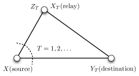
(a) Simultaneous relay channel (SRC)

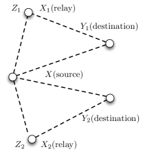
(b) BRC with two relays

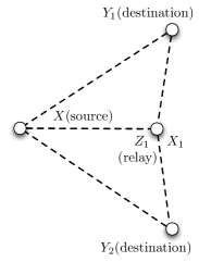
(c) BRC with common relay

Figure 1: Simultaneous and broadcast relay channels.

Extension to multiple relay networks have been studied in [23] and practical scenarios were also considered, like the Gaussian relay channel[24, 25, 26], and the Gaussian parallel relay network [27, 28, 29]. The combination of the relay channel with other networks has been studied. The multiple access relay channel (MARC) was analyzed in [30, 31, 32]. The relay-broadcast channel (RBC) where a user which can be either the receiver or a distinct node, serves as a relay for transmitting the information to the receivers, was also studied. An achievable rate region for the dedicated RBC was obtained in [15]. Preliminary works on the RBC were done in [33, 34, 35] and the capacity region of physically degraded RBC was found in [36]. Inner and outer rate regions for the RBC were developed further in [37, 38, 39]. The capacity of Gaussian dedicated RBC with degraded relay channel was reported in [40].

Compound channels were introduced and further investigated in [41, 42, 43]. Extensive research has been undertaken for years (see [44] and references therein). This class of channels model communications over a set of possible channels where the encoder aims to maximize the worst-case capacity. Actually, the compound relay channel has a similar definition to the SRC. The SRC guarantees common and private rates for every channel in the set while the compound relay channel only guarantees a common rate. However, both terms are kept throughout this paper to indicate the difference in the code definition utilized with each model. An interesting relation between compound and broadcast channels was first mentioned in [45], where it was suggested that the compound channel problem can be investigated via the broadcast channel. Indeed, this concept of broadcasting has been used as a method to mitigate the effect of channel uncertainty in numerous contributions [46, 21, 47, 48, 49]. Moreover, the SRC was also investigated through broadcast channels in [50, 51, 52]. This strategy facilitates rate adaptation to the current channel in operation without requiring feedback information from the destination to the transmitter.

The broadcast channel (BC) was introduced in [45] along with the capacity of binary symmetric, product, push-to-talk and orthogonal BCs. The capacity of the degraded BC was established in [53, 54, 55, 56]. It was shown that feedback does not increase capacity of physically degraded BCs [57, 58], but it does for Gaussian BCs [59]. The capacity of the BC with degraded message sets was found in [60] while that of more capable and less-noisy were established in [61]. The best known inner bound for general BCs is due to Marton [62] and an alternative proof was given in [63] (see [64] and reference therein). This inner bound was shown to be tight for channels with one deterministic component [65] and deterministic channels [66, 67]. An outer-bound for the general BC was established in [62] and improved later in [68, 69].

In this paper, we study different coding strategies and capacity region for the general memoryless broadcast relay channel (BRC) with two relays and destinations, as depicted in Fig. 1(b). This model is equivalent to the SRC with two simultaneous memoryless relay channels. It should be emphasized that, by adding adequate Markov chains such that relays only affect a single destination, the BRC can be considered as being equivalent to the SRC. Nevertheless, for sake of generality we will not explicitly constrain the results trough this paper to the SRC. The rest of the paper is organized as follows. Section II introduces the main definitions and the problem statement. Inner bounds on the capacity region are derived for three cases of particular interest:

• Source-to-relay channels are stronger than the others and hence cooperation is based on DF strategy for both users (referred to as DF-DF region), corresponding to the SRC with DF relays.

• Relay-to-destination channels are stronger than the others and hence cooperation is based on CF strategy for both users (referred to as as CF-CF region), corresponding to the SRC with CF relays.

• The source-to-relay channel of one destination is stronger than its corresponding relay-to-destination channel. Whereas for the other destination the relay-to-destination channel is stronger than its source-to-relay channel. Hence cooperation is based on DF strategy for one destination and CF for the other one (referred to as DF-CF region). This case corresponds to the SRC where a different coding strategy is employed at each relay.

Section III examines general outer-bounds and capacity results for several classes of BRCs. In particular, the case of the broadcast relay channel with common relay (BRC-CR) is investigated, as shown in Fig. 1(c). We show that the DF-DF region improves existent results [15] on BRC-CR. Capacity results are obtained for the specific cases of semi-degraded and degraded Gaussian simultaneous relay channels. In Section IV, rates are computed for the case of distant based additive white Gaussian noise (AWGN) relay channels. Achievability and converse proofs are relegated to the appendices while summary and discussion are presented in Section V.

Notation

For any sequence $(x_{i})_{i\in\mathbb{N}_{+}}$, notation $\underline{x}$ stands for the collection $x_{1}^{n}=(x_{1},x_{2},\dots,x_{n})$. Entropy is denoted by $H(\cdot)$, and mutual information by $I(\cdot;\cdot)$. The differential entropy function is denoted by $h(\cdot)$. We denote $\epsilon$-typical and conditional $\epsilon$-typical sets by $\textsl{A}^{n}_{\epsilon}(X)$ and $\textsl{A}^{n}_{\epsilon}(Y|X)$, respectively (see [70] for details). Let $X$, $Y$ and $Z$ be three random variables on some alphabets with probability distribution $p$. If $p(x|yz)=p(x|y)$ for each $x,y,z$, then they form a Markov chain, denoted by $X-\!\!\!\!\minuso\!\!\!\!-Y-\!\!\!\!\minuso\!\!\!\!-Z$. Logarithms are taken in base $2$ and denoted by $\log(\cdot)$. The capacity function is defined as $\mathcal{C}(x)=\frac{1}{2}\log(1+x)$.

II Main Definitions and Achievable Regions

In this section, we first formalize the problem of the simultaneous relay channel and then present achievable rate regions for the cases of DF-DF strategy (DF-DF region), CF-CF strategy (CF-CF region) and DF-CF strategy (DF-CF region).

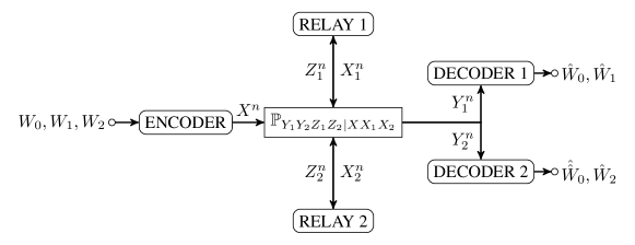
Figure 2: Broadcast relay channel (BRC).

II-A Problem statement

The simultaneous relay channel [50] with discrete source and relay inputs $x\in\mathcal{X}$, $x_{T}\in\mathcal{X}_{T}$, discrete channel and relay outputs $y_{T}\in\mathcal{Y}_{T}$, $z_{T}\in\mathcal{Z}_{T}$, is characterized by a set of relay channels, each of them defined by a conditional probability distribution (PD)

$$\mathcal{P}_{\textrm{SRC}}=\left\{P_{Y_{T}Z_{T}|XX_{T}}:\mathcal{X}\times\mathcal{X}_{T}\longmapsto\mathcal{Y}_{T}\times\mathcal{Z}_{T}\right\},$$

where $T$ denotes the channel index. The SRC models the situation in which only one single channel is present at once, but it does not change during the communication. However, the transmitter is not cognizant of the realization of $T$ governing the communication. In this setting, $T$ is assumed to be known at the destination and the relay ends. The transition PD of the $n$-memoryless extension with inputs $(\mathbf{x},\mathbf{x}_{T})$ and outputs $(\mathbf{y}_{T},\mathbf{z}_{T})$ is given by

$$P^{n}_{Y_{T}Z_{T}|XX_{T}}(\mathbf{y}_{T},\mathbf{z}_{T}|\mathbf{x},\mathbf{x}_{T})=\prod\limits_{i=1}^{n}P_{T}(y_{T,i},z_{T,i}|x_{i},x_{T,i}).$$

The focus is on the case where ${T=\{1,2\}}$, in other words there are two relay channels in the set.

Definition 1 (code)

A code for the SRC consists of:

• An encoder mapping $\{\varphi:\mathcal{W}_{0}\times\mathcal{W}_{1}\times\mathcal{W}_{2}\longmapsto\mathcal{X}^{n}\}$,

• Two decoder mappings $\{\psi_{T}:\mathcal{Y}_{T}^{n}\longmapsto\mathcal{W}_{0}\times\mathcal{W}_{T}\}$,

• A set of relay functions $\{f_{T,i}\}_{i=1}^{n}$ such that

  $$\{f_{T,i}:\mathcal{Z}_{T}^{i-1}\longmapsto\mathcal{X}_{T}^{n}\}_{i=1}^{n},$$

for $T=\{1,2\}$ and some finite sets of integers $\mathcal{W}_{b}=\big{\{}1,\dots,M_{b}\big{\}}_{b=\{0,1,2\}}$. The rates of such code are $n^{-1}\log M_{b}$ and the corresponding maximum error probabilities for $T=\{1,2\}$ are defined as

$$P_{e,T}^{(n)}\big{(}\varphi,\psi, \{f_{T,i}\}_{i=1}^{n}\big{)}=$$

$$\max_{(w_{0},w_{T})\in\mathcal{W}_{0}\times\mathcal{W}_{T}}\Pr\left\{\psi(\mathbf{Y}_{T})\neq(w_{0},w_{T})\right\}.$$

Definition 2 (achievability and capacity)

For any positive numbers $0<\epsilon,\gamma<1$, a triple of non-negative numbers $(R_{0},R_{1},R_{2})$ is said achievable for the SRC if for every sufficiently large $n$, there exists a $n$-length block code whose error probability satisfies

$$P_{e,T}^{(n)}\big{(}\varphi,\psi,\{f_{T,i}\}_{i=1}^{n}\big{)}\leq\epsilon$$

for $T=\{1,2\}$ and the rates $\frac{1}{n}\log M_{b}\geq R_{b}-\gamma$ for $b=\{0,1,2\}$. The set of all achievable rates $\mathcal{C}_{\textrm{SRC}}$ is called the capacity region of the SRC. We emphasize that no prior distribution on $T$ is assumed and thus the encoder must exhibit a code that yields small error probability for every $T=\{1,2\}$. A similar definition can be offered for the common-message SRC with a single message set $\mathcal{W}_{0}$, $n^{-1}\log M_{0}$ and rate $R_{0}$. The common-message SRC is equivalent to the compound relay channel and so its achievable rate is similarly defined.

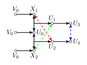
(a) Diagram of auxiliary random variables

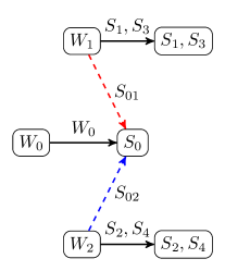
(b) Message reconfiguration

Figure 3: Description of encoding techniques for DF strategy.

 

$$I_{i}= \min\big{\{}I(U_{0},U_{i};Z_{i}|V_{0},X_{i})+I(U_{i+2};Y_{i}|U_{0},V_{0},X_{i},U_{i}),I(U_{0},V_{0},U_{i},U_{i+2},X_{i};Y_{i})\big{\}},$$

$$J_{i}= \min\big{\{}I(U_{i};Z_{i}|U_{0},V_{0},X_{i})+I(U_{i+2};Y_{i}|U_{0},V_{0},X_{i},U_{i}),I(U_{i+2},U_{i},X_{i};Y_{i}|U_{0},V_{0})\big{\}},$$

$$I_{M}= I(U_{3};U_{4}|U_{1},U_{2},X_{1},X_{2},U_{0},V_{0}),$$ (1)

 

$$\begin{array}[]{c}\\ \mathcal{Q}=\big{\{}P_{U_{0}V_{0}U_{1}U_{2}U_{3}U_{4}X_{1}X_{2}X}=P_{U_{3}U_{4}X|U_{1}U_{2}}P_{U_{1}U_{2}|U_{0}X_{1}X_{2}}\,P_{U_{0}|X_{1}X_{2}V_{0}}P_{X_{2}|V_{0}}P_{X_{1}|V_{0}}P_{V_{0}}\vspace{1mm}\\ \textrm{ satisfying }\\ \vspace{1mm}(U_{0},V_{0},U_{1},U_{2},U_{3},U_{4})-\!\!\!\!\minuso\!\!\!\!-(X_{1},X_{2},X)-\!\!\!\!\minuso\!\!\!\!-(Y_{1},Z_{1},Y_{2},Z_{2})\big{\}}.\end{array}$$ (2)

Remark 1

We emphasize that both relay and destination are assumed to be cognizant of the realization of $T$ and hence the problem of coding for the SRC can be turned into that of the broadcast relay channel (BRC) [50]. Because the source is uncertain about the actual channel, it has to count for each of them and therefore assume the simultaneous presence of both. This leads to an equivalent broadcast model consisting of two sub-channels (or branches) for $T=\{1,2\}$, where each one corresponds to a single-relay channel, as illustrated in Fig. 1(b) and Fig. 2. The encoder sends common and private messages $(W_{0},W_{T})$ to destination $T$ at rates $(R_{0},R_{T})$. The general BRC is defined by the PD

$$\mathcal{P}_{\textrm{BRC}}=\Big{\{} \mathbb{P}_{Y_{1}Z_{1}Y_{2}Z_{2}|XX_{1}X_{2}}:$$

$$\mathcal{X}\times\mathcal{X}_{1}\times\mathcal{X}_{2}\longmapsto\mathcal{Y}_{1}\times\mathcal{Z}_{1}\times\mathcal{Y}_{2}\times\mathcal{Z}_{2}\Big{\}},$$

with channel and relay inputs $(X,X_{1},X_{2})$ and channel and relay outputs $(Y_{1},Z_{1},Y_{2},Z_{2})$. Notions of achievability for rates $(R_{0},R_{1},R_{2})$ and capacity remain the same as for conventional BCs (see [45], [15] and [37]). Similar to the case of conventional BCs, the capacity region of the BRC depends only on the marginal PDs: $P_{Y_{1}|XX_{1}X_{2}Z_{1}Z_{2}}$, $P_{Y_{2}|XX_{1}X_{2}Z_{1}Z_{2}}$ and $P_{Z_{1}Z_{2}|XX_{1}X_{2}}$.

Remark 2

The definition of the BRC does not dismiss the possibility of dependence of destination $Y_{1}$ (respect to destination $Y_{2}$) on the relay input $X_{2}$ (respect to the relay input $X_{1}$). Therefore, it appears to be more general than the SRC. In other words, the current definition of BRC corresponds to that of the SRC with the additional constraints that $(Y_{1},Z_{1})-\!\!\!\!\minuso\!\!\!\!-(X,X_{1})-\!\!\!\!\minuso\!\!\!\!-(Y_{2},Z_{2},X_{2})$ and $(Y_{2},Z_{2})-\!\!\!\!\minuso\!\!\!\!-(X,X_{2})-\!\!\!\!\minuso\!\!\!\!-(Y_{1},Z_{1},X_{1})$. These Markov chains guarantee that $(Y_{T},Z_{T})$ only depend on inputs $(X,X_{T})$, for $T=\{1,2\}$. Despite the fact that this condition is not necessary until converse proofs, the achievable region developed below are more adapted to the SRC. Nevertheless, these achievable rate regions do not require any additional assumption and thus are valid for the general BRC as well.

The next subsections provide achievable rate regions for three different coding strategies.

II-B Achievable region based on DF-DF strategy

Consider the situation where the source-to-relay channels are stronger than the others. In this case, the best known coding strategy for both relays turns out to be Decode-and-Forward (DF). The source should broadcast the information to the destinations based on a broadcast code combined with DF scheme. Both relays help the common information using a common description, namely $V_{0}$. The private information for each destination is sent partly by the help of the corresponding relay and partly by direct transmission. The next theorem presents the achievable rate region [52].

Theorem 1

(DF-DF region) An inner bound on the capacity region $\mathcal{R}_{\textrm{DF-DF}}\subseteq\mathcal{C}_{\textrm{BRC}}$ of the broadcast relay channel is given by

$$\mathcal{R}_{\textrm{DF-DF}}=\displaystyle{co\bigcup\limits_{P\in\mathcal{Q}}} \Big{\{}(R_{0}\geq 0,R_{1}\geq 0,R_{2}\geq 0):$$

$$R_{0}+R_{1}\leq I_{1}-I(U_{0},U_{1};X_{2}|X_{1},V_{0}),$$

$$R_{0}+R_{2}\leq I_{2}-I(U_{0},U_{2};X_{1}|X_{2},V_{0}),$$

$$R_{0}+R_{1}+R_{2}\leq I_{1}+J_{2}-I(U_{0},U_{1};X_{2}|X_{1},V_{0})$$

$$-I(U_{1},X_{1};U_{2}|X_{2},U_{0},V_{0})-I_{M}$$

$$R_{0}+R_{1}+R_{2}\leq J_{1}+I_{2}-I(U_{0},U_{2};X_{1}|X_{2},V_{0})$$

$$-I(U_{1};U_{2},X_{2}|X_{1},U_{0},V_{0})-I_{M}$$

$$2R_{0}+R_{1}+R_{2}\leq I_{1}+I_{2}-I(U_{0},U_{1};X_{2}|X_{1},V_{0})$$

$$-I(U_{0},U_{2};X_{1}|X_{2},V_{0})$$

$$-I(U_{1};U_{2}|X_{1},X_{2},U_{0},V_{0})-I_{M}\Big{\}},$$

where $(I_{i},J_{i},I_{M})$ with $i=\{1,2\}$ are as in (1). $co\{\cdot\}$ denotes the convex hull and the union is over all joint PDs $P_{U_{0}V_{0}U_{1}U_{2}U_{3}U_{4}X_{1}X_{2}X}\in\mathcal{Q}$, with $\mathcal{Q}$ given by (2).

Proof:

The proof of this theorem is relegated to Appendix A. Instead, here we provide an overview of it. First, the original messages are reorganized via rate-splitting into new messages, as shown in Fig. 3(b), where we add part of the private messages together with the common message into new messages, which is similarly to [15]. The general coding idea of the proof is depicted in Fig. 3(a).

The description $V_{0}$ represents the common part of $(X_{1},X_{2})$ (the information sent by the relays), which is intended to help the common information encoded in $U_{0}$. Private information is sent in two steps, first using the relay help through $(U_{1},U_{2})$ and based on DF strategy. Then, the direct links between source and destinations are used to decode $(U_{3},U_{4})$. Marton coding is used to allow correlation between the descriptions according to the arrows in Fig. 3(a). To make a random variable simultaneously correlated with multiple random variables (RVs), we used multi-level Marton coding.

TABLE I: DF strategy with $b=\{1,2\}$

$\underline{v}_{0}(t_{0(i-1)})$	$\underline{v}_{0}(t_{0(i)})$
$\underline{u}_{0}(t_{0(i-1)},t_{0i})$	$\underline{u}_{0}(t_{0i},t_{0(i+1)})$
$\underline{x}_{b}(t_{0(i-1)},t_{b(i-1)})$	$\underline{x}_{b}(t_{0i},t_{bi})$
$\underline{u}_{b}(t_{0(i-1)},t_{0i},t_{b(i-1)},t_{bi})$	$\underline{u}_{b}(t_{0i},t_{0(i+1)},t_{bi},t_{b(i+1)})$
$\underline{u}_{b+2}(t_{0(i-1)},t_{0i},t_{b(i-1)},t_{bi},t_{(b+2)i})$	$\underline{u}_{b+2}(t_{0i},t_{0(i+1)},t_{bi},t_{b(i+1)},t_{(b+2)(i+1)})$
$\underline{y}_{bi}$	$\underline{y}_{b(i+1)}$

Full details for this process are explained in Appendix A while Table I shows details for the transmission in time. Both relays knowing $(\underline{v}_{0},\underline{x}_{b})$ decode $(\underline{u}_{0},\underline{u}_{b})$ in the same block. Then each destination, by using backward decoding, decodes all codebooks in the last block. The final region is a combination of all constraints from Marton coding and decoding, which reduce to the above region by using Fourier-Motzkin elimination. ∎

Remark 3

We have the following observations:

• The rates in Theorem 1 coincide with the conventional rate based on partial DF [7], and moreover it is easy to verify that, by setting $(X_{1},X_{2},V_{0})=\emptyset$, $U_{3}=U_{1},U_{4}=U_{2}$ $Z_{1}=Y_{1}$ and $Z_{2}=Y_{2}$, the rate region in Theorem 1 is equivalent to Marton’s region [62],

• The new region improves on the existent regions for the general BRC in [50] and for the BRC with common relay as depicted in Fig. 1(c). By setting $X_{1}=X_{2}=V_{0}$ and $U_{1}=U_{2}=U_{0}$, the rate region in Theorem 1 can be shown to be equivalent to the inner bound in [15]. Whereas the next corollary shows that the novel rate region is strictly large than that in [15].

The following corollary provides a sharper inner bound on the capacity region of the BRC with common relay (BRC-CR). By dividing the help of relay into two components $V_{0}$ and $X_{1}$, the relay is also able to help private information of the first destination. This is in contrast to the encoding technique used in [15], where the relay only helps common information. As a consequence of this, when $Y_{2}=\emptyset$ and the first destination is a physically degraded version of the relay the region in [15] cannot achieve the capacity of this channel. This is not the case of the next rate region. Furthermore, it will be shown later that a special case of this corollary reaches the capacity of the degraded Gaussian BRC-CR and semi-degraded BRC-CR.

Corollary 1 (BRC with common relay)

An inner bound on the capacity region of the BRC-CR $\mathcal{R}_{\textrm{BRC-CR}}\subseteq$ $\mathcal{C}_{\textrm{BRC-CR}}$ is given by

$$\mathcal{R}_{\textrm{BRC-CR}}=co \displaystyle{\bigcup\limits_{P_{V_{0}U_{0}U_{1}U_{3}U_{4}X_{1}X}\in\mathcal{Q}}}\Big{\{}$$

$$(R_{0}\geq 0,R_{1}\geq 0, R_{2}\geq 0):$$

$$R_{0}+R_{1} \leq\min\{I_{1}+I_{1p},I_{3}+I_{3p}\}$$

$$+I(U_{3};Y_{1}|U_{1},U_{0},X_{1},V_{0}),$$

$$R_{0}+R_{2} \leq I(U_{0},V_{0},U_{4};Y_{2})-I(U_{0};X_{1}|V_{0}),$$

$$R_{0}+R_{1}+R_{2} \leq\min\{I_{2},I_{3}\}+I_{3p}$$

$$+I(U_{3};Y_{1}|U_{1},U_{0},X_{1},V_{0})$$

$$+I(U_{4}; Y_{2}|U_{0},V_{0})-I(U_{0};X_{1}|V_{0})-I_{M},$$

$$R_{0}+R_{1}+R_{2} \leq\min\{I_{1},I_{3}\}+I_{1p}$$

$$+I(U_{3};Y_{1}|U_{1},U_{0},X_{1},V_{0})$$

$$+I(U_{4}; Y_{2}|U_{0},V_{0})-I(U_{0};X_{1}|V_{0})-I_{M},$$

$$2R_{0}+R_{1}+R_{2} \leq I(U_{3};Y_{1}|U_{1},U_{0},X_{1},V_{0})$$

$$+I(U_{4};Y_{2}|U_{0},V_{0})+I_{2}$$

$$+\min\{I_{1}+I_{1p},I_{3}+I_{3p}\}$$

$$-I(U_{0};X_{1}|V_{0})-I_{M}\Big{\}}$$

where the quantities are defined by

$$I_{1} =I(U_{0},V_{0};Y_{1}),$$

$$I_{2} =I(U_{0},V_{0};Y_{2}),$$

$$I_{3} =I(U_{0};Z_{1}|X_{1},V_{0}),$$

$$I_{1p} =I(U_{1}X_{1};Y_{1}|U_{0},V_{0}),$$

$$I_{3p} =I(U_{1};Z_{1}|U_{0},V_{0},X_{1}),$$

$$I_{M} =I(U_{3};U_{4}|X_{1},U_{1},U_{0},V_{0}),$$

$co\{\cdot\}$ denotes the convex hull and $\mathcal{Q}$ is the set of all joint PDs $P_{V_{0}U_{0}U_{1}U_{3}U_{4}X_{1}X}$ satisfying

$$\begin{array}[]{c}(V_{0},U_{0},U_{1},U_{3},U_{4})-\!\!\!\!\minuso\!\!\!\!-(X_{1},X)-\!\!\!\!\minuso\!\!\!\!-(Y_{1},Z_{1},Y_{2}).\end{array}$$

II-C Achievable region based on CF-DF strategy

Consider now a broadcast relay channel where the source-to-relay channel is stronger that the relay-to-destination channel for the first user and weaker for the second one. Hence cooperation is better be based on DF scheme for user one and CF scheme for user two. Actually, the source must broadcast the information to the destinations based on a broadcast code combined with CF and DF schemes. This scenario may arise when the encoder does not know (e.g. due to user mobility and fading) whether the source-to-relay channel is much stronger or not than the relay-to-destination channel. The next theorem presents the general achievable rate region for the case where the first relay employs DF scheme while the second relay uses CF scheme to help common and private information [71].

Theorem 2 (CF-DF region)

An inner bound on the capacity region of the BRC $\mathcal{R}_{\textrm{DF-CF}}\subseteq\mathcal{C}_{\textrm{BRC}}$ with heterogeneous cooperative strategies is given by

$$\mathcal{R}_{\textrm{CF-DF}} =co\displaystyle{\bigcup\limits_{P\in\mathcal{Q}}}\Big{\{}(R_{0}\geq 0,R_{1}\geq 0,R_{2}\geq 0):$$

$$R_{0}+R_{1} \leq I_{1},$$

$$R_{0}+R_{2} \leq I_{2}-I(U_{2};X_{1}|U_{0},V_{0}),$$

$$R_{0}+R_{1}+R_{2} \leq I_{1}+J_{2}-I(U_{1},X_{1};U_{2}|U_{0},V_{0}),$$

$$R_{0}+R_{1}+R_{2} \leq J_{1}+I_{2}-I(U_{1},X_{1};U_{2}|U_{0},V_{0}),$$

$$2R_{0}+R_{1}+R_{2} \leq I_{1}+I_{2}-I(U_{1},X_{1};U_{2}|U_{0},V_{0})\Big{\}},$$

where the quantities $(I_{i},J_{i},\Delta_{0})$ with $i=\{1,2\}$ are given by

$$I_{1} =\min\big{\{}I(U_{0},U_{1};Z_{1}|X_{1},V_{0}),I(U_{1},U_{0},X_{1},V_{0};Y_{1})\big{\}},$$

$$I_{2} =I(U_{2},U_{0},V_{0};\hat{Z}_{2},Y_{2}|X_{2}),$$

$$J_{1} =\min\big{\{}I(U_{1};Z_{1}|X_{1},U_{0},V_{0}),I(U_{1},X_{1};Y_{1}|U_{0},V_{0})\big{\}},$$

$$J_{2} =I(U_{2};\hat{Z}_{2},Y_{2}|X_{2},U_{0},V_{0}),$$

$co\{\cdot\}$ denotes the convex hull and the set of all admissible PDs $\mathcal{Q}$ is defined as

$$\mathcal{Q}=\Big{\{} P_{V_{0}U_{0}U_{1}U_{2}X_{1}X_{2}XY_{1}Y_{2}Z_{1}Z_{2}\hat{Z}_{2}}=P_{V_{0}}P_{X_{2}}P_{X_{1}|V_{0}}$$

$$P_{U_{0}|V_{0}}P_{U_{2}U_{1}|X_{1}U_{0}}P_{X|U_{2}U_{1}}P_{Y_{1}Y_{2}Z_{1}Z_{2}|XX_{1}X_{2}}\times$$

$$P_{\hat{Z}_{2}|X_{2}Z_{2}},\,\,\,$$

$$\textrm{satisfying }\,\,\,I(X_{2};Y_{2})\geq I(Z_{2};\hat{Z}_{2}|X_{2}Y_{2})\,\,\,\textrm{and }$$

$$(V_{0}, U_{0},U_{1},U_{2})-\!\!\!\!\minuso\!\!\!\!-(X_{1},X_{2},X)-\!\!\!\!\minuso\!\!\!\!-(Y_{1},Z_{1},Y_{2},Z_{2})\Big{\}}.$$

Remark 4

It should emphasized that it is possible to exchange the coding strategy between first and second relay and thus a bigger region is obtained by taking the convex hull of the union of both regions.

The proof of this theorem is relegated to Appendix B. Instead, here we discuss the relevant steps of it. In order to send common information while exploiting the help of DF relay at destination 1, we use regular encoding with block-Markov coding. The description $V_{0}$ is the part of $X_{1}$ to help the transmission of $U_{0}$, and the second relay helps destination 2 based on CF scheme (i.e. relay and source inputs are independently chosen). Regular encoding is used to superimpose the code of the current block over that of the previous block. The relay using DF scheme transmits the message from the previous block and hence the destination can exploit it for decoding as usually. But the relay using CF scheme seems to impose the decoding of two superimposed codes at the destination. By noting that the codeword center carries the dummy message in the first block, the destination decodes the cloud knowing the center, and then in the next block it continues by removing the center code.

Nevertheless, this procedure leads to performance loss because one part of the transmitted code is indeed thrown away. Therefore, at this point the reader may think that superposition coding needed for DF should not work with CF scheme. Helpfully, this is not the case. By using backward decoding, the code can be exploited with CF scheme as well and without loss of performance. The destination decoding CF scheme takes $V_{0}$ not as the relay code but as part of the source code, over which $U_{0}$ is superimposed. Then, the last block $U_{0}$ carries the dummy message superimposed on $V_{0}$, which is the message from the last block. For instance, $(U_{0},V_{0})$ can be jointly decoded by exploiting both codes and without performance loss with respect to usual CF scheme.

Finally, we consider the compound relay channel, where the channel in operation is chosen from the set of relay channels. For simplicity, suppose that the set includes only two channels such that DF compared to CF strategy yields a better rate for the first channel and a worse rate for the second one. The overall goal is to transmit at the best possible rate with arbitrary small error probability for both channels. Then using regular encoding, it can be seen that the best cooperative strategy can be selected for each channel because the first relay employs DF while the second one uses CF scheme. The next corollary directly results from this observation.

Corollary 2 (common-information)

A lower bound on the capacity of the compound relay channel (or common-message BRC) is given by all rates $R_{0}$ satysfing

$$\begin{array}[]{rl}R_{0}\leq\max\limits_{P_{X_{1}X_{2}X}\in\mathcal{Q}}&\min\big{\{}I(X;Z_{1}|X_{1}),\\ &I(X,X_{1};Y_{1}),I(X;\hat{Z}_{2},Y_{2}|X_{2})\big{\}}.\end{array}$$

Corollary 3 (private information)

An inner bound on the capacity region of the BRC with heterogeneous cooperative strategies is given by the convex hull of the set of rates $(R_{1},R_{2})$ satisfying

$$R_{1} \leq\min\big{\{}I(U_{1};Z_{1}|X_{1}),I(U_{1},X_{1};Y_{1})\big{\}},$$

$$R_{2} \leq I(U_{2};\hat{Z}_{2},Y_{2}|X_{2})-I(U_{2};X_{1}),$$

$$R_{1}+R_{2} \leq\min\big{\{}I(U_{1};Z_{1}|X_{1}),I(U_{1},X_{1};Y_{1})\big{\}}$$

$$+I(U_{2};\hat{Z}_{2},Y_{2}|X_{2})-I(U_{1},X_{1};U_{2}),$$

for all joint PDs $P_{U_{1}U_{2}X_{1}X_{2}XY_{1}Y_{2}Z_{1}Z_{2}\hat{Z}_{2}}\in\mathcal{Q}$.

Corollary 2 follows from Theorem 2 by choosing $U_{1}=U_{2}=U_{0}=X$, $V_{0}=X_{1}$. Whereas Corollary 3 follows by setting $U_{0}=V_{0}=\emptyset$.

Remark 5

The region in Theorem 2 is equivalent to Marton’s region [62] with $(X_{1},X_{2},V_{0})=\emptyset$, $Z_{1}=Y_{1}$ and $Z_{2}=Y_{2}$. Observe that the rate corresponding to DF scheme which appears in Theorem 2 coincides with the usual DF rate, whereas the CF rate appears with a little difference. In fact, $X$ is being decomposed into $(U,X_{1})$, replacing it in the rate term corresponding to CF scheme.

II-D Achievable region based on CF-CF strategy

Consider now another scenario where both relay-to-destination channels are stronger than the others and hence the efficient coding strategy turns to be CF scheme for both users. The inner bound based on this strategy is stated in the following theorem [72] and its proof is presented in Appendix C.

Theorem 3 (CF-CF region)

An inner bound on the capacity region of the BRC $\mathcal{R}_{\textrm{CF-CF}}\subseteq\mathcal{C}_{\textrm{BRC}}$ is given by

$$\mathcal{R}_{\textrm{CF-CF}}=co\displaystyle{\bigcup\limits_{P\in\mathcal{Q}}}\Big{\{}(R_{0} \geq 0,R_{1}\geq 0,R_{2}\geq 0):$$

$$R_{0}+R_{1} \leq I(U_{0},U_{1};Y_{1},\hat{Z}_{1}|X_{1}),$$

$$R_{0}+R_{2} \leq I(U_{0},U_{2};Y_{2},\hat{Z}_{2}|X_{2}),$$

$$R_{0}+R_{1}+R_{2} \leq I_{0}+I(U_{1};Y_{1},\hat{Z}_{1}|X_{1},U_{0})$$

$$+I(U_{2};Y_{2} ,\hat{Z}_{2}|X_{2},U_{0})-I(U_{1};U_{2}|U_{0}),$$

$$2R_{0}+R_{1}+R_{2} \leq I(U_{0},U_{1};Y_{1},\hat{Z}_{1}|X_{1})$$

$$+I(U_{0},U_{2} ;Y_{2},\hat{Z}_{2}|X_{2})-I(U_{1};U_{2}|U_{0})\Big{\}},$$

where the quantity $I_{0}$ is defined by

$$\begin{array}[]{l}I_{0}=\min\big{\{}I(U_{0};Y_{1},\hat{Z}_{1}|X_{1}),I(U_{0};Y_{2},\hat{Z}_{2}|X_{2})\big{\}},\\ \end{array}$$

$co\{\cdot\}$ denotes the convex hull and the set of all admissible PDs $\mathcal{Q}$ is defined as

$$\mathcal{Q}=\big{\{} P_{U_{0}U_{1}U_{2}X_{1}X_{2}XY_{1}Y_{2}Z_{1}Z_{2}\hat{Z}_{1}\hat{Z}_{2}}=P_{X_{2}}P_{X_{1}}P_{U_{0}}\times$$

$$P_{U_{2}U_{1}|U_{0}}P_{X|U_{2}U_{1}}P_{Y_{1}Y_{2}Z_{1}Z_{2}|XX_{1}X_{2}}\times$$

$$P_{\hat{Z}_{1}|X_{1}Z_{1}}P_{\hat{Z}_{2}|X_{2}Z_{2}},$$

$$I(X_{1};Y_{1})\geq I(Z_{1};\hat{Z}_{1}|X_{1},Y_{1}),$$

$$I(X_{2};Y_{2})\geq I(Z_{2};\hat{Z}_{2}|X_{2},Y_{2}),$$

$$(U_{0},U_{1},U_{2})-\!\!\!\!\minuso\!\!\!\!-(X_{1},X_{2},X)-\!\!\!\!\minuso\!\!\!\!-(Y_{1},Z_{1},Y_{2},Z_{2})\big{\}}.$$

Notice that by setting $(X_{1},X_{2})=\emptyset$, $Z_{1}=Y_{1}$ and $Z_{2}=Y_{2}$ this region is equivalent to Marton’s region [62].

Remark 6

A general achievable rate region follows by applying time-sharing on the regions stated in Theorems 1, 2 and 3.

III Outer Bounds and Capacity Results

In this section, we first provide an outer-bound on the capacity region of the general BRC . Then some capacity results for the cases of semi-degraded BRC with common relay (BRC-CR) and degraded Gaussian BRC-CR are stated.

III-A Outer bounds on the capacity region of general BRC

The next theorems provide general outer-bounds on the capacity regions of the BRC described in Fig. 2 and the BRC-CR where $X_{1}=X_{2}$ and $Z_{1}=Z_{2}$, respectively. The proof is presented in Appendix D.

Theorem 4 (outer-bound BRC)

The capacity region $\mathcal{C}_{\textrm{BRC}}$ of the BRC is included in the set $\mathcal{C}_{\textrm{BRC}}^{\textrm{out}}$ of all rates $(R_{0},R_{1},R_{2})$ satisfying

$$\mathcal{C}_{\textrm{BRC}}^{\textrm{out}}=co\displaystyle{\bigcup\limits_{P_{VV_{1}U_{1}U_{2}X_{1}X_{2}X}\in\mathcal{Q}}}\Big{\{}(R_{0}\geq 0,R_{1}\geq 0,R_{2}\geq 0):$$

$$R_{0}\leq\min\big{\{}I(V;Y_{2}),I(V;Y_{1})\big{\}},$$

$$R_{0}+R_{1}\leq\min\big{\{}I(V;Y_{1}),I(V;Y_{2})\big{\}}+I(U_{1};Y_{1}|V),$$

$$R_{0}+R_{2}\leq\min\big{\{}I(V;Y_{1}),I(V;Y_{2})\big{\}}+I(U_{2};Y_{2}|V),$$

$$R_{0}+R_{1}\leq\min\big{\{}I(V,V_{1};Y_{1},Z_{1}|X_{1}),I(V,V_{1};Y_{2},Z_{2})\big{\}}$$

$$\hskip 42.67912pt+I(U_{1};Y_{1},Z_{1}|V,V_{1},X_{1}),$$

$$R_{0}+R_{2}\leq\min\big{\{}I(V,V_{1};Y_{1},Z_{1}|X_{1}),I(V,V_{1};Y_{2},Z_{2})\big{\}}$$

$$\hskip 42.67912pt+I(U_{2};Y_{2},Z_{2}|V,V_{1},X_{1}),$$

$$R_{0}+R_{1}+R_{2}\leq I(V;Y_{1})+I(U_{2};Y_{2}|V)$$

$$\hskip 42.67912pt+I(U_{1};Y_{1}|U_{2},V),$$

$$R_{0}+R_{1}+R_{2}\leq I(V;Y_{2})+I(U_{1};Y_{1}|V)$$

$$\hskip 42.67912pt+I(U_{2};Y_{2}|U_{1},V),$$

$$R_{0}+R_{1}+R_{2}\leq I(V,V_{1};Y_{1},Z_{1}|X_{1})$$

$$\hskip 42.67912pt+I(U_{2};Y_{2},Z_{2}|V,V_{1},X_{1})$$

$$\hskip 42.67912pt+I(U_{1};Y_{1},Z_{1}|X_{1},U_{2},V,V_{1}),$$

$$R_{0}+R_{1}+R_{2}\leq I(V,V_{1};Y_{2},Z_{2})$$

$$\hskip 42.67912pt+I(U_{1};Y_{1},Z_{1}|V,V_{1},X_{1})$$

$$\hskip 42.67912pt+I(U_{2};Y_{2},Z_{2}|X_{1},U_{1},V,V_{1})\Big{\}},$$

where $co\{\cdot\}$ denotes the convex hull and $\mathcal{Q}$ is the set of all joint PDs $P_{VV_{1}U_{1}U_{2}X_{1}X_{2}X}$ satisfying $X_{1}-\!\!\!\!\minuso\!\!\!\!-V_{1}-\!\!\!\!\minuso\!\!\!\!-$
$(V,U_{1},U_{2},X)$ and $(V,U_{1},U_{2})-\!\!\!\!\minuso\!\!\!\!-(X,X_{1},X_{2})-\!\!\!\!\minuso\!\!\!\!-(Y_{1},Y_{2},Z_{1},Z_{2})$. The cardinality of the auxiliary RVs are subjected to satisfy:

$$\|\mathcal{V}\| \leq\|\mathcal{X}\|\|\mathcal{X}_{1}\|\|\mathcal{X}_{2}\|\|\mathcal{Z}_{1}\|\|\mathcal{Z}_{2}\|+25\ ,$$

$$\|\mathcal{V}_{1}\| \leq\|\mathcal{X}\|\|\mathcal{X}_{1}\|\|\mathcal{X}_{2}\|\|\mathcal{Z}_{1}\|\|\mathcal{Z}_{2}\|+17\ ,$$

$$\|\mathcal{U}_{1}\|,\|\mathcal{U}_{2}\| \leq\|\mathcal{X}\|\|\mathcal{X}_{1}\|\|\mathcal{X}_{2}\|\|\mathcal{Z}_{1}\|\|\mathcal{Z}_{2}\|+8.$$

Remark 7

We observe from the proof that $V_{1}$ is formed of causal and non-causal parts of the relay outputs. Hence $V_{1}$ can be intuitively seen as the help of the relays for $V$. It can also be inferred from the form of this rate region that $V$ and $(U_{1},U_{2})$ represent common and private information, respectively.

Remark 8

We have the following observations:

• The outer-bound is valid for the general BRC. However, in the case of the SRC the outputs $(Z_{b},Y_{b})$ depend only on $(X,X_{b})$ for $b=\{1,2\}$. By using these relations, the terms $I(U_{b};Y_{b},Z_{b}|X_{b},T)$ and $I(U_{b};Y_{b}|T)$ can be further bounded by $I(X;Y_{b},Z_{b}|X_{b},T)$ and $I(X,X_{b};Y_{b}|T)$, respectively, for any variables $T\in\{V,V_{1},U_{1},U_{2}\}$. This simplifies the previous region.

• Moreover we can see that the rate region in Theorem 4 is not totally symmetric. Thus, another upper bound can be derived by exchanging indices 1 and 2, i.e., by introducing $V_{2}$ and $X_{2}$ instead of $V_{1}$ and $X_{1}$. The final bound will be the intersection of these two regions.

• If the relays are not present, i.e., $Z_{1}=Z_{2}=X_{1}=X_{2}=V_{1}=\emptyset$, it is not difficult to show that the previous bound reduces to the outer-bound for general broadcast channels, referred to as $UVW$-outer-bound [69]. Furthermore, it was recently shown that such bound is at least as good as all currently developed outer-bounds for the capacity region of broadcast channels [73].

The next theorem presents an outer-bound on the capacity region of the BRC with common relay. In this case, due to the fact that $Z_{1}=Z_{2}$ and $X_{1}=X_{2}$, we can choose $V_{1}=V_{2}$ because of the definition of $V_{b}$ (cf. Appendix D). Therefore, based on the aforementioned symmetric property, the outer-bound in Theorem 4 yields the next result.

Theorem 5 (outer-bound BRC-CR)

The capacity region $\mathcal{C}_{\textrm{BRC-CR}}$ of the BRC-CR is included in the set $\mathcal{C}_{\textrm{BRC-CR}}^{\textrm{out}}$ of all rate pairs $(R_{0},R_{1},R_{2})$ satisfying

$$\mathcal{C}_{\textrm{BRC-CR}}^{\textrm{out}}=\displaystyle{co\bigcup\limits_{P_{VV_{1}U_{1}U_{2}X_{1}X}\in\mathcal{Q}}}\Big{\{}(R_{0}\geq 0,R_{1}\geq 0,R_{2}\geq 0):$$

$$R_{0}\leq\min\big{\{}I(V;Y_{2}),I(V;Y_{1})\big{\}},$$

$$R_{0}+R_{1}\leq\min\big{\{}I(V;Y_{1}),I(V;Y_{2})\big{\}}+I(U_{1};Y_{1}|V),$$

$$R_{0}+R_{2}\leq\min\big{\{}I(V;Y_{1}),I(V;Y_{2})\big{\}}+I(U_{2};Y_{2}|V),$$

$$R_{0}+R_{1}\leq I(U_{1};Y_{1},Z_{1}|V,V_{1},X_{1})$$

$$\hskip 22.76219pt+\min\big{\{}I(V,V_{1};Y_{1},Z_{1}|X_{1}),I(V,V_{1};Y_{2},Z_{1}|X_{1})\big{\}},$$

$$R_{0}+R_{2}\leq I(U_{2};Y_{2},Z_{1}|V,V_{1},X_{1})$$

$$\hskip 22.76219pt+\min\big{\{}I(V,V_{1};Y_{1},Z_{1}|X_{1}),I(V,V_{1};Y_{2},Z_{1}|X_{1})\big{\}},$$

$$R_{0}+R_{1}+R_{2}\leq I(V;Y_{1})+I(U_{2};Y_{2}|V)$$

$$\hskip 22.76219pt+I(U_{1};Y_{1}|U_{2},V),$$

$$R_{0}+R_{1}+R_{2}\leq I(V;Y_{2})+I(U_{1};Y_{1}|V)$$

$$\hskip 22.76219pt+I(U_{2};Y_{2}|U_{1},V),$$

$$R_{0}+R_{1}+R_{2}\leq I(V,V_{1};Y_{1},Z_{1}|X_{1})$$

$$\hskip 22.76219pt+I(U_{2};Y_{2},Z_{1}|V,V_{1},X_{1})$$

$$\hskip 22.76219pt+I(U_{1};Y_{1},Z_{1}|X_{1},U_{2},V,V_{1}),$$

$$R_{0}+R_{1}+R_{2}\leq I(V,V_{1};Y_{2},Z_{1}|X_{1})$$

$$\hskip 22.76219pt+I(U_{1};Y_{1},Z_{1}|V,V_{1},X_{1})$$

$$\hskip 22.76219pt+I(U_{2};Y_{2},Z_{1}|X_{1},U_{1},V,V_{1})\Big{\}},$$

where $co\{\cdot\}$ denotes the convex hull and $\mathcal{Q}$ is the set of all joint PDs $P_{VV_{1}U_{1}U_{2}X_{1}X}$ verifying $X_{1}-\!\!\!\!\minuso\!\!\!\!-V_{1}-\!\!\!\!\minuso\!\!\!\!-(V,U_{1},U_{2},X)$ and $(V,U_{1},U_{2})-\!\!\!\!\minuso\!\!\!\!-(X,X_{1})-\!\!\!\!\minuso\!\!\!\!-(Y_{1},Y_{2},Z_{1})$, where the cardinality of auxiliary RVs is subjected to satisfy:

$$\|\mathcal{V}\| \leq\|\mathcal{X}\|\|\mathcal{X}_{1}\|\|\mathcal{Z}_{1}\|+19\ ,$$

$$\|\mathcal{V}_{1}\| \leq\|\mathcal{X}\|\|\mathcal{X}_{1}\|\|\mathcal{Z}_{1}\|+11\,$$

$$\|\mathcal{U}_{1}\|,\|\mathcal{U}_{2}\| \leq\|\mathcal{X}\|\|\mathcal{X}_{1}\|\|\mathcal{Z}_{1}\|+8.$$

Proof:

It is enough to replace $Z_{2}$ with $Z_{1}$ in Theorem 4. Then the proof follows by taking the union with the symmetric region and using the fact that $I(V,V_{1};Y_{2},Z_{1}|X_{1})$ is less than $I(V,V_{1};Y_{2},Z_{1})$ due to the existing Markov relationship between $V_{1}$ and $X_{1}$. ∎

Finally, the next theorem presents an upper bound on capacity of the common-message BRC. This is useful to evaluate the capacity of the compound relay channel.

Theorem 6 (upper bound on common-information)

An upper bound on the capacity of the common-message BRC (or compound relay channel) is given by

$$\begin{array}[]{rl}R_{0}\leq\max\limits_{P_{X_{1}X_{2}X}\in\mathcal{Q}}&\min\big{\{}I(X;Z_{1}Y_{1}|X_{1}),I(X,X_{1};Y_{1}),\\ &I(X;Z_{2},Y_{2}|X_{2}),I(X,X_{2};Y_{2})\big{\}}.\end{array}$$

Proof:

The proof follows from conventional arguments [7]. The common information $W_{0}$ is assumed to be decoded at both destinations. Moreover, the upper bound is the combination of the cut-set bound on each relay channel. ∎

III-B The degraded and the semi-degraded BRC with common relay

We now present inner and outer-bounds, and capacity results for a special class of broadcast relay channels with common relay (BRC-CR). Let us first define these classes of channels.

Definition 3 (degraded BRC-CR)

A BRC-CR where $Z_{1}=Z_{2}$ and $X_{1}=X_{2}$, is said to be degraded, respect to semi-degraded, if the stochastic mapping $\big{\{}\mathbb{P}_{Y_{1}Z_{1}Y_{2}|XX_{1}}:\mathcal{X}\times\mathcal{X}_{1}\longmapsto\mathcal{Y}_{1}\times\mathcal{Z}_{1}\times\mathcal{Y}_{2}\big{\}}$ satisfies at least one of the following conditions:

(I)

$X-\!\!\!\!\minuso\!\!\!\!-(X_{1},Z_{1})-\!\!\!\!\minuso\!\!\!\!-(Y_{1},Y_{2})$ and
$(X,X_{1})-\!\!\!\!\minuso\!\!\!\!-Y_{1}-\!\!\!\!\minuso\!\!\!\!-Y_{2}$,

(II)

$X-\!\!\!\!\minuso\!\!\!\!-(X_{1},Z_{1})-\!\!\!\!\minuso\!\!\!\!-Y_{2}$ and $X-\!\!\!\!\minuso\!\!\!\!-(Y_{1},X_{1})-\!\!\!\!\minuso\!\!\!\!-Z_{1}$,

where (I) is referred to as degraded BRC-CR and (II) to as semi-degraded BRC-CR.

Notice that the degraded BRC-CR can be seen as the combination of a degraded relay channel with a degraded BC. On the other hand, the semi-degraded case can be seen as the combination of a degraded BC with a reversely degraded relay channel. The capacity region of the semi-degraded BRC-CR is stated.

Theorem 7 (semi-degraded BRC-CR)

The capacity region of the semi-degraded BRC-CR is given by the following rate region

$$\mathcal{C}_{\textrm{BRC-CR}} =\displaystyle{\bigcup\limits_{P_{UX_{1}X}\in\mathcal{Q}}}\Big{\{}(R_{1}\geq 0,R_{2}\geq 0):$$

$$R_{2} \leq\min\{I(U,X_{1};Y_{2}),I(U;Z_{1}|X_{1})\},$$

$$R_{1}+R_{2} \leq\min\{I(U,X_{1};Y_{2}),I(U;Z_{1}|X_{1})\}$$

$$+I(X;Y_{1}|X_{1},U)\Big{\}},$$

where $\mathcal{Q}$ is the set of all joint PDs $P_{UX_{1}X}$ satisfying $U-\!\!\!\!\minuso\!\!\!\!-(X_{1},X)-\!\!\!\!\minuso\!\!\!\!-(Y_{1},Z_{1},Y_{2})$, where the alphabet of $U$ is subjected to satisfy $\|\mathcal{U}\|\leq\|\mathcal{X}\|\|\mathcal{X}_{1}\|+2$.

Proof:

It easy to show that the rate region stated in Theorem 7 directly follows from that of Theorem 1 by setting $X_{1}=X_{2}=V_{0}$, $Z_{1}=Z_{2}$, $U_{0}=U_{2}=U_{4}=U$, and $U_{1}=U_{3}=X$. Whereas the converse proof is presented in Appendix E. ∎

The next theorems provide outer and inner bounds on the capacity region of the degraded BRC-CR.

Theorem 8 (outer-bound degraded BRC-CR)

The capacity region $\mathcal{C}_{\textrm{BRC-CR}}$ of the degraded BRC-CR is included in the set of pair rates $(R_{0},R_{1})$ satisfying

$$\mathcal{C}_{\textrm{BRC-CR}}^{\textrm{out}} =\displaystyle{\bigcup\limits_{P_{UX_{1}X}\in\mathcal{Q}}}\Big{\{}(R_{0}\geq 0,R_{1}\geq 0):$$

$$R_{0}\leq I(U;Y_{2}),$$

$$R_{1}\leq \min\big{\{}I(X;Z_{1}|X_{1},U),I(X,X_{1};Y_{1}|U)\big{\}},$$

$$R_{0}+R_{1}\leq \min\big{\{}I(X;Z_{1}|X_{1}),I(X,X_{1};Y_{1})\big{\}}\Big{\}},$$

where $\mathcal{Q}$ is the set of all joint PDs $P_{UX_{1}X}$ satisfying $U-\!\!\!\!\minuso\!\!\!\!-(X_{1},X)-\!\!\!\!\minuso\!\!\!\!-(Y_{1},Z_{1},Y_{2})$, and the alphabet of $U$ is subjected to satisfy $\|\mathcal{U}\|\leq\|\mathcal{X}\|\|\mathcal{X}_{1}\|+2$.

By applying the degraded condition, it is easy to see that the outer-bound of Theorem 8 is included in that of Theorem 5. The proof of Theorem 8 is presented in Appendix F.

Theorem 9 (inner bound degraded BRC-CR)

An inner bound on the capacity region $\mathcal{R}_{\textrm{BRC-CR}}$ of the BRC-CR is given by the set of rates $(R_{0},R_{1})$ satisfying

$$\mathcal{R}_{\textrm{BRC-CR}} =co\displaystyle{\bigcup\limits_{P_{UVX_{1}X}\in\mathcal{Q}}}\Big{\{}(R_{0}\geq 0,R_{1}\geq 0):$$

$$R_{0}\leq I(U,V;Y_{2})-I(U;X_{1}|V),$$

$$R_{0}+R_{1}\leq \min\big{\{}I(X;Z_{1}|X_{1},V),I(X,X_{1};Y_{1})\big{\}},$$

$$R_{0}+R_{1}\leq \min\big{\{}I(X;Z_{1}|X_{1},U,V),I(X,X_{1};Y_{1}|U,V)\big{\}}$$

$$+I(U,V;Y_{2})-I(U;X_{1}|V)\Big{\}},$$

where $co\{\cdot\}$ denotes the convex hull for all PDs in $\mathcal{Q}$ verifying $P_{UVX_{1}X}=P_{X|UX_{1}}P_{X_{1}U|V}P_{V}$ with $(U,V)-\!\!\!\!\minuso\!\!\!\!-(X_{1},X)-\!\!\!\!\minuso\!\!\!\!-(Y_{1},Z_{1},Y_{2})$.

Proof:

The proof of this theorem easily follows by choosing $U_{0}=U_{2}=U_{4}=U$, $V_{0}=V$, $U_{1}=U_{3}=X$ in Corollary 1. ∎

Remark 9

We observe that in general the bounds in Theorems 8 and 9 do not coincide. The difficulty arises in sharing the help of the relay between common and private information. In the inner bound, $V$ is seen as the help of relay for $R_{0}$. Notice that the choice of $V=\emptyset$ would remove the help of relay for the common information and hence when $Y_{1}=Y_{2}$ the region will be clearly suboptimal. Whereas the choice of $V=X_{1}$ will lead to a similar problem when $Y_{2}=\emptyset$. Indeed, the code for common information cannot be superimposed on the whole relay code because it limits the relay help for private information. An alternative approach would be to superimpose common information on an additional description $V$, which plays the role of the relay help for common information. But this would cause another problem since $U$ is not superimposed on $X_{1}$, which implies that these descriptions do not have full dependence anymore. As a consequence of this, the converse does not seem to work. In other words, Marton coding removes the problem of correlation at the price of deviating from the outer-bound. This is the main reason why the bounds are not tight for the degraded BRC with common relay.

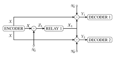
(a) Degraded Gaussian BRC with common relay.

(b) Degraded Gaussian BRC with partial cooperation.

Figure 4: Degraded Gaussian BRCs.

III-C The degraded Gaussian BRC with common relay

Interestingly, the inner and outer bounds in Theorems 9 and 8 coincide for the degraded Gaussian BRC with common relay, as shown in Fig. 4(a). The degraded Gaussian BRC-CR is defined by the outputs:

$$\begin{array}[]{l}Y_{1}=X+X_{1}+\mathpzc{N}_{1},\\ Y_{2}=X+X_{1}+\mathpzc{N}_{2},\\ Z_{1}=X+\tilde{\mathpzc{N}}_{1},\end{array}$$

where the source and the relay have power constraints $P,P_{1}$, and $\mathpzc{N}_{1},\mathpzc{N}_{2},\tilde{\mathpzc{N}}_{1}$ are independent Gaussian noises with variances $N_{1},N_{2},\tilde{N}_{1}$, respectively, such that the noises $\mathpzc{N}_{1},\mathpzc{N}_{2},\tilde{\mathpzc{N}}_{1}$ satisfy the necessary Markov conditions in definition 3. It is enough to assume physical degradedness of the receiver signals respect to the relay, and the stochastic degradedness of one receiver respect to the other one. Indeed, there exist $\mathpzc{N},\mathpzc{N}^{\prime}$ such that:

$$\begin{array}[]{l}\mathpzc{N}_{1}=\tilde{\mathpzc{N}}_{1}+\mathpzc{N},\\ \mathpzc{N}_{2}=\tilde{\mathpzc{N}}_{1}+\mathpzc{N}^{\prime}\end{array}$$

and also ${N}_{1}<{N}_{2}$. The following theorem holds as special case of Theorems 8 and 9.

Theorem 10 (degraded Gaussian BRC-CR)

The capacity region of the degraded Gaussian BRC-CR is

$$\mathcal{C}_{\textrm{BRC-CR}} =\displaystyle{\bigcup\limits_{0\leq\beta,\alpha\leq 1}}\Big{\{}(R_{0}\geq 0,R_{1}\geq 0):\,\,\,$$

$$R_{0} \leq\mathcal{C}\left(\frac{\alpha(P+P_{1}+2\sqrt{\overline{\beta}PP_{1}})}{\overline{\alpha}(P+P_{1}+2\sqrt{\overline{\beta}PP_{1}})+{N}_{2}}\right),$$

$$R_{1} \leq\mathcal{C}\left(\frac{\overline{\alpha}(P+P_{1}+2\sqrt{\overline{\beta}PP_{1}})}{{N}_{1}}\right),$$

$$R_{0}+R_{1} \leq\mathcal{C}\left(\frac{\beta P}{\tilde{N}_{1}}\right)\Big{\}}.$$

We shall not prove this theorem here since it was independently established in [40]. The original inner and outer-bounds initially provided had different forms, but their equivalence was established later using a tuning technique. In our case, these bounds can be simply derived from Theorems 8 and 9. The outer-bound is the same as [40] and the inner bound includes the result in [40]. The equivalence of these bounds can be then established. The inner bound in Theorem 10 is obtained from Theorem 8 by choosing $U$ and $X_{1}$ conditionally independent given $V$. The source divides its power into $\theta P$ and $\overline{\theta}P$ for the first and the second user, respectively. The relay does the same with its power into $\theta_{r}P_{1}$ and $\overline{\theta_{r}}P_{1}$. Then $\gamma$ and $\rho$ represent the correlation coefficient between ($U$,$V$) and ($X_{1}$,$X$), respectively. Parameters $\alpha$ and $\beta$ can be respectively interpreted as the power allocation at the source for both destinations and the correlation coefficient between source and relay signals. The inner bound is calculated by following [40]. The outer-bound remains the same and it equals to the region in Theorem 10, but it is derived in a different way.

III-D Degraded Gaussian BRC with partial cooperation

We next present the capacity region of the Gaussian degraded BRC with partial cooperation, as depicted in Fig. 4(b). In this setting, there is no relay-destination cooperation for the second destination and the first destination is physically degraded respect to the relay signal. Input and output relations are as follows:

$$\begin{array}[]{l}Y_{1}=X+X_{1}+\mathpzc{N}_{1},\\ Y_{2}=X+\mathpzc{N}_{2},\\ Z_{1}=X+\tilde{\mathpzc{N}}_{1}.\end{array}$$

The source and the relay have power constraints $P,P_{1}$, and $\mathpzc{N}_{1},\mathpzc{N}_{2},\tilde{\mathpzc{N}}_{1}$ are independent Gaussian noises with variances $N_{1},N_{2},\tilde{N}_{1}$. In addition to this, there exists $\mathpzc{N}$ such that $\mathpzc{N}_{1}=\tilde{\mathpzc{N}}_{1}+\mathpzc{N}$, which means that $Y_{1}$ is physically degraded respect to $Z_{1}$ and we also assume ${N}_{2}<\tilde{N}_{1}$. The proof of the following theorem is presented in Appendix G.

Theorem 11

(Gaussian degraded BRC with partial cooperation) The capacity region of the Gaussian degraded BRC with partial cooperation is given by

$$\mathcal{C}_{\textrm{BRC-PC}} =\displaystyle{\bigcup\limits_{0\leq\beta,\alpha\leq 1}}\Big{\{}(R_{1}\geq 0,R_{2}\geq 0):$$

$$R_{1} \leq\underset{\beta\in[0,1]}{\max}\min\Big{\{}\mathcal{C}\left(\frac{\displaystyle\alpha\beta P}{\overline{\alpha}P+\widehat{N}_{1}}\right),$$

$$\hskip 14.22636pt\mathcal{C}\left(\displaystyle\frac{\displaystyle\alpha P+{P_{1}}+{2\sqrt{\overline{\beta}\alpha PP_{1}}}}{\overline{\alpha}P+{N}_{1}}\right)\Big{\}},$$

$$R_{2} \leq\mathcal{C}\left(\displaystyle\frac{\displaystyle\overline{\alpha}P}{N_{2}}\right)\Big{\}}.$$

The proof of this theorem is indeed similar to Theorem 7 for the capacity of the semi-degraded BRC. The source assigns power $\alpha P$ to carry the message to destination $Y_{1}$ and $\overline{\alpha}P$ to destination $Y_{2}$. Parameters $\alpha$ and $\beta$ are defined as well as in Theorem 10. Destination $Y_{2}$ is the best receiver so it can decode the message intended for destination $Y_{1}$, even after the help of the relay. It means that both the first relay and the destination appear to be degraded respect to the second destination. So the second destination can correctly decode the interference of other users. However, we emphasize that $Z_{1}$ is not necessarily physically degraded respect to $Y_{2}$, which makes of Theorem 11 a stronger result than that in Theorem 7.

IV Gaussian Simultaneous and Broadcast Relay Channels

In this section, based on the rate regions presented in Section II, we compute achievable rate regions for the Gaussian BRC. The Gaussian BRC is modeled as follows:

$$\begin{array}[]{lcr}\displaystyle Y_{1i}=\frac{X_{i}}{\sqrt{d^{\delta}_{y_{1}}}}+\frac{X_{1i}}{\sqrt{d^{\delta}_{z_{1}y_{1}}}}+\mathpzc{N}_{1i},&&\displaystyle Z_{1i}=\frac{X_{i}}{\sqrt{d^{\delta}_{z_{1}}}}+\tilde{\mathpzc{N}}_{1i},\\ \displaystyle Y_{2i}=\frac{X_{i}}{\sqrt{d^{\delta}_{y_{2}}}}+\frac{X_{2i}}{\sqrt{d^{\delta}_{z_{2}y_{2}}}}+\mathpzc{N}_{2i},&&\displaystyle Z_{2i}=\frac{X_{i}}{\sqrt{d^{\delta}_{z_{2}}}}+\tilde{\mathpzc{N}}_{2i}.\end{array}$$

The channel inputs $\{X_{i}\}$ and the relay inputs $\{X_{1i}\}$ and $\{X_{2i}\}$ must satisfy the power constraints

$$\begin{array}[]{lcr}\displaystyle\sum_{i=1}^{n}X_{i}^{2}\leq nP,&\textrm{and}&\displaystyle\sum_{i=1}^{n}X_{ki}^{2}\leq nP_{k},\,\,\,k=\{1,2\}.\end{array}$$

The channel noises $\tilde{\mathpzc{N}}_{1i},\tilde{\mathpzc{N}}_{2i}$, ${\mathpzc{N}}_{1i},{\mathpzc{N}}_{2i}$ are zero-mean i.i.d. Gaussian RVs of variances $\tilde{{N}}_{1},\tilde{{N}}_{2},N_{1},N_{2}$ and independent of the channel and the relay inputs. The distances $(d_{y_{1}},d_{y_{2}})$ between the source and the destinations $1$ and $2$, respectively, are assumed to be fixed during the communication. Similarly, the distances between the relays and their destinations $(d_{z_{1}y_{1}},d_{z_{2}y_{2}})$. As shown in Fig. 5, notice that in this simultaneous Gaussian relay channel no interference is allowed from the relay $b$ to the destination $\overline{b}=\{1,2\}\setminus\{b\}$, for $b=\{1,2\}$. In the remainder of this section, we evaluate DF-DF, DF-CF and CF-CF regions, and outer-bounds. As for the classical BC, by using superposition coding, we decompose $X$ as the sum of two independent descriptions such that ${\mathbb{E}}\left\{X_{A}^{2}\right\}=\alpha P$ and ${\mathbb{E}}\left\{X_{B}^{2}\right\}=\overline{\alpha}P$, where $\overline{\alpha}=1-\alpha$. The codewords $(X_{A},X_{B})$ contain informations for destinations $Y_{1}$ and $Y_{2}$, respectively.

IV-A DF-DF region for Gaussian BRC

We aim to evaluate the rate region in Theorem 1 for the presented Gaussian BRC. To this end, we rely on well-known coding schemes for broadcast and relay channels. A Dirty-Paper Coding (DPC) scheme is needed for destination $Y_{2}$ to cancel the interference coming from the relay signal $X_{1}$. Similarly, a DPC scheme is needed for destination $Y_{1}$ to cancel the signal noise $X_{B}$ coming from the code of the other user. The auxiliary RVs $(U_{1},U_{2})$ are chosen as:

$$\begin{array}[]{l}U_{1}=X_{A}+\lambda\,\,X_{B}\textrm{ with }\,\,\displaystyle X_{A}=\tilde{X}_{A}+\sqrt{\frac{\overline{\beta_{1}}\alpha P}{P_{1}}}X_{1},\\ U_{2}=X_{B}+\gamma X_{1}\,\,\textrm{ with }\,\,\displaystyle X_{B}=\tilde{X}_{B}+\sqrt{\frac{\overline{\beta_{2}}\overline{\alpha}P}{P_{1}}}X_{2},\end{array}$$

for some parameters $\beta_{1},\beta_{2},\alpha,\gamma,\lambda\in[0,1]$, where the encoder sends $X=X_{A}+X_{B}$. Now choose in Theorem 1 $V_{0}=U_{0}=\emptyset$, $U_{1}=U_{3}$ and $U_{4}=U_{2}$. It can be seen that this choice leads to $I_{M}=0$ and $I_{i}=J_{i}$ for $i=\{1,2\}$. Then for $R_{0}=0$ and based on the above RVs, the next rates are achievable:

$$R_{1}\leq\min\big{\{}I(U_{1};Z_{1}|X_{1}), I(U_{1},X_{1};Y_{1})\big{\}}$$

$$-I(U_{1};X_{2},U_{2}|X_{1}),$$

$$R_{2}\leq\min\big{\{}I(U_{2};Z_{2}|X_{2}), I(U_{2},X_{2};Y_{2})\big{\}}$$

$$-I(X_{1};U_{2}|X_{2}).$$

For destination 1, the achievable rate is the minimum of two mutual informations, where the first term is given by $R_{11}\leq I(U_{1};Z_{1}|X_{1})-I(U_{1};X_{2},U_{2}|X_{1})$. The current problem becomes similar to the conventional DPC with $\tilde{X}_{A}$ as the main message, $X_{B}$ as the interference and $\tilde{N}_{1}$ as the noise. Hence the corresponding rate writes as

$$R_{11}^{(\beta_{1},\lambda)}=$$

$$\frac{1}{2}\log\left[\frac{\displaystyle\alpha\beta_{1}P(\alpha\beta_{1}P+\overline{\alpha}P+d^{\delta}_{z_{1}}\tilde{N}_{1})}{d^{\delta}_{z_{1}}\tilde{N}_{1}(\alpha\beta_{1}P+\lambda^{2}\overline{\alpha}P)+(1-\lambda)^{2}\overline{\alpha}P\alpha{\beta_{1}}P}\right].$$ (3)

The second term is $R_{12}=I(U_{1},X_{1};Y_{1})-I(U_{1};X_{2},U_{2}|X_{1})$, where the first mutual information can be decomposed into two terms $I(X_{1};Y_{1})$ and $I(U_{1};Y_{1}|X_{1})$. Notice that regardless of the former, the rest of the terms in the expression of rate $R_{12}$ are similar to $R_{11}$. The main codeword is $\tilde{X}_{A}$, while $X_{B}$, ${\mathpzc{N}}_{1}$ are the random state and the noise. After adding the term $I(X_{1};Y_{1})$, we obtain

$$R_{12}^{(\beta_{1},\lambda)}=$$

$$\frac{1}{2}\log\left[\frac{\displaystyle\alpha\beta_{1}Pd^{\delta}_{y_{1}}\left(\frac{P}{d^{\delta}_{y_{1}}}+\frac{P_{1}}{d^{\delta}_{z_{1}y_{1}}}+2\sqrt{\frac{\overline{\beta_{1}}\alpha PP_{1}}{d^{\delta}_{y_{1}}d^{\delta}_{z_{1}y_{1}}}}+N_{1}\right)}{\displaystyle d^{\delta}_{y_{1}}{N}_{1}(\alpha\beta_{1}P+\lambda^{2}\overline{\alpha}P)+(1-\lambda)^{2}\overline{\alpha}P\alpha{\beta_{1}}P}\right].$$ (4)

$$R_{21}^{(\beta_{1},\beta_{2},\gamma)}=\frac{1}{2}\log\left[\frac{\displaystyle\overline{\alpha}\beta_{2}P(\overline{\alpha}\beta_{2}P+{\alpha}P+d^{\delta}_{z_{2}}\tilde{N}_{2})}{(d^{\delta}_{z_{2}}\tilde{N}_{2}+\alpha\beta_{1}P)(\overline{\alpha}\beta_{2}P+\gamma^{2}\overline{\beta_{1}}\alpha P)+(1-\gamma)^{2}\overline{\alpha}\beta_{2}P\alpha\overline{\beta_{1}}P}\right],$$ (5)

 

$$R_{22}^{(\beta_{1},\beta_{2},\gamma)}=\frac{1}{2}\log\left[\frac{\displaystyle\overline{\alpha}\beta_{2}Pd^{\delta}_{y_{2}}\left(\frac{P}{d^{\delta}_{y_{2}}}+\frac{P_{2}}{d^{\delta}_{z_{2}y_{2}}}+2\sqrt{\frac{\overline{\beta_{2}}\overline{\alpha}PP_{2}}{d^{\delta}_{y_{2}}d^{\delta}_{z_{2}y_{2}}}}+N_{2}\right)}{(d^{\delta}_{y_{2}}{N}_{2}+\alpha\beta_{1}P)(\overline{\alpha}\beta_{2}P+\gamma^{2}\overline{\beta_{1}}{\alpha}P)+(1-\gamma)^{2}\overline{\alpha}\beta_{2}P\alpha\overline{\beta_{1}}P}\right].$$ (6)

 

Based on expressions (3) and (4), the maximum achievable rate follows as

$$R^{*}_{1}=\underset{0\leq\beta_{1},\lambda\leq 1}{\max}\min\left\{R_{11}^{(\beta_{1},\lambda)},R_{12}^{(\beta_{1},\lambda)}\right\}.$$

For the destinations, the argument is similar to the one above with the difference that for the current DPC, where only $X_{1}$ can be canceled, the rest of $X_{A}$ appears as noise for the destinations. So it becomes the conventional DPC with $\tilde{X}_{B}$ as the main message, $X_{1}$ as the interference, and $\tilde{\mathpzc{N}}_{1}$ and $\tilde{X}_{A}$ as the noises. The rates write as (5) and (6).

And finally the maximum achievable rate follows as

$$R^{*}_{2}=\underset{0\leq\beta_{2},\gamma\leq 1}{\max}\min\left\{R_{21}^{(\beta_{1},\beta_{2},\gamma)},R_{22}^{(\beta_{1},\beta_{2},\gamma)}\right\}.$$

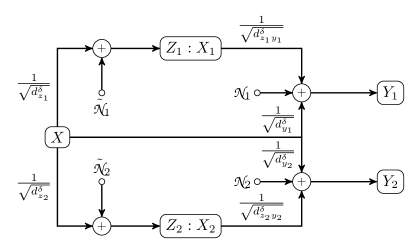
Figure 5: Gaussian BRC

IV-B DF-CF region for the Gaussian BRC

As for the conventional BC, by using superposition coding, we decompose $X=X_{A}+X_{B}$ as a sum of two independent RVs such that ${\mathbb{E}}\left\{X_{A}^{2}\right\}=\alpha P$ and ${\mathbb{E}}\left\{X_{B}^{2}\right\}=\overline{\alpha}P$, where $\overline{\alpha}=1-\alpha$. The codewords $(X_{A},X_{B})$ contain the information intended to receivers $Y_{1}$ and $Y_{2}$, respectively. First, we identify two different cases for which DPC schemes are derived. In the first case, the code is such that the CF destination is able to remove the interference caused by DF code. In the second case, the code is such that DF destination cancels the interference of CF code.

Case I

A DPC scheme is applied to $X_{B}$ to cancel the interference $X_{A}$ while the relay signal is similarly selected to [7]. Hence, the RVs $(U_{1},U_{2})$ are set to

$$U_{1} =X_{A}=\tilde{X}_{A}+\sqrt{\frac{\overline{\beta}\alpha P}{P_{1}}}X_{1},$$ (7)

$$U_{2} =X_{B}+\gamma X_{A},$$ (8)

where $\beta$ is the correlation coefficient between the relay and the source and, $\tilde{X}_{A}$ and $X_{1}$ are independent. Notice that in this case, instead of only $Y_{2}$, we have also $\hat{Z}_{2}$ present which is chosen to as $\hat{Z}_{2}=Z_{2}+\hat{\mathpzc{N}}_{2}$. Thus, DPC should also be able to cancel the interference at both, received and compressed signals having different noise levels. Calculation should be done again with $(Y_{2},\hat{Z}_{2})$, which are the main message $X_{B}$ and the interference $X_{A}$. We can show that the optimum $\gamma$ has a similar form to the classical DPC with the noise term replaced by an equivalent noise which is like the harmonic mean of the noise in $(Y_{2},\hat{Z}_{2})$. The optimum $\gamma^{*}$ is given by

$$\gamma^{*} =\frac{\overline{\alpha}P}{\overline{\alpha}P+N_{t1}},$$

$$N_{t1} =\left[(d^{\delta}_{z_{2}}(\tilde{N}_{2}+\widehat{N}_{2}))^{-1}+(d^{\delta}_{y_{2}}({N}_{2}))^{-1}\right]^{-1}.$$ (9)

As we can see the equivalent noise is twice of the harmonic mean of the other noise terms.

From Corollary 3, we can see that the optimal $\gamma^{*}$ and the current definitions yield the rates

$$R_{1}^{*} =\min\big{\{}I(U_{1};Z_{1}|X_{1}),I(U_{1},X_{1};Y_{1})\big{\}}$$

$$=\underset{0\leq\beta\leq 1}{\max}\min\Big{\{}\mathcal{C}\left(\frac{\alpha\beta P}{\overline{\alpha}P+d^{\delta}_{z_{1}}\tilde{N}_{1}}\right),$$

$$\mathcal{C}\left(\frac{\displaystyle\alpha\frac{P}{d^{\delta}_{y_{1}}}+\frac{P_{1}}{d^{\delta}_{z_{1}y_{1}}}+2\sqrt{\frac{\overline{\beta}\alpha PP_{1}}{d^{\delta}_{y_{1}}d^{\delta}_{z_{1}y_{1}}}}}{\displaystyle\frac{\overline{\alpha}P}{d^{\delta}_{y_{1}}}+{N}_{1}}\right)\Big{\}},$$ (10)

$$R_{2}^{*} =I(U_{2};Y_{2},\hat{Z}_{2}|X_{2})-I(U_{1},X_{1};U_{2})$$ (11)

$$=\mathcal{C}\left(\frac{\overline{\alpha}P}{d^{\delta}_{y_{2}}N_{2}}+\frac{\overline{\alpha}P}{d^{\delta}_{z_{2}}(\widehat{N}_{2}+\tilde{N}_{2})}\right).$$ (12)

Note that since $(X_{A},X_{B})$ are chosen independent, destination 1 sees $X_{B}$ as an additional channel noise. The compression noise is chosen as follows

$$\widehat{N}_{2}={\left(P\left(\frac{1}{d^{\delta}_{y_{2}}N_{2}}+\frac{1}{d^{\delta}_{z_{2}}\tilde{N}_{2}}\right)+1\right)}/{\frac{P_{2}}{d^{\delta}_{y_{2}}N_{2}}}.$$ (13)

Case 2

We use a DPC scheme for destination $Y_{2}$ to cancel the interference $X_{1}$, and next we use a DPC scheme for destination $Y_{1}$ to cancel $X_{B}$. For this case, the auxiliary RVs $(U_{1},U_{2})$ are chosen as

$$\begin{array}[]{l}U_{1}=X_{A}+\lambda\,\,X_{B}\textrm{ with }\,\,X_{A}=\tilde{X}_{A}+\sqrt{\displaystyle\frac{\overline{\beta}\alpha P}{P_{1}}}X_{1},\\ U_{2}=X_{B}+\gamma X_{1}.\end{array}$$ (14)

From Corollary 3, the corresponding rates with the current definitions are

$$R_{1} =\min\big{\{}I(U_{1};Z_{1}|X_{1}),I(U_{1},X_{1};Y_{1})\big{\}}$$

$$\hskip 28.45274pt-I(U_{1};U_{2}|X_{1}),$$ (15)

$$R_{2} =I(U_{2};Y_{2},\hat{Z}_{2}|X_{2})-I(X_{1};U_{2}).$$ (16)

The argument for destination 2 is similar than before but it differs in the DPC. Here only $X_{1}$ can be canceled and then $X_{A}$ remains as additional noise. The optimum $\gamma^{*}$ similar to [50] is given by

$$\gamma^{*} =\sqrt{\frac{\overline{\beta}\alpha P}{P_{1}}}\frac{\overline{\alpha}P}{\overline{\alpha}P+N_{t2}},$$ (17)

$$N_{t2} =\big{(}(d^{\delta}_{z_{2}}(\tilde{N}_{2}+\widehat{N}_{2})$$

$$\hskip 28.45274pt+{\beta}\alpha P)^{-1}+(d^{\delta}_{y_{2}}({N}_{2})+{\beta}\alpha P)^{-1}\big{)}^{-1},$$ (18)

and

$$R_{2}^{*}=\mathcal{C}\left(\frac{\overline{\alpha}P}{d^{\delta}_{y_{2}}N_{2}+{\beta}\alpha P}+\frac{\overline{\alpha}P}{d^{\delta}_{z_{2}}(\widehat{N}_{2}+\tilde{N}_{2})+{\beta}\alpha P}\right).$$ (19)

For destination 1, the achievable rate is the minimum of two terms, where the first one is given by

$$R_{11}^{(\beta,\lambda)}=I(U_{1};Z_{1}|X_{1})-I(U_{1};U_{2}|X_{1})$$

$$=\frac{1}{2}\log\left(\frac{\alpha\beta P(\alpha\beta P+\overline{\alpha}P+d^{\delta}_{z_{1}}\tilde{N}_{1})}{d^{\delta}_{z_{1}}\tilde{N}_{1}(\alpha\beta P+\lambda^{2}\overline{\alpha}P)+(1-\lambda)^{2}\overline{\alpha}P\alpha{\beta}P}\right).$$ (20)

The second term is $R_{12}=I(U_{1}X_{1};Y_{1})-I(U_{1};U_{2}|X_{1})$, where the first mutual information can be decomposed into two terms $I(X_{1};Y_{1})$ and $I(U_{1};Y_{1}|X_{1})$. Notice that regardless of the former, the rest of the terms in the expression of the rate $R_{12}$ are similar to $R_{11}$. The main codeword is $\tilde{X}_{A}$, while $X_{B}$ and ${\mathpzc{N}}_{1}$ represent the random state and the noise, respectively. After adding the term $I(X_{1};Y_{1})$, we obtain

$$R_{12}^{(\beta,\lambda)}=$$

$$\frac{1}{2}\log\left[\frac{\displaystyle\alpha\beta Pd^{\delta}_{y_{1}}\left(\frac{P}{d^{\delta}_{y_{1}}}+\frac{P_{1}}{d^{\delta}_{z_{1}y_{1}}}+2\sqrt{\frac{\overline{\beta}\alpha PP_{1}}{d^{\delta}_{y_{1}}d^{\delta}_{z_{1}y_{1}}}}+N_{1}\right)}{{N}_{1}d^{\delta}_{y_{1}}(\alpha\beta P+\lambda^{2}\overline{\alpha}P)+(1-\lambda)^{2}\overline{\alpha}P\alpha{\beta}P}\right].$$ (21)

Based on expressions (21) and (20), the maximum achievable rate follows as

$$R^{*}_{1}=\underset{0\leq\beta,\lambda\leq 1}{\max}\min\big{\{}R_{11}^{(\beta,\lambda)},R_{12}^{(\beta,\lambda)}\big{\}}.$$ (22)

It should be noted that the constraint for $\widehat{N}_{2}$ is still the same as (13).

IV-C CF-CF region for the Gaussian BRC

We now investigate the Gaussian BRC for the CF-CF region, where the relays are collocated with the destinations. In this setting, the compression noises are chosen as follows:

$$\hat{Z}_{1} =Z_{1}+\hat{\mathpzc{N}}_{1},$$

$$\hat{Z}_{2} =Z_{2}+\hat{\mathpzc{N}}_{2},$$ (23)

where $\hat{\mathpzc{N}}_{1},\hat{\mathpzc{N}}_{2}$ are zero-mean Gaussian noises of variances $\hat{N}_{1},\hat{N}_{2}$. As for the conventional BC, by using superposition coding, we decompose $X=X_{A}+X_{B}$ as a sum of two independent RVs such that ${\mathbb{E}}\left\{X_{A}^{2}\right\}=\alpha P$ and ${\mathbb{E}}\left\{X_{B}^{2}\right\}=\overline{\alpha}P$, where $\overline{\alpha}=1-\alpha$. The codewords $(X_{A},X_{B})$ contain the information intended to destinations $Y_{1}$ and $Y_{2}$. A DPC scheme is applied to $X_{B}$ to cancel interference $X_{A}$ while the relay signal is similarly selected to [7]. So the auxiliary RVs $(U_{1},U_{2})$ are set to

$$U_{1}=X_{A},\,\,\,\,U_{2}=X_{B}+\gamma X_{A}.$$ (24)

Notice that, in this case, instead of only $Y_{2}$ we have also $\hat{Z}_{2}$ present in the rate. Thus, DPC should be also able to cancel the interference in both, received and compressed signals which have different noise levels. Calculation should be done again with $(Y_{2},\hat{Z}_{2})$ which are the main message $X_{B}$ and the interference $X_{A}$. It can be shown that the optimum $\gamma$ has a similar form to the classical DPC with the noise term replaced by an equivalent noise which is like the harmonic mean of the noises in $(Y_{2},\hat{Z}_{2})$. The optimum

$$\gamma^{*} =\frac{\overline{\alpha}P}{\overline{\alpha}P+N_{t1}},$$

$$N_{t1} =\left[1/(d^{\delta}_{z_{2}}(\tilde{N}_{2}+\widehat{N}_{2}))+1/(d^{\delta}_{y_{2}}{N}_{2})\right]^{-1}.$$ (25)

Observe that the equivalent noise is twice of the harmonic mean of the other noise terms. We use Theorem 3 with $U_{0}=\phi$ to find the following rates

$$R_{1}^{*} =I(U_{1};Y_{1},\hat{Z}_{1}|X_{1})$$

$$=\mathcal{C}\left(\frac{{\alpha}P}{d^{\delta}_{y_{1}}N_{1}+\overline{\alpha}P}+\frac{{\alpha}P}{d^{\delta}_{z_{1}}(\widehat{N}_{1}+\tilde{N}_{1})+\overline{\alpha}P}\right),$$

$$R_{2}^{*} =I(U_{2};Y_{2},\hat{Z}_{2}|X_{2})-I(U_{1}X_{1};U_{2})$$ (26)

$$=\mathcal{C}\left(\frac{\overline{\alpha}P}{d^{\delta}_{y_{2}}N_{2}}+\frac{\overline{\alpha}P}{d^{\delta}_{z_{2}}(\widehat{N}_{2}+\tilde{N}_{2})}\right).$$ (27)

Note that since $(X_{A},X_{B})$ are chosen independent, destination 1 sees $X_{B}$ as additional channel noise. The compression noises are chosen as follows:

$$\hat{N}_{1}=\tilde{N}_{1}{\left[P\left(\frac{1}{d^{\delta}_{y_{1}}N_{1}}+\frac{1}{d^{\delta}_{z_{1}}\tilde{N}_{1}}\right)+1\right]}/{\frac{P_{1}}{d^{\delta}_{z_{1}y_{1}}N_{1}}},$$

$$\hat{N}_{2}=\tilde{N}_{2}{\left[P\left(\frac{1}{d^{\delta}_{y_{2}}N_{2}}+\frac{1}{d^{\delta}_{z_{2}}\tilde{N}_{2}}\right)+1\right]}/{\frac{P_{2}}{d^{\delta}_{z_{2}y_{2}}N_{2}}}.$$ (28)

Common-rate

The goal is to send common-information at rate $R_{0}$. To this end, define $X=U_{0}$ and evaluate Theorem 3 with $U_{1}=U_{2}=\phi$. It is easy to verify that the following common-rate is achievable

$$R_{0}\leq\min\Big{\{} \mathcal{C}\left(\frac{P}{d^{\delta}_{y_{1}}N_{1}}+\frac{P}{d^{\delta}_{z_{1}}(\widehat{N}_{1}+\tilde{N}_{1})}\right),$$

$$\mathcal{C}\left(\frac{P}{d^{\delta}_{y_{2}}N_{2}}+\frac{P}{d^{\delta}_{z_{2}}(\widehat{N}_{2}+\tilde{N}_{2})}\right)\Big{\}}.$$ (29)

The constraints for compression noises remain the same as before.

IV-D The source is oblivious to the cooperative strategy adopted by the relay

In this setting, we deal with two different models referred to as the Compound relay channel (RC) and the Composite relay channel (RC).

IV-D1 Compound RC

The goal is to send common-information at rate $R_{0}$ based on the DF-CF region. The definition of the channels remain the same. We set $X=U+\sqrt{\displaystyle\frac{\overline{\beta}P}{P_{1}}}X_{1}$ and evaluate Corollary 2. It is easy to verify that the achievable rate $R_{\textrm{DF}}$ for the destination $Y_{1}$ writes as

$$R_{\textrm{DF}}\leq \min\Big{\{}\mathcal{C}\left(\frac{\beta P}{d^{\delta}_{z_{1}}\tilde{N}_{1}}\right),$$

$$\mathcal{C}\left(\frac{\displaystyle\frac{P}{d^{\delta}_{y_{1}}}+\frac{P_{1}}{\displaystyle d^{\delta}_{z_{1}y_{1}}}+2\sqrt{\displaystyle\frac{\displaystyle\overline{\beta}PP_{1}}{d^{\delta}_{y_{1}}d^{\delta}_{z_{1}y_{1}}}}}{{N}_{1}}\right)\Big{\}}.$$ (30)

For destination $Y_{2}$, the CF rate $I(X;Y_{2},\hat{Z}_{2}|X_{2})$ is as follows

$$R_{\textrm{CF}}\leq\mathcal{C}\left(\frac{P}{d^{\delta}_{y_{2}}N_{2}}+\frac{P}{d^{\delta}_{z_{2}}(\widehat{N}_{2}+\tilde{N}_{2})}\right).$$ (31)

The upper bound from Theorem 6 writes as the next rate

$$C\leq\underset{0\leq\beta_{1},\beta_{2}\leq 1}{\max}\min \Big{\{}\mathcal{C}\left(\displaystyle\beta_{1}P\left[\frac{1}{\displaystyle d^{\delta}_{z_{1}}\tilde{N}_{1}}+\frac{1}{\displaystyle d^{\delta}_{y_{1}}{N}_{1}}\right]\right),$$

$$\mathcal{C}\left(\displaystyle\frac{\displaystyle\frac{P}{\displaystyle d^{\delta}_{y_{1}}}+\displaystyle\frac{P_{1}}{d^{\delta}_{z_{1}y_{1}}}+2\sqrt{\frac{\displaystyle\overline{\beta}_{1}PP_{1}}{d^{\delta}_{y_{1}}d^{\delta}_{z_{1}y_{1}}}}}{{N}_{1}}\right),$$

$$\mathcal{C}\left(\beta_{2}P\left[\frac{1}{d^{\delta}_{z_{2}}\tilde{N}_{2}}+\frac{1}{d^{\delta}_{y_{2}}{N}_{2}}\right]\right),$$

$$\mathcal{C}\left(\frac{\displaystyle\frac{P}{d^{\delta}_{y_{2}}}+\frac{P_{2}}{d^{\delta}_{z_{2}y_{2}}}+2\sqrt{\displaystyle\frac{\displaystyle\overline{\beta}_{2}PP_{2}}{\displaystyle d^{\delta}_{y_{2}}d^{\delta}_{z_{2}y_{2}}}}}{{N}_{2}}\right)\Big{\}}.$$ (32)

Observe that the rate (31) is exactly the same as the Gaussian CF rate [15]. This means that DF based on regular encoding can be also decoded with the CF strategy, as well as the case with collocated relay and receiver [74]. By using the proposed coding, it is possible to send common information at the minimum rate between DF (30) and CF (31) rates

$$R_{0}=\min\{R_{\textrm{DF}},R_{\textrm{CF}}\}.$$

For the case of private information, we have shown that any pair of rates $(R_{\textrm{DF}}\leq R^{*}_{1},R_{\textrm{CF}}\leq R^{*}_{2})$ given by (19) and (22) are admissible and thus $(R_{\textrm{DF}},R_{\textrm{CF}})$ can be simultaneously sent.

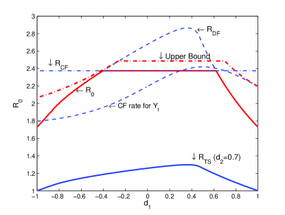
Figure 6: Common-rate of the Gaussian BRC with DF-CF strategies.

Fig. 6 shows numerical evaluation of the common-rate $R_{0}$. All channel noises are set to the unit variance and $P=P_{1}=P_{2}=10$. The distance between $X$ and $(Y_{1},Y_{2})$ is one while $d_{z_{1}}=d_{1}$, $d_{z_{1}y_{1}}=1-d_{1}$, $d_{z_{2}}=d_{2}$, $d_{z_{2}y_{2}}=1-d_{2}$. Relay 1 moves with $d_{1}\in\left[-1,1\right]$ and Fig. 6 presents rates as a function of $d_{1}$. Whereas the position of relay 2 is assumed to be fixed to $d_{2}=0.7$ so $R_{\textrm{CF}}$ is a constant function of $d_{1}$, but $R_{\textrm{DF}}$ depends on $d_{1}$. For comparison, CF rate for destination $Y_{1}$ is also plotted which corresponds to the case where the first relay uses CF scheme. This setting serves to compare the performances of coding respect to the relay position. We remark that one can achieve the minimum between CF and DF rates. These rates are also compared with a naive time-sharing strategy which consists on DF scheme $\tau\%$ of time and CF scheme $(1-\tau)\%$ of time. Time-sharing yields the following achievable rate

$$R_{\textrm{TS}}=\underset{0\leq\tau\leq 1}{\max}\min\{\tau R_{\textrm{DF}},(1-\tau)R_{\textrm{CF}}\}.$$

Notice that with the proposed coding scheme significant gains can be achieved when the relay is close to the source, i.e., DF scheme is more suitable, compared to the worst case.

IV-D2 Composite RC

Consider now a composite model where the relay is collocated with the source with probability $p$ (refer to it as the first channel) and with the destination with probability $1-p$ (refer to it as the second channel). Therefore, DF scheme is the suitable strategy for the first channel while CF scheme performs better on the second one. Define the expected rate as

$$R_{av}=R_{0}+pR_{1}+(1-p)R_{2},$$

for any achievable triple of rates $(R_{0},R_{1},R_{2})$. Expected rate based on the proposed coding strategy is compared to conventional strategies. Alternative coding schemes for this scenario, where the encoder can simply invest on one coding scheme DF or CF, are possible. In fact, there are different ways to proceed:

• Send information via DF scheme at the best possible rate between both channels. Then the worst channel cannot decode and thus the expected rate becomes $p^{\max}_{\textrm{DF}}R^{\max}_{\textrm{DF}}$, where $R^{\max}_{\textrm{DF}}$ is the DF rate achieved on the best channel and $p^{\max}_{\textrm{DF}}$ is its probability.

• Send information via the DF scheme at the rate of the worst (second) channel and hence both users can decode the information at rate $R^{\min}_{\textrm{DF}}$. Finally the next expected rate is achievable by investing on only one coding scheme

  $$R_{av}^{\textrm{DF}}=\max\big{\{}p^{\max}_{\textrm{DF}}R^{\max}_{\textrm{DF}},R^{\min}_{\textrm{DF}}\big{\}}.$$

• By investing on CF scheme with the same arguments as before, the expected rate writes as

  $$R_{av}^{\textrm{CF}}=\max\big{\{}p^{\max}_{\textrm{CF}}R^{\max}_{\textrm{CF}},R^{\min}_{\textrm{CF}}\big{\}},$$

  with definitions of $(R^{\min}_{\textrm{CF}},R^{\max}_{\textrm{CF}},p^{\max}_{\textrm{CF}})$ similar to before.

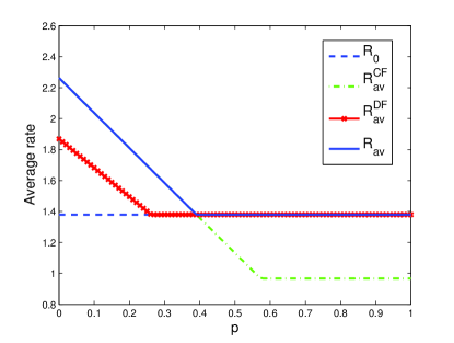
Figure 7: Expected rate for the composite Gaussian relay channel.

Fig. 7 shows numerical evaluation of the average rate. All channel noises are set to have unit variance and $P=P_{1}=P_{2}=10$. The distance between $X$ and $(Y_{1},Y_{2})$ is $(3,1)$, while $d_{z_{1}}=1$, $d_{z_{1}y_{1}}=2$, $d_{z_{2}}=0.9$, $d_{z_{2}y_{2}}=0.1$. As one can see, the common-rate strategy provides a fixed rate all time which is always better than the worst case. However, at one corner full investment on one rate performs better because the high probability of one channel reduces the effect of the other. Based on the proposed coding scheme, i.e., using common and private messages, it is possible to cover all corner points performing better than both full investment strategies. It is worth to mention that the corner zone only requires private information of one channel.

IV-E The source is oblivious to the presence of relay

We now focus on a scenario where the source is unaware of the relay’s presence. This arises, for example, when the informed relay decides by itself to help the destination whenever relaying is efficient (e.g. channel conditions are good enough). In this case, the BRC would have a single relay node. It is assumed here that there is no common information, then we set $X_{2}=\emptyset$ and $Z_{2}=Y_{2}$. The Gaussian BRC is defined as follows:

$$Y_{1} = X+X_{1}+\mathpzc{N}_{1},$$

$$Y_{2} = X+\mathpzc{N}_{2},$$

$$Z_{1} = X+\widehat{\mathpzc{N}}_{1}.$$ (33)

As for the classical BC, by using superposition coding, we decompose $X$ as the sum of two independent descriptions such that ${\mathbb{E}}\left\{X_{A}^{2}\right\}=\alpha P$ and ${\mathbb{E}}\left\{X_{B}^{2}\right\}=\overline{\alpha}P$, where $\overline{\alpha}=1-\alpha$. The codewords $(X_{A},X_{B})$ contain the information intended for destinations $Y_{1}$ and $Y_{2}$, respectively. We use a DPC scheme applied to $X_{B}$ to cancel the interference $X_{A}$ while the relay signal is similarly chosen as in [7]. Hence, the auxiliary RVs $(U_{1},U_{2})$ are set to

$$\begin{array}[]{l}U_{1}=X_{A}=\tilde{X}_{A}+\sqrt{\displaystyle\frac{\overline{\beta}\alpha P}{P_{1}}}X_{1},\\ U_{2}=X_{B}+\gamma X_{A},\end{array}$$ (34)

where $\beta$ is the correlation coefficient between relay and source signals, and $\tilde{X}_{A}$ and $X_{1}$ are independent.

The distance between the relay and the source is denoted by $d_{1}$, between the relay and destination 1 by $1-d_{1}$ and between destination 2 and the source by $d_{2}$. The new Gaussian BRC writes as: $Z_{1}={X}/{d_{1}}+\widehat{\mathpzc{N}}_{1}$, $Y_{1}=X+{X_{1}}/{(1-d_{1})}+\mathpzc{N}_{1}$ and $Y_{2}={X}/{d_{2}}+\mathpzc{N}_{2}$. From the previous section, the achievable rates are

$$R_{1}^{*} =\underset{\beta\in[0,1]}{\max}\min\Big{\{}\mathcal{C}\left(\frac{\displaystyle\alpha\beta P}{\overline{\alpha}P+d^{2}_{1}\widehat{N}_{1}}\right),$$

$$\hskip 28.45274pt\mathcal{C}\left(\displaystyle\frac{\displaystyle\alpha P+\frac{P_{1}}{(1-d_{1})^{2}}+\frac{2\sqrt{\overline{\beta}\alpha PP_{1}}}{|1-d_{1}|}}{\overline{\alpha}P+{N}_{1}}\right)\Big{\}},$$

$$R_{2}^{*} =\mathcal{C}\left(\displaystyle\frac{\displaystyle\overline{\alpha}P}{d^{2}_{2}N_{2}}\right).$$ (35)

Notice that since $(X_{A},X_{B})$ are independent then destination 1 sees $X_{B}$ as additional noise. The following outer-bound can be also derived for this channel:

$$R_{1} \leq\underset{\beta\in[0,1]}{\max}\min\Big{\{}\mathcal{C}\left(\frac{\displaystyle\alpha\beta P}{\overline{\alpha}P+d^{2}_{1}\widehat{N}_{1}}+\frac{\displaystyle\alpha\beta P}{\overline{\alpha}P+{N}_{1}}\right),$$

$$\hskip 28.45274pt\mathcal{C}\left(\displaystyle\frac{\displaystyle\alpha P+\frac{P_{1}}{(1-d_{1})^{2}}+\frac{2\sqrt{\overline{\beta}\alpha PP_{1}}}{|1-d_{1}|}}{\overline{\alpha}P+{N}_{1}}\right)\Big{\}},$$

$$R_{2} \leq\mathcal{C}\left(\displaystyle\frac{\displaystyle\overline{\alpha}P}{d^{2}_{2}N_{2}}\right).$$ (36)

Note that if the relay channel is degraded, the bound in (36) reduces to the rate region in (35) and thus we have the capacity of this channel according to Theorem 11. It can be seen that the broadcast strategy provides significant gains compare to the simple time-sharing scheme which consists in sharing over time the information for both destinations.

V Summary and Discussion

In this paper we investigated cooperative strategies for simultaneous and broadcast relay channels. Several cooperative schemes have been proposed and the corresponding inner and outer-bounds on the capacity region were derived. The focus was on the simultaneous relay channel (SRC) with two relay channels, where the central idea is this problem can be turned into the broadcast relay channel (BRC). Then each branch of this new channel represents one of the possible relay channels. In this setting, the source wishes to send common information to guarantee a minimum amount of information regardless of the channel and additional private information to each of the destinations.

Depending on the nature of the channels involved, it is well-known that the best way to cover the information from the relays tothe destinations is not the same. Based on the best known cooperative strategies, namely, Decode-and-Forward (DF) and Compress-and-Forward (CF), achievable rate regions for three different scenarios of interest have been derived. These are summarized as follows: (i) both relay nodes use DF scheme, (ii) one relay uses CF scheme while the other uses DF scheme, and (iii) both relay nodes use CF scheme. In particular, for region (ii) it is shown that superposition coding can work with CF scheme without incurring performance losses. These inner bounds are shown to be tight for some specific scenarios, yielding capacity results for the semi-degraded BRC with common relay (BRC-CR) and two classes of Gaussian degraded BRC-CRs. Whereas the bounds seem to be not tight for the general degraded BRC-CR. An outer-bound on the capacity of the general BRC was also derived. One should emphasize that when the relays are not present this bound reduces to the best known outer-bound for general broadcast channels (referred to as $UVW$-outer-bound). Similarly, when only one relay channel is present at once this bound reduces to the cut-set bound for the general relay channel.

Finally, application examples for Gaussian channels have been studied and achievable rates were computed for all inner bounds. Special attention was given to two models of practical importance for opportunistic and oblivious cooperation in wireless networks. The first model refers to the situation where the source must be oblivious to the cooperative strategy adopted by the relay (e.g. DF or CF scheme). The second one models the situation where the source must be oblivious to the presence of a nearby relay which may help the communication between source and destination. Numerical results evaluate the gains that can be achieved with the proposed coding strategies compared to naive approaches.

As future work, it would be interesting to exploit these results in the context of composite relay networks with random parameters (e.g. fading, spatial position of nodes, etc.) where performance is measured in terms of capacity versus outage notions. Of particular interest is the investigation of novel rate regions based on (linear) structured coding, e.g., lattice codes [14], which in some cases can improve on random coding.

Appendix A Sketch of Proof of Theorem 1

To prove the theorem, first split the private information $W_{b}$ into non-negative indices $(S_{0b},S_{b},S_{b+2})$ with $b=\{1,2\}$. Then, merge the common information $W_{0}$ with a part of private information $(S_{01},S_{02})$ into a single message, as shown in Fig. 3(b). Hence we obtain that $R_{b}=S_{b+2}+S_{b}+S_{0b}$. For notation simplicity, we denote $\underline{u}=u_{1}^{n}$ for every $u$. We now consider the main steps for codebook generation, encoding and decoding procedures.
Code generation:

1. Generate $2^{nT_{0}}$ i.i.d. sequences $\underline{v}_{0}$ each with PD

   $$P_{V_{0}}(\underline{v}_{0})=\prod_{j=1}^{n}p_{V_{0}}(v_{0j}),$$

   and index them as $\underline{v}_{0}(r_{0})$ with $r_{0}=\left[1:2^{nT_{0}}\right]$.

2. For each $\underline{v}_{0}(r_{0})$, generate $2^{nT_{0}}$ i.i.d. sequences $\underline{u}_{0}$ each with PD

   $$P_{U_{0}|V_{0}}(\underline{u}_{0}|\underline{v}_{0}(r_{0}))=\prod_{j=1}^{n}p_{U_{0}|V_{0}}(u_{0j}|v_{0j}(r_{0})),$$

   and index them as $\underline{u}_{0}(r_{0},t_{0})$ with $t_{0}=\left[1:2^{nT_{0}}\right]$.

3. For $b\in\{1,2\}$ and each $\underline{v}_{0}(r_{0})$, generate $2^{nT_{b}}$ i.i.d. sequences $\underline{x}_{b}$ each with PD

   $$P_{X_{b}|V_{0}}(\underline{x}_{b}|\underline{v}_{0}(r_{0}))=\prod_{j=1}^{n}p_{X_{b}|V_{0}}(x_{bj}|v_{0j}(r_{0})),$$

   and index them as $\underline{x}_{b}(r_{0},r_{b})$ with $r_{b}=\left[1:2^{nT_{b}}\right]$.

4. Partition the set $\big{\{}1,\dots,2^{nT_{0}}\big{\}}$ into $2^{n(R_{0}+S_{01}+S_{02})}$ cells (similarly to [62]) and label them as $S_{w_{0},s_{01},s_{02}}$. In each cell there are $2^{n(T_{0}-R_{0}-S_{01}-S_{02})}$ elements.

5. For each $b=\{1,2\}$ and every pair $\big{(}\underline{u}_{0}(r_{0},t_{0}),$ $\underline{x}_{b}(r_{0},r_{b})\big{)}$ chosen in the bin $(w_{0},s_{01},s_{02})$, generate $2^{nT_{b}}$ i.i.d. sequences $\underline{u}_{b}$ each with PD

   $$P_{U_{b}|U_{0}X_{b}V_{0}}\big{(}\underline{u}_{b}|\underline{u}_{0}(r_{0},t_{0}),\underline{x}_{b}(r_{0},r_{b}),\underline{v}_{0}(r_{0})\big{)}=$$

   $$\prod_{j=1}^{n}p_{U_{b}|U_{0}X_{b}V_{0}}(u_{bj}|u_{0j}(r_{0},t_{0}),x_{bj}(r_{0},r_{b}),v_{0j}(r_{0})),$$

   and index them as $\underline{u}_{b}(r_{0},t_{0},r_{b},t_{b})$ with $t_{b}=\left[1:2^{nT_{b}}\right]$.

6. For $b=\{1,2\}$, partition the set $\big{\{}1,\ldots,2^{nT_{b}}\big{\}}$ into $2^{nS_{b}}$ cells and label them as $S_{s_{b}}$. In each cell there are $2^{n(T_{b}-S_{b})}$ elements.

7. For each $b=\{1,2\}$ and every pair of sequences $\big{(}\underline{u}_{1}(r_{0},t_{0},r_{1},t_{1}),$ $\underline{u}_{2}(r_{0},t_{0},r_{2},t_{2})\big{)}$ chosen in the bin $(s_{1},s_{2})$, generate $2^{nT_{b+2}}$ i.i.d. sequences $\underline{u}_{b+2}$ each with PD

   $$P_{U_{b+2}|U_{b}}( \underline{u}_{b+2}|\underline{u}_{b}(r_{0},t_{0},r_{b},t_{b}))=$$

   $$\prod_{j=1}^{n}p_{U_{b+2}|U_{b}}(u_{(b+2)j}|u_{bj}(r_{0},t_{0},r_{b},t_{b})).$$

   Index them as $\underline{u}_{b+2}(r_{0},t_{0},r_{b},t_{b},t_{b+2})$ with $t_{b+2}\in\left[1,2^{nT_{b+2}}\right]$.

8. For $b=\{1,2\}$, partition the set $\big{\{}1,\ldots,2^{nT_{b+2}}\big{\}}$ into $2^{nS_{b+2}}$ cells and label them as $S_{s_{b+2}}$. In each cell there are $2^{n(T_{b+2}-S_{b+2})}$ elements.

9. Finally, use a deterministic function for generating $\underline{x}$ as $f\left(\underline{u}_{3},\underline{u}_{4}\right)$ indexed by
   $\underline{x}(r_{0},t_{0},r_{1},r_{2},t_{1},t_{2},t_{3},t_{4})$.

Encoding Part: Transmission is done over $B+1$ block where the encoding in block $i$ is as follows:

1. First, reorganize the current message $(w_{0i},w_{1i},w_{2i})$ into $(w_{0i},s_{01i},s_{02i},s_{1i},s_{2i},s_{3i},s_{4i})$.

2. Then for each $b=\{1,2\}$, relay $b$ already knows about the index $(t_{0(i-1)},t_{b(i-1)})$, so it sends $\underline{x}_{b}\big{(}t_{0(i-1)},t_{b(i-1)}\big{)}$.

3. For each $\underline{v}_{0}(t_{0(i-1)})$, the encoder searches for an index $t_{0i}$ at the cell $S_{w_{0i},s_{01i},s_{02i}}$ such that $\underline{u}_{0}\big{(}t_{0(i-1)},t_{0i}\big{)}$ is jointly typical with $\big{(}\underline{x}_{1}(t_{0(i-1)},t_{1(i-1)}),\underline{x}_{2}(t_{0(i-1)},t_{2(i-1)}),\underline{v}_{0}(t_{0(i-1)})\big{)}$. The success of this step requires that [62]

   $$T_{0}-R_{0}-S_{01}-S_{02}\geq I(U_{0};X_{1},X_{2}|V_{0}).$$ (37)

4. For each $b=\{1,2\}$ and every cell $S_{s_{bi}}$, define $\mathcal{L}_{b}$ as the set of all sequences $\underline{u}_{b}\big{(}t_{0(i-1)},t_{0i},t_{b(i-1)},t_{bi}\big{)}$ for $t_{bi}\in{S}_{s_{bi}}$ which are jointly typical with

   $$\big{(}\underline{x}_{\overline{b}}(t_{0(i-1)}, t_{\overline{b}(i-1)}),\underline{v}_{0}(t_{0(i-1)}),$$

   $$\underline{u}_{0}(t_{0(i-1)},t_{0i}),\underline{x}_{b}(t_{0(i-1)},t_{b(i-1)})\big{)}$$

   where $\overline{b}=\{1,2\}\setminus\{b\}$. In order to create $\mathcal{L}_{b}$, we look for the $\underline{u}_{b}$-index inside the cell $S_{s_{bi}}$ and find $\underline{u}_{b}$ such that it belongs to the set of $\epsilon$-typical $n$-sequences $\textsl{A}^{n}_{\epsilon}(V_{0}U_{0}X_{1}X_{2}U_{b})$.

5. Look for a pair $(\underline{u}_{1}\in\mathcal{L}_{1},\underline{u}_{2}\in\mathcal{L}_{2})$ such that $\big{(}\underline{u}_{1}(t_{0(i-1)},t_{0i},t_{1(i-1)},t_{1i}),\underline{u}_{2}(t_{0(i-1)},t_{0i},t_{2(i-1)},t_{2i})\big{)}$ are jointly typical given the RVs $\big{(}\underline{v}_{0}(t_{0(i-1)}),\underline{x}_{2}(t_{0(i-1)},t_{2(i-1)}),$ $\underline{x}_{1}(t_{0(i-1)},t_{1(i-1)}),\underline{u}_{0}(t_{0(i-1)},t_{0i})\big{)}$. The success of coding steps (iv) and (v) requires

   $$T_{b}-S_{b} \geq I(U_{b};X_{\overline{b}}|X_{b},U_{0},V_{0}),$$

   $$T_{1}+T_{2}-S_{1}-S_{2} \geq I(U_{1};X_{2}|X_{1},U_{0},V_{0})$$

   $$+I(U_{2};X_{1}|X_{2},U_{0},V_{0})$$

   $$+I(U_{2};U_{1}|X_{1},X_{2},U_{0},V_{0}).$$ (38)

   Notice that the first inequality in the above expression, for $b=\{1,2\}$, guarantees the existence of non-empty sets $(\mathcal{L}_{1},\mathcal{L}_{2})$, and the last one is for the step (iv).

6. The encoder searches for indices $t_{3i}\in S_{s_{3i}}$ and $t_{4i}\in S_{s_{4i}}$ such that $\underline{u}_{3}\big{(}t_{0(i-1)},t_{0i},t_{1(i-1)},t_{1i},t_{3i}\big{)}$ and $\underline{u}_{4}\big{(}t_{0(i-1)},t_{0i},t_{2(i-1)},t_{2i},t_{4i}\big{)}$ are jointly typical given each typical pair of $\underline{u}_{1}(t_{0(i-1)},t_{0i},t_{1(i-1)},t_{1i})$ and $\underline{u}_{2}(t_{0(i-1)},t_{0i},t_{2(i-1)},t_{2i})$. The success of this encoding step requires

   $$\!\!\!\!\!\!\!\!T_{3}+T_{4}-S_{3}-S_{4}\geq I(U_{3};U_{4}|U_{1},U_{2},X_{1},X_{2},U_{0},V_{0}).$$ (39)

7. Once the encoder found $(t_{0i},t_{1i},t_{2i},t_{3i},t_{4i})$ (based on the code generation) corresponding to $(w_{0i},\\ s_{01i},s_{02i},s_{1i},s_{2i},s_{3i},s_{4i})$, it transmits $\underline{x}(r_{0(i-1)},t_{0i},r_{1(i-1)},r_{2(i-1)},t_{1i},t_{2i},t_{3i},t_{4i})$. $t_{0i}$ carries the common message after bit recombination and Marton coding. The indices $t_{1i},t_{3i}$ and $t_{2i},t_{4i}$ are, respectively, private information for destinations $Y_{1}$ and $Y_{2}$. Whereas indices $t_{3i}$ and $t_{4i}$, corresponding to partial encoding, are directly transmitted to the intended destinations.

Decoding Part: In block $i$, in order to decode messages relays assume that all messages up to block $i-1$ have been correctly decoded and then decode the current messages in the same block. The destinations use backward decoding and assume that all messages until block $i+1$ have been correctly decoded.

1. First for $b=\{1,2\}$, the relay $b$ after receiving $\underline{z}_{bi}$ tries to decode $(t_{0i},t_{bi})$. The relay is aware of $(V_{0},X_{b})$ because it is supposed to know about $(t_{0(i-1)},t_{b(i-1)})$. The relay $b$ declares that the pair $(t_{0i},t_{bi})$ is sent if the following conditions are simultaneously satisfied:

   1. $\underline{u}_{0}(t_{0(i-1)},t_{0i})$ is jointly typical with $\big{(}\underline{z}_{bi}$, $\underline{v}_{0}(t_{0(i-1)}),$ $\underline{x}_{b}(t_{0(i-1)},t_{b(i-1)})\big{)}$.

   2. $\underline{u}_{b}(t_{0(i-1)},t_{0i},t_{b(i-1)},t_{bi})$ is jointly typical with $\big{(}\underline{z}_{bi}$, $\underline{v}_{0}(t_{0(i-1)}),$ $\underline{x}_{b}(t_{0(i-1)},t_{b(i-1)})\big{)}$.

   Notice that $\underline{u}_{0}$ has been generated independent of $\underline{x}_{b}$ and hence $\underline{x}_{b}$ does not appear in the given part of mutual information. This is an important issue that may increase the region. Constraints for reliable decoding are:

   $$T_{b} <I(U_{b};Z_{b}|U_{0},V_{0},X_{b}),$$ (40)

   $$\!\!\!\!T_{b}+T_{0} <I(U_{b};Z_{b}|U_{0},V_{0},X_{b})+I(U_{0};Z_{b},X_{b}|V_{0}).\!\!\!\!$$ (41)

   Remark 10

   The intuition behind expressions (40) and (41) is as follows. Since the relay knows $\underline{x}_{b(i-1)}$ we are indeed decreasing the cardinality of the set of possible $\underline{u}_{0}$, which without additional knowledge is $2^{nT_{0}}$. The new set of possible $(\underline{u}_{0}$, $\mathcal{L}_{X_{b}})$ can be defined as all $\underline{u}_{0}$ jointly typical with $\underline{x}_{b(i-1)}$. It can be shown [63] that ${\mathbb{E}}[\left\|\mathcal{L}_{X_{b}}\right\|]=2^{n[T_{0}-I(U_{0};X_{b}|V_{0})]}$, which proves our claim on the reduction of cardinality. One can see that after simplification of expression (41) by using (37), $I(U_{0};Z_{b},X_{b}|V_{0})$ is removed and the final bound reduces to $I(U_{0},U_{b};Z_{b}|V_{0},X_{b})$.

2. For each $b\in\{1,2\}$ destination $b$, after receiving $\underline{y}_{b(i+1)}$, tries to decode the relay-forwarded information $(t_{0i},t_{bi})$, knowing $(t_{0(i+1)},t_{b(i+1)})$. It also tries to decode the direct information $t_{(b+2)(i+1)}$. Backward decoding is used to decode indices $(t_{0i},t_{bi})$. The decoder declares that $(t_{0i},t_{bi},t_{(b+2)(i+1)})$ is sent if the following constraints are simultaneously satisfied:

   1. $\big{(}\underline{v}_{0}(t_{0i}),\underline{u}_{0}(t_{0i},t_{0(i+1)}),\underline{y}_{b(i+1)}\big{)}$ are jointly typical,

   2. $\big{(}\underline{x}_{b}(t_{0(i)},t_{b(i)}),\underline{v}_{0}(t_{0i}),\underline{u}_{0}(t_{0i},t_{0(i+1)})\big{)}$ and $\underline{y}_{b(i+1)}$ are jointly typical,

   3. $\big{(}\underline{u}_{b}(t_{0i},t_{0(i+1)},t_{bi},t_{b(i+1)}),\underline{u}_{b+2}(t_{0i},t_{0(i+1)},t_{bi},$ $t_{b(i+1)},t_{b(i+1)})\big{)}$ and $\big{(}\underline{y}_{b(i+1)},\underline{v}_{0}(t_{0i})$,
      $\underline{u}_{0}(t_{0i},t_{0(i+1)}),$ $\underline{x}_{b}\big{(}t_{0(i)},$ $t_{b(i)}\big{)}\big{)}$ are jointly typical.

   Notice that for decoding step (iib), the destination knows $t_{0(i+1)}$ which has been chosen such that $(\underline{u}_{0},\underline{x}_{b})$ are jointly typical and this information contributes to decrease the cardinality of all possible $\underline{x}_{b}$. This is similarly to what happened with decoding at relay. Hence $U_{0}$ in step (iib) does not appear in the given part of mutual information. From this we have that the main constraints for successful decoding are as follows:

   $$T_{b+2} <I(U_{b+2};Y_{b}|U_{0},V_{0},X_{b},U_{b}),$$ (42)

   $$T_{b+2} +T_{b}<I(U_{b+2},U_{b},X_{b};Y_{b}|U_{0},V_{0}),$$ (43)

   $$T_{b+2} +T_{b}+T_{0}<I(V_{0},U_{0};Y_{b})+I(X_{b};Y_{b},U_{0}|V_{0})$$

   $$+I(U_{b+2},U_{b};Y_{b}|U_{0},V_{0},X_{b}).$$ (44)

   Observe that $U_{0}$ increases the bound in (43). Similarly, by using (37) and after removing the common term $I(U_{0};X_{b}|V_{0})$, one can simplify the bound in (44) to $I(U_{b+2},U_{b},X_{b},V_{0},U_{0};Y_{b})$.

3. Theorem 1 follows by applying Fourier-Motzkin elimination to expressions (37)-(44) and using the non-negativity property of the rates, which concludes the proof.

Appendix B Sketch of Proof of Theorem 2

Reorganize first private messages $w_{i}$, $i=\{1,2\}$ into $(s^{\prime}_{i},{s}_{i})$ with non-negative rates $(S^{\prime}_{i},S_{i})$ where $R_{i}=S^{\prime}_{i}+S_{i}$. Merge $(s^{\prime}_{1},s^{\prime}_{2},w_{0})$ to one message ${s}_{0}$ with rate $S_{0}=R_{0}+S^{\prime}_{1}+S^{\prime}_{2}$. For notation simplicity, we denote $\underline{u}=u_{1}^{n}$ for every $u$. We next consider the main steps for codebook generation, encoding and decoding procedures.
Code generation:

1. Generate $2^{nS_{0}}$ i.i.d. sequences $\underline{v}_{0}$ with PD

   $$P_{V_{0}}(\underline{v}_{0})=\prod_{j=1}^{n}p_{V_{0}}(v_{0j}),$$

   and index them as $\underline{v}_{0}(r_{0})$ with $r_{0}=\left[1:2^{nS_{0}}\right]$.

2. For each $\underline{v}_{0}(r_{0})$, generate $2^{nS_{0}}$ i.i.d. sequences $\underline{u}_{0}$ with PD

   $$P_{U_{0}|V_{0}}(\underline{u}_{0}|\underline{v}_{0}(r_{0}))=\prod_{j=1}^{n}p_{U_{0}|V_{0}}(u_{0j}|v_{0j}(r_{0})),$$

   and index them as $\underline{u}_{0}(r_{0},s_{0})$ with $s_{0}=\left[1:2^{nS_{0}}\right]$.

3. For each $\underline{v}_{0}(r_{0})$, generate $2^{nT_{1}}$ i.i.d. sequences $\underline{x}_{1}$ with PD

   $$P_{X_{1}|V_{0}}(\underline{x}_{1}|\underline{v}_{0}(r_{0}))=\\ \prod_{j=1}^{n}p_{X_{1}|V_{0}}(x_{1j}|v_{0j}(r_{0})),$$

   and index them as $\underline{x}_{1}(r_{0},r_{1})$ with $r_{1}=\left[1:2^{nT_{1}}\right]$.

4. Generate $2^{n{R}_{x_{2}}}$ i.i.d. sequences $\underline{x}_{2}$ with PD

   $$P_{X_{2}}(\underline{x}_{2})=\prod_{j=1}^{n}p_{X_{2}}(x_{2j}),$$

   and index them as $\underline{x}_{2}(r_{2})$ with $r_{2}=\left[1:2^{n{R}_{x_{2}}}\right]$.

5. For each $\underline{x}_{2}(r_{2})$ generate $2^{n\hat{R}_{2}}$ i.i.d. sequences $\underline{\hat{z}}_{2}$ with PD

   $$P_{\hat{Z}_{2}|X_{2}}(\underline{\hat{z}}_{2}|\underline{x}_{2}(r_{2}))=\prod_{j=1}^{n}p_{\hat{Z}_{2}|X_{2}}(\hat{z}_{2j}|x_{2j}(r_{2})),$$

   and index them as $\underline{\hat{z}}_{2}(r_{2},\hat{s})$, where $\hat{s}=\left[1:2^{n\hat{R}_{2}}\right]$.

6. Partition the set $\big{\{}1,\dots,2^{n\hat{R}_{2}}\big{\}}$ into $2^{nR_{2}}$ cells and label them as $S_{r_{2}}$. In each cell there are $2^{n(\hat{R}_{2}-R_{2})}$ elements.

7. For each pair $\big{(}\underline{u}_{0}(r_{0},s_{0}),\underline{x}_{1}(r_{0},r_{1})\big{)}$, generate $2^{nT_{1}}$ i.i.d. sequences $\underline{u}_{1}$ with PD

   $$P_{U_{1}|U_{0}X_{1}V_{0}}(\underline{u}_{1}|\underline{u}_{0}(r_{0},s_{0}),\underline{x}_{1}(r_{0},r_{1}),\underline{v}_{0}(r_{0}))=$$

   $$\prod_{j=1}^{n}p_{U_{1}|U_{0}V_{0}X_{1}}(u_{1j}|u_{0j}(r_{0},s_{0}),x_{1j}(r_{0},r_{1}),v_{0j}(r_{0})),$$

   and index them as $\underline{u}_{1}(r_{0},s_{0},r_{1},t_{1})$, where $t_{1}=\left[1:2^{nT_{1}}\right]$.

8. For each $\underline{u}_{0}(r_{0},s_{0})$, generate $2^{nT_{2}}$ i.i.d. sequences $\underline{u}_{2}$ with PD

   $$P_{U_{2}|U_{0}V_{0}}( \underline{u}_{2}|\underline{u}_{0}(r_{0},s_{0}),\underline{v}_{0}(r_{0}))$$

   $$=\prod_{j=1}^{n}p_{U_{2}|U_{0}V_{0}}(u_{2j}|u_{0j}(r_{0},s_{0}),v_{0j}(r_{0})),$$

   and index them as $\underline{u}_{2}(r_{0},s_{0},t_{2})$, where $t_{2}=\left[1:2^{nT_{2}}\right]$.

9. For $b=\{1,2\}$, partition the set $\big{\{}1,\dots,2^{nT_{b}}\big{\}}$ into $2^{nS_{b}}$ subsets and label them as $S_{s_{b}}$. In each subset, there are $2^{n(T_{b}-S_{b})}$ elements.

10. Finally, use a deterministic function for generating $\underline{x}$ as $f\left(\underline{u}_{1},\underline{u}_{2}\right)$ indexed by $\underline{x}(r_{0},s_{0},r_{1},t_{1},t_{2})$.

Encoding part: In block $i$, the source wants to send messages $(w_{0i},w_{1i},w_{2i})$ by reorganizing them into $(s_{0i},s_{1i},s_{2i})$. Encoding steps are as follows:

1. DF relay knows $(s_{0(i-1)},t_{1(i-1)})$ so it sends $\underline{x}_{1}\big{(}s_{0(i-1)},t_{1(i-1)}\big{)}$.

2. CF relay knows from the previous block that $\hat{s}_{i-1}\in S_{r_{2i}}$ and it sends $\underline{x}_{2}(r_{2i})$.

3. Then for each subset $S_{s_{2i}}$, create the set $\mathcal{L}$ consisting of those index $t_{2i}$ such that $t_{2i}\in S_{s_{2i}}$, and $\underline{u}_{2}\big{(}s_{0(i-1)},s_{0i},t_{2i}\big{)}$ is jointly typical with $\underline{x}_{1}\big{(}s_{0(i-1)},t_{1(i-1)}\big{)},\underline{v}_{0}\big{(}s_{0(i-1)}\big{)},\underline{u}_{0}\big{(}s_{0(i-1)},s_{0i}\big{)}$.

4. Then look for $t_{1i}\in S_{s_{1i}}$ and $t_{2i}\in\mathcal{L}$ such that $\big{(}\underline{u}_{1}(s_{0(i-1)},s_{0i},t_{1(i-1)},t_{1i})$,$\underline{u}_{2}(s_{0(i-1)},s_{0i},t_{2i})\big{)}$ are jointly typical given the codewords $\underline{v}_{0}(s_{0(i-1)}),\underline{x}_{1}(s_{0(i-1)},t_{1(i-1)}),$ and with $\underline{u}_{0}(s_{0(i-1)},s_{0i})$. The constraints for successful encoding of steps (iii) and (iv) are:

   $$T_{2}-S_{2} \geq I(U_{2};X_{1}|U_{0},V_{0}),$$ (45)

   $$T_{1}+T_{2}-S_{1}-S_{2} \geq I(U_{2};U_{1},X_{1}|U_{0},V_{0}).$$ (46)

   The first inequality guarantees the existence of non-empty sets $\mathcal{L}$.

5. From $(s_{0i},s_{1i},s_{2i})$, the source finds $(t_{1i},t_{2i})$ and sends $\underline{x}(s_{0(i-1)},s_{0i},t_{1(i-1)},t_{1i},t_{2i})$.

Decoding Part: After the transmission of block $i+1$, DF relay starts to decode the messages of block $i+1$ with the assumption that all messages up to block $i$ have been correctly decoded. Destination 1 waits until the last block and uses backward decoding (similarly to [15]). The second destination first decodes $\hat{Z}_{2}$ and then uses it with $Y_{2}$ to decode the messages while the second relay tries to find $\hat{Z}_{2}$ in current block.

1. DF relay tries to decode $(s_{0(i+1)},t_{1(i+1)})$ and the conditions for reliable decoding are:

   $$T_{1}+S_{0} <I(U_{0},U_{1};Z_{1}|X_{1}V_{0}),$$ (47)

   $$T_{1} <I(U_{1};Z_{1}|U_{0},V_{0},X_{1}).$$ (48)

2. Destination $1$ tries to decode $(s_{0i},t_{1i})$ subject to

   $$T_{1}+S_{0} <I(X_{1},V_{0},U_{0},U_{1};Y_{1}),$$ (49)

   $$T_{1} <I(U_{1},X_{1};Y_{1}|U_{0},V_{0}).$$ (50)

3. CF relay searches for $\hat{s}_{i}$ after receiving $\underline{z}_{2}(i)$ such that $\big{(}\underline{x}_{2}(r_{2i}),\underline{z}_{2}(i),\underline{\hat{z}}_{2}(\hat{s}_{i},r_{2i})\big{)}$ are jointly typical subject to

   $$\hat{R}_{2}\geq I(Z_{2};\hat{Z}_{2}|X_{2}).$$ (51)

4. Destination $2$ searches for $r_{2(i+1)}$ such that $\big{(}\underline{y}_{2}(i+1),\underline{x}_{2}(r_{2(i+1)})\big{)}$ is jointly typical. Then it finds $\hat{s}_{i}$ such that $\hat{s}_{i}\in S_{r_{2(i+1)}}$ and $\big{(}\underline{\hat{z}}_{2}(\hat{s}_{i},r_{2i}),\underline{y}_{2}(i),\underline{x}_{2}(r_{2i})\big{)}$ is jointly typical. Conditions for reliable decoding are:

   $$R_{x_{2}} \leq I(X_{2};Y_{2}),$$ (52)

   $$\hat{R}_{2} \leq R_{x_{2}}+I(\hat{Z}_{2};Y_{2}|X_{2}).$$ (53)

5. Decoding of CF destination in block $i$ is done with the assumption of correct decoding of $(s_{0l},t_{2l})$ for $l\leq i-1$. The pair $(s_{0i},t_{2i})$ is decoded as messages such that $(\underline{v_{0}}(s_{0(i-1)}),\underline{u_{0}}(s_{0(i-1)},s_{0i}),\underline{u_{2}}(s_{0(i-1)}\\ ,s_{0i},t_{2i}),\underline{y}_{2}(i),\underline{\hat{z}}_{2}(\hat{s}_{i},,r_{2i}),\underline{x}_{2}(r_{2i}))$ and $(\underline{v}_{0}(s_{0i}),\underline{y}_{2}(i+1),\underline{\hat{z}}_{2}(\hat{s}_{i+1},r_{2(i+1)}),\underline{x}_{2}(r_{2(i+1)}))$ are all jointly typical. This leads to the next constraints

   $$S_{0}+T_{2} \leq I(V_{0},U_{0},U_{2};Y_{2},\hat{Z}_{2}|X_{2}),$$ (54)

   $$T_{2} \leq I(U_{2};Y_{2}\hat{Z}_{2}|V_{0},U_{0},X_{2}).$$ (55)

   It is interesting to remark that regular encoding allows us to use the same code for DF and CF relays while keeping the same final CF rate.

After decoding of $(s_{0i},s_{1i},s_{2i})$ at destinations, the original messages $(w_{0i},w_{1i},w_{2i})$ can be extracted. Thus it can be shown that the rate region in Theorem 2 follows by applying Fourier-Motzkin elimination and form (45)-(55), the equalities between the original and reorganized rates and the fact that all rates are positive. Similarly to [7], the necessary condition $I(X_{2};Y_{2})\geq I(Z_{2};\hat{Z}_{2}|X_{2},Y_{2})$ follows from (51) and (53).

Appendix C Sketch of Proof of Theorem 3

Reorganize first private messages $w_{i}$, $i=\{1,2\}$ into $(s^{\prime}_{i},{s}_{i})$ with non-negative rates $(S^{\prime}_{i},S_{i})$ where $R_{i}=S^{\prime}_{i}+S_{i}$. Merge $(s^{\prime}_{1},s^{\prime}_{2},w_{0})$ to one message ${s}_{0}$ with rate $S_{0}=R_{0}+S^{\prime}_{1}+S^{\prime}_{2}$. For notation simplicity, we denote $\underline{u}=u_{1}^{n}$ for every $u$.
Code generation:

1. Generate $2^{nS_{0}}$ i.i.d. sequences $\underline{u}_{0}$ with PD

   $$P_{U_{0}}(\underline{u}_{0})=\prod_{j=1}^{n}p_{U_{0}}(u_{0j}),$$

   and index them as $\underline{u}_{0}(s_{0})$ with $s_{0}=\left[1:2^{nS_{0}}\right]$.

2. Generate $2^{n{R}_{x_{b}}}$ i.i.d. sequences $\underline{x}_{b}$ with PD

   $$P_{X_{b}}(\underline{x}_{b})=\prod_{j=1}^{n}p_{X_{b}}(x_{bj}),$$

   and index them as $\underline{x}_{b}(r_{b})$, where $r_{b}=\left[1:2^{n{R}_{x_{b}}}\right]$ for $b=\{1,2\}$.

3. For each $\underline{x}_{b}(r_{b})$ generate $2^{n\hat{R}_{b}}$ i.i.d. sequences $\underline{\hat{z}}_{b}$ each with PD

   $$P_{\hat{Z}_{b}|X_{b}}(\underline{\hat{z}}_{b}|\underline{x}_{b}(r_{b}))=\\ \prod_{j=1}^{n}p_{\hat{Z}_{b}|X_{b}}(\hat{z}_{bj}|x_{bj}(r_{b})),$$

   and index them as $\underline{\hat{z}}_{b}(r_{b},\hat{s}_{b})$, where $\hat{s}_{b}=\left[1:2^{n\hat{R}_{b}}\right]$ for $b=\{1,2\}$.

4. Partition the set $\big{\{}1,\ldots,2^{n\hat{R}_{b}}\big{\}}$ into $2^{nR_{x_{b}}}$ cells and label them as $S_{r_{2}}$. In each cell there are $2^{n(\hat{R}_{b}-R_{x_{b}})}$ elements.

5. For each pair $\underline{u}_{0}(s_{0})$, generate $2^{nT_{b}}$ i.i.d. sequences $\underline{u}_{b}$ with PD

   $$P_{U_{b}|U_{0}}(\underline{u}_{b}|\underline{u}_{0}(s_{0}))=\prod_{j=1}^{n}p_{U_{b}|U_{0}}(u_{bj}|u_{0j}(s_{0})),$$

   and index them as $\underline{u}_{b}(s_{0},t_{b})$, where $t_{b}=\left[1:2^{nT_{b}}\right]$ for $b=\{1,2\}$.

6. For $b=\{1,2\}$, partition the set $\big{\{}1,\ldots,2^{nT_{b}}\big{\}}$ into $2^{nS_{b}}$ subsets and label them as $S_{s_{b}}$. In each subset there are $2^{n(T_{b}-S_{b})}$ elements, for $b=\{1,2\}$.

7. Finally, use a deterministic function for generating $\underline{x}$ as $f\left(\underline{u}_{1},\underline{u}_{2}\right)$ indexed by $\underline{x}(s_{0},t_{1},t_{2})$.

Encoding part: In block $i$, the source wants to send messages $(w_{0i},w_{1i},w_{2i})$ by reorganizing them into $(s_{0i},s_{1i},s_{2i})$. Encoding steps are as follows:

1. Relay $b$ knows from the previous block that $\hat{s}_{b(i-1)}\in S_{r_{bi}}$ and it sends $\underline{x}_{b}(r_{bi})$ for $b=\{1,2\}$.

2. Look for $t_{1i}\in S_{s_{1i}}$ and $t_{2i}\in S_{s_{2i}}$ such that $\big{(}\underline{u}_{1}(s_{0i},t_{1i})$,$\underline{u}_{2}(s_{0i},t_{2i})\big{)}$ are jointly typical given the codeword $\underline{u}_{0}(s_{0i})$. The constraint to guarantee the success of this step is given by

   $$T_{1}+T_{2}-S_{1}-S_{2} \geq I(U_{2};U_{1}|U_{0}).$$ (56)

   At the end, choose one pair $(t_{1(i-1)},t_{2(i-1)})$ satisfying these conditions.

3. From $(s_{0i},s_{1i},s_{2i})$, the source finds $(t_{1i},t_{2i})$ and sends $\underline{x}(s_{0i},t_{1i},t_{2i})$.

Decoding part: In each block the relays start to find $\hat{s}_{bi}$ for that block. After the transmission of the block $i+1$, the destinations decode $\hat{s}_{bi}$ and then use it to find $\hat{Z}_{b}$ which along with $Y_{b}$ is used to decode the messages.

1. Relay $b$ searches for $\hat{s}_{bi}$ after receiving $\underline{z}_{b}(i)$ such that $\big{(}\underline{x}_{b}(r_{bi}),\underline{z}_{b}(i),\underline{\hat{z}}_{b}(\hat{s}_{bi},r_{bi})\big{)}$ is jointly typical subject to

   $$\hat{R}_{b}\geq I(Z_{b};\hat{Z}_{b}|X_{b}).$$ (57)

2. Destination $b$ searches for $r_{b(i+1)}$ such that $\big{(}\underline{y}_{b}(i+1),\underline{x}_{b}(r_{b(i+1)})\big{)}$ is jointly typical. Then in finds $\hat{s}_{bi}$ such that $\hat{s}_{bi}\in S_{r_{b(i+1)}}$ and $\big{(}\underline{\hat{z}}_{b}(\hat{s}_{bi},r_{bi}),\underline{y}_{b}(i),\underline{x}_{b}(r_{bi})\big{)}$ are jointly typical. Conditions for reliable decoding are:

   $$R_{x_{b}} \leq I(X_{b};Y_{b}),$$

   $$\hat{R}_{b} \leq R_{x_{b}}+I(\hat{Z}_{b};Y_{b}|X_{b}).$$ (58)

3. Decoding in block $i$ is done such that $(\underline{u_{0}}(s_{0i}),\underline{u_{b}}(s_{0i},t_{bi}),\underline{y}_{b}(i),\underline{\hat{z}}_{b}(\hat{s}_{bi},r_{bi}),\underline{x}_{b}(r_{bi}))$ are all jointly typical. This leads to the next constraints

   $$S_{0}+T_{b} \leq I(U_{0},U_{b};Y_{b}\hat{Z}_{b}|X_{b}),$$ (59)

   $$T_{b} \leq I(U_{b};Y_{b},\hat{Z}_{b}|U_{0},X_{b}).$$ (60)

After decoding indices $(s_{0i},s_{1i},s_{2i})$ at the destinations, the original messages $(w_{0i},w_{1i},w_{2i})$ can be extracted. It is not difficult to show that the rate region in Theorem 3 follows by applying Fourier-Motzkin elimination and form equations (56)-(60), the equalities between original and reorganized rates, and the fact that all rates are positive. Similarly to [7], the necessary condition $I(X_{b};Y_{b})\geq I(Z_{b};\hat{Z}_{b}|X_{b},Y_{b})$ follows from (57) and (58), for $b=\{1,2\}$.

 

$$\begin{array}[]{l}\displaystyle\sum_{i=1}^{n}I(T_{1(i+1)}^{n},T_{2(i+1)}^{n},\dots,T_{N(i+1)}^{n};S_{1i},S_{2i},\dots,S_{Mi}|W,S_{1}^{i-1},S_{2}^{i-1},\dots,S_{M}^{i-1})=\\ \,\,\,\,\,\,\,\,\,\,\,\,\,\,\,\,\,\,\,\,\,\,\,\,\,\,\,\,\,\,\,\,\,\,\,\,\,\,\,\displaystyle\sum_{i=1}^{n}I(S_{1}^{i-1},S_{2}^{i-1},\dots,S_{M}^{i-1};T_{1i},T_{2i},\dots,T_{Ni}|W,T_{1(i+1)}^{n},T_{2(i+1)}^{n},\dots,T_{N(i+1)}^{n}).\end{array}$$ (61)

Appendix D Sketch of Proof of Theorem 4

We first state the Csiszar-Korner identity, formulated in a different way.

Lemma 1

For any RV $W$ and an ensemble of $n$ RVs $\mathbf{S}_{j}=(S_{j1},S_{j2},\dots,S_{jn})$ with $j\in\{1,2,\dots,M\}$ and $\mathbf{T}_{k}=(T_{k1},T_{k2},\dots,T_{kn})$ for $k\in\{1,2,\dots,N\}$, the equality (61) holds.

The proof of this lemma easily follows as in [60]. The next identity is also used during the proof:

$$I(A;B|D)-I(A;C|D)=I(A;B|C,D)-I(A;C|B,D).$$ (62)

For any code $(n,\mathcal{W}_{0},\mathcal{W}_{1},\mathcal{W}_{2},P_{e}^{(n)})$ with rates $(R_{0},R_{1},R_{2})$, Fano’s inequality yields

$$H(W_{0}|\mathbf{Y}_{2}) \leq P_{e}^{(n)}nR_{0}+1\stackrel{{\scriptstyle\Delta}}{{=}}n\epsilon_{0},$$

$$H(W_{1}|\mathbf{Y}_{1}) \leq H(W_{0},W_{1}|\mathbf{Y}_{1})$$

$$\leq P_{e}^{(n)}n(R_{0}+R_{1})+1\stackrel{{\scriptstyle\Delta}}{{=}}n\epsilon_{1},$$

$$H(W_{2}|\mathbf{Y}_{2}) \leq H(W_{0},W_{2}|\mathbf{Y}_{2})$$

$$\leq P_{e}^{(n)}n(R_{0}+R_{2})+1\stackrel{{\scriptstyle\Delta}}{{=}}n\epsilon_{2}.$$

We start with the following inequality:

$$n(R_{0}+ R_{1}+R_{2})-n(\epsilon_{0}+\epsilon_{1}+\epsilon_{2})$$

$$\leq I(W_{0};\mathbf{Y}_{1})+I(W_{1};\mathbf{Y}_{1})+I(W_{2};\mathbf{Y}_{2})$$

$$\leq I(W_{0};\mathbf{Y}_{1})+I(W_{1};\mathbf{Y}_{1},W_{0},W_{2})$$

$$\hskip 28.45274pt+I(W_{2};\mathbf{Y}_{2},W_{0})$$

$$\leq I(W_{0},W_{1},W_{2};\mathbf{Y}_{1})-I(W_{2};\mathbf{Y}_{1}|W_{0})$$

$$\hskip 28.45274pt+I(W_{2};\mathbf{Y}_{2}|W_{0}),$$ (63)

where we can bound the first term on the right hand side of (63) as

$$I(W_{0},W_{1},W_{2};\mathbf{Y}_{1}) =\displaystyle\sum_{i=1}^{n}I(W_{0},W_{1},W_{2};Y_{1i}|Y_{1}^{i-1})$$

$$\leq I(W_{0},W_{1},W_{2},Y_{1}^{i-1},Y_{2(i+1)}^{n};Y_{1i})$$

$$\stackrel{{\scriptstyle(a)}}{{=}}\displaystyle\sum_{i=1}^{n}I(V_{i},U_{1i},U_{2i};Y_{1i}),$$

where (a) is based on the definitions of $V_{i}=(W_{0},Y_{1}^{i-1},Y_{2(i+1)}^{n})$, $U_{1i}=(W_{1},Y_{1}^{i-1},Y_{2(i+1)}^{n})$ and $U_{2i}=(W_{2},Y_{1}^{i-1},Y_{2(i+1)}^{n})$. Now for the rest of terms in (63), we have:

$$I(W_{2};\mathbf{Y}_{2}|W_{0})-I(W_{2};\mathbf{Y}_{1}|W_{0})$$

$$=\displaystyle\sum_{i=1}^{n}\big{[}I(W_{2};Y_{2i}|W_{0},Y_{2(i+1)}^{n})-I(W_{2};Y_{1i}|W_{0},Y_{1}^{i-1})\big{]}$$

$$=\displaystyle\sum_{i=1}^{n}\big{[}I(W_{2},Y_{1}^{i-1};Y_{2i}|W_{0},Y_{2(i+1)}^{n})$$

$$\hskip 56.9055pt-I(Y_{1}^{i-1};Y_{2i}|W_{2},W_{0},Y_{2(i+1)}^{n})$$

$$\hskip 56.9055pt-I(W_{2},Y_{2(i+1)}^{n};Y_{1i}|W_{0},Y_{1}^{i-1})$$

$$\hskip 56.9055pt+I(Y_{2(i+1)}^{n};Y_{1i}|W_{2},W_{0},Y_{1}^{i-1})\big{]}$$

$$\stackrel{{\scriptstyle(b)}}{{=}}\displaystyle\sum_{i=1}^{n}\big{[}I(W_{2},Y_{1}^{i-1};Y_{2i}|W_{0},Y_{2(i+1)}^{n})$$

$$\hskip 56.9055pt-I(W_{2},Y_{2(i+1)}^{n};Y_{1i}|W_{0},Y_{1}^{i-1})\big{]}$$

$$\stackrel{{\scriptstyle(c)}}{{=}}\displaystyle\sum_{i=1}^{n}\big{[}I(W_{2};Y_{2i}|W_{0},Y_{1}^{i-1},Y_{2(i+1)}^{n})$$

$$\hskip 56.9055pt-I(W_{2};Y_{1i}|W_{0},Y_{1}^{i-1},Y_{2(i+1)}^{n})\big{]}$$

$$=I(U_{2i};Y_{2i}|V_{i})-I(U_{2i};Y_{1i}|V_{i}),$$ (64)

where (b) and (c) are due to Lemma 1 by choosing $M=N=1$ and $\mathbf{T}_{1}=\mathbf{Y}_{1},\mathbf{S}_{1}=\mathbf{Y}_{2}$. Hence, the right hand side of (63) writes as

$$n(R_{0}+R_{1}+R_{2})-n(\epsilon_{0}+\epsilon_{1}+\epsilon_{2})$$

$$\leq\displaystyle\sum_{i=1}^{n}\big{[}I(V_{i},U_{1i},U_{2i};Y_{1i})+I(U_{2i};Y_{2i}|V_{i})$$

$$\hskip 56.9055pt-I(U_{2i};Y_{1i}|V_{i})\big{]}$$

$$\stackrel{{\scriptstyle(d)}}{{=}}\displaystyle\sum_{i=1}^{n}\big{[}I(V_{i};Y_{1i})+I(U_{2i};Y_{2i}|V_{i})+I(U_{1i};Y_{1i}|U_{2i},V_{i})\big{]},$$ (65)

yielding the final inequality, where $(d)$ is due to standard manipulations. We consider now the next inequality

$$n(R_{0}+R_{1}+R_{2})-n(\epsilon_{0}+\epsilon_{1}+\epsilon_{2})$$

$$\leq I(W_{0},W_{1},W_{2};\mathbf{Y}_{1})-I(W_{2};\mathbf{Y}_{1}|W_{0})$$

$$\hskip 56.9055pt+I(W_{2};\mathbf{Y}_{2}|W_{0})$$

$$\leq I(W_{0},W_{1},W_{2};\mathbf{Y}_{1},\mathbf{Z}_{1})-I(W_{2};\mathbf{Y}_{1},\mathbf{Z}_{1}|W_{0})$$

$$+I(W_{2};\mathbf{Y}_{2},\mathbf{Z}_{2}|W_{0}).$$ (66)

Similarly as before, we obtain

$$I(W_{0} ,W_{1},W_{2};\mathbf{Y}_{1},\mathbf{Z}_{1})$$

$$=\displaystyle\sum_{i=1}^{n}I(W_{0},W_{1},W_{2};Y_{1i},Z_{1i}|Y_{1}^{i-1},Z_{1}^{i-1})$$

$$\stackrel{{\scriptstyle(e)}}{{=}}\displaystyle\sum_{i=1}^{n}I(W_{0},W_{1},W_{2};Y_{1i},Z_{1i}|Y_{1}^{i-1},Z_{1}^{i-1},X_{1i})$$

$$\stackrel{{\scriptstyle(f)}}{{\leq}}\displaystyle\sum_{i=1}^{n}I(W_{0},W_{1},W_{2},Y_{1}^{i-1},Z_{1}^{i-1},Y_{2(i+1)}^{n}$$

$$\hskip 56.9055pt,Z_{2(i+1)}^{n};Y_{1i},Z_{1i}|X_{1i})$$

$$=\displaystyle\sum_{i=1}^{n}I(V_{i},V_{1i},U_{1i},U_{2i};Y_{1i},Z_{1i}|X_{1i}),$$

where (e) follows because $X_{1i}$ is a function of the past relay output, (f) is due to properties of mutual information and $V_{1i}$ is denoted by $(Z_{1}^{i-1},Z_{2(i+1)}^{n})$. In a similar way to (64), we can obtain

$$I (W_{2};\mathbf{Y}_{2},\mathbf{Z}_{2}|W_{0})-I(W_{2};\mathbf{Y}_{1},\mathbf{Z}_{1}|W_{0})$$

$$\stackrel{{\scriptstyle(g)}}{{\leq}}\displaystyle\sum_{i=1}^{n}\big{[}I(W_{2};Y_{2i},Z_{2i}|W_{0},X_{1i},Y_{1}^{i-1},Z_{1}^{i-1}$$

$$\hskip 56.9055pt,Y_{2(i+1)}^{n},Z_{2(i+1)}^{n})$$

$$-I(W_{2};Y_{1i}|W_{0},X_{1i},Y_{1}^{i-1},Z_{1}^{i-1},Y_{2(i+1)}^{n},Z_{2(i+1)}^{n})\big{]},$$

where the step $(g)$ can be proven by using the same procedure as the steps in (64). Then

$$n (R_{0}+R_{1}+R_{2})-n\epsilon^{\prime}$$ (67)

$$\leq\displaystyle\sum_{i=1}^{n}\big{[}I(V_{i},V_{1i},U_{1i},U_{2i};Y_{1i},Z_{1i}|X_{1i})$$

$$\hskip 28.45274pt+I(U_{2i};Y_{2i},Z_{2i}|V_{i},V_{1i},X_{1i})$$

$$\hskip 28.45274pt-I(U_{2i};Y_{1i},Z_{1i}|V_{i},V_{1i},X_{1i})\big{]}$$

$${=}\displaystyle\sum_{i=1}^{n}\big{[}I(V_{i},V_{1i};Y_{1i},Z_{1i}|X_{1i})$$

$$\hskip 28.45274pt+I(U_{2i};Y_{2i},Z_{2i}|V_{i},V_{1i},X_{1i})$$

$$\hskip 28.45274pt+I(U_{1i};Y_{1i},Z_{1i}|X_{1i},U_{2i},V_{i},V_{1i})\big{]},$$ (68)

by definning $(\epsilon^{\prime}=\epsilon_{0}+\epsilon_{1}+\epsilon_{2})$. Consider now the following inequality

$$n(R_{0} +R_{1}+R_{2})-n(\epsilon_{0}+\epsilon_{1}+\epsilon_{2})$$

$$\leq I(W_{0};\mathbf{Y}_{2})+I(W_{1};\mathbf{Y}_{1})+I(W_{2};\mathbf{Y}_{2})$$

$$\leq I(W_{0},W_{1},W_{2};\mathbf{Y}_{2})-I(W_{1};\mathbf{Y}_{2}|W_{0})$$

$$\hskip 28.45274pt+I(W_{1};\mathbf{Y}_{1}|W_{0}).$$ (69)

Notice that this is the symmetrical version of (63) and thus it can be bound in the same way. Now we simplify the right hand side of (69) to

$$n (R_{0}+R_{1}+R_{2})-n(\epsilon_{0}+\epsilon_{1}+\epsilon_{2})$$

$$\leq\displaystyle\sum_{i=1}^{n}\big{[}I(V_{i},U_{1i},U_{2i};Y_{2i})+I(U_{1i};Y_{1i}|V_{i})$$

$$\hskip 28.45274pt-I(U_{1i};Y_{2i}|V_{i})\big{]}$$

$${=}\displaystyle\sum_{i=1}^{n}\big{[}I(V_{i};Y_{2i})+I(U_{1i};Y_{1i}|V_{i})+I(U_{2i};Y_{2i}|U_{1i},V_{i})\big{]}.$$ (70)

Another inequality which is symmetric to (66) is the following and can be proved in a same way:

$$n (R_{0}+R_{1}+R_{2})-n(\epsilon_{0}+\epsilon_{1}+\epsilon_{2})$$

$$\leq I(W_{0},W_{1},W_{2};\mathbf{Y}_{2})-I(W_{1};\mathbf{Y}_{2}|W_{0})$$

$$\hskip 42.67912pt+I(W_{1};\mathbf{Y}_{1}|W_{0})$$

$$\leq I(W_{0},W_{1},W_{2};\mathbf{Y}_{2},\mathbf{Z}_{2})+I(W_{1};\mathbf{Y}_{1},\mathbf{Z}_{1}|W_{0})$$

$$\hskip 42.67912pt-I(W_{1};\mathbf{Y}_{2},\mathbf{Z}_{2}|W_{0}).$$ (71)

Now by following similar steps as before, we can show

$$I( W_{0},W_{1},W_{2};\mathbf{Y}_{2},\mathbf{Z}_{2})$$

$$=\displaystyle\sum_{i=1}^{n}I(W_{0},W_{1},W_{2};Y_{2i},Z_{2i}|Y_{2(i+1)}^{n},Z_{2(i+1)}^{n})$$

$$\stackrel{{\scriptstyle(h)}}{{=}}\displaystyle\sum_{i=1}^{n}\big{[}I(V_{i},V_{1i};Y_{2i},Z_{2i})$$

$$\hskip 42.67912pt+I(U_{1i},U_{2i};Y_{2i},Z_{2i}|V_{i},V_{1i},X_{1i})\big{]},$$

where $(h)$ is because $X_{1i}$ is a function of the past relay output $V_{1i}$. Along the same lines, we can show

$$I(W_{1};\mathbf{Y}_{1},\mathbf{Z}_{1}|W_{0})-I(W_{1};\mathbf{Y}_{2},\mathbf{Z}_{2}|W_{0})$$

$$=\displaystyle\sum_{i=1}^{n}\big{[}I(W_{2};Y_{1i},Z_{1i}|W_{0},Y_{1}^{i-1},Z_{1}^{i-1})$$

$$\hskip 28.45274pt-I(W_{1};Y_{2i},Z_{2i}|W_{0},Y_{2(i+1)}^{n},Z_{2(i+1)}^{n})\big{]}$$

$${\leq}\displaystyle\sum_{i=1}^{n}\big{[}I(W_{1};Y_{1i}|W_{0},X_{1i},Y_{1}^{i-1},Z_{1}^{i-1},Y_{2(i+1)}^{n},Z_{2(i+1)}^{n})$$

$$-I(W_{1};Y_{2i},Z_{2i}|W_{0},X_{1i},Y_{1}^{i-1},Z_{1}^{i-1},Y_{2(i+1)}^{n},Z_{2(i+1)}^{n})\big{]}.$$

Finally, we obtain

$$n(R_{0}+R_{1}+R_{2})-n(\epsilon_{0}+\epsilon_{1}+\epsilon_{2})$$

$$\leq\displaystyle\sum_{i=1}^{n}\big{[}I(V_{i},V_{1i};Y_{2i},Z_{2i})$$

$$\hskip 85.35826pt+I(U_{1i},U_{2i};Y_{2i},Z_{2i}|V_{i},V_{1i},X_{1i})$$

$$\hskip 85.35826pt+I(U_{1i};Y_{1i},Z_{1i}|V_{i},V_{1i},X_{1i})$$

$$\hskip 85.35826pt-I(U_{1i};Y_{2i},Z_{2i}|V_{i},V_{1i},X_{1i})\big{]}$$

$${=}\displaystyle\sum_{i=1}^{n}\big{[}I(V_{i},V_{1i};Y_{2i},Z_{2i})$$

$$\hskip 85.35826pt+I(U_{2i};Y_{2i},Z_{2i}|V_{i},V_{1i},U_{1i},X_{1i})$$

$$\hskip 85.35826pt+I(U_{1i};Y_{1i},Z_{1i}|X_{1i},V_{i},V_{1i})\big{]}.$$ (72)

The inequalities (65), (68), (70) and (72) are related to the sum of $R_{0},R_{1},R_{2}$. For the rest of the proof we focus on the following inequalities:

$$nR_{0} \leq I(W_{0};\mathbf{Y}_{2})+n\epsilon_{0},$$

$$n(R_{0}+R_{1}) \leq I(W_{0};\mathbf{Y}_{2})+I(W_{1};\mathbf{Y}_{1}|W_{0})+n(\epsilon_{0}+\epsilon_{1}),$$

$$n(R_{0}+R_{2}) \leq I(W_{0};\mathbf{Y}_{1})+I(W_{2};\mathbf{Y}_{2}|W_{0})+n(\epsilon_{0}+\epsilon_{2}).$$

Starting from the last inequality, we have

$$n(R_{0}+R_{1})-n(\epsilon_{0}+\epsilon_{1})\leq I(W_{0};\mathbf{Y}_{2})+I(W_{1};\mathbf{Y}_{1}|W_{0})$$

$$=\displaystyle\sum_{i=1}^{n}\big{[}I(W_{0};Y_{2i}|Y_{2(i+1)}^{n})+I(W_{1};Y_{1i}|Y_{1}^{i-1},W_{0})\big{]}$$

$$=\displaystyle\sum_{i=1}^{n}\big{[}I(W_{0},Y_{1}^{i-1};Y_{2i}|Y_{2(i+1)}^{n})$$

$$-I(Y_{1}^{i-1};Y_{2i}|W_{0},Y_{2(i+1)}^{n})+I(W_{1};Y_{1i}|Y_{1}^{i-1},W_{0})\big{]}$$

$$\stackrel{{\scriptstyle(a^{\prime})}}{{=}}\displaystyle\sum_{i=1}^{n}\big{[}I(W_{0},Y_{1}^{i-1};Y_{2i}|Y_{2(i+1)}^{n})$$

$$\hskip 56.9055pt-I(Y_{2(i+1)}^{n};Y_{1i}|W_{0},Y_{1}^{i-1})$$

$$\hskip 56.9055pt+I(W_{1};Y_{1i}|Y_{1}^{i-1},W_{0})\big{]}$$

$$\stackrel{{\scriptstyle(b^{\prime})}}{{=}}\displaystyle\sum_{i=1}^{n}\big{[}I(W_{0},Y_{1}^{i-1};Y_{2i}|Y_{2(i+1)}^{n})$$

$$\hskip 56.9055pt+I(W_{1};Y_{1i}|Y_{2(i+1)}^{n},Y_{1}^{i-1},W_{0})$$

$$\hskip 56.9055pt-I(Y_{2(i+1)}^{n};Y_{1i}|W_{1},W_{0},Y_{1}^{i-1})\big{]}$$

$$\leq\displaystyle\sum_{i=1}^{n}\big{[}I(W_{0},Y_{2(i+1)}^{n},Y_{1}^{i-1};Y_{2i})$$

$$\hskip 56.9055pt+I(W_{1};Y_{1i}|Y_{1}^{i-1},Y_{2(i+1)}^{n},W_{0})\big{]}$$

$$\leq\displaystyle\sum_{i=1}^{n}\big{[}I(V_{i};Y_{2i})+I(U_{1i};Y_{1i}|V_{i})\big{]},$$ (73)

where $(a^{\prime})$ comes from Lemma 1 by choosing $M=N=1$, $S_{1}=Y_{1},T_{1}=Y_{2},W=W_{0}$, and $(b^{\prime})$ comes from (62). With a similar procedure, it can be seen that

$$n(R_{0}+R_{2}-\epsilon_{0}+\epsilon_{2}) \leq I(W_{0};\mathbf{Y}_{1})+I(W_{2};\mathbf{Y}_{2}|W_{0})$$

$$\leq\displaystyle\sum_{i=1}^{n}\big{[}I(V_{i};Y_{1i})+I(U_{2i};Y_{2i}|V_{i})\big{]}.$$ (74)

Now we move to the next inequality which is proved similar to (73)

$$n(R_{0}+R_{1})-n(\epsilon_{0}+\epsilon_{1})$$

$$\leq I(W_{0};\mathbf{Y}_{2})+I(W_{1};\mathbf{Y}_{1}|W_{0})$$

$$\leq I(W_{0};\mathbf{Y}_{2},\mathbf{Z}_{2})+I(W_{1};\mathbf{Y}_{1},\mathbf{Z}_{1}|W_{0})$$

$$=\displaystyle\sum_{i=1}^{n}\big{[}I(W_{0};Y_{2i},Z_{2i}|Y_{2(i+1)}^{n},Z_{2(i+1)}^{n})$$

$$\hskip 2.84526pt+I(W_{1};Y_{1i},Z_{1i}|Y_{1}^{i-1},Z_{1}^{i-1},W_{0})\big{]}$$

$${\leq}\displaystyle\sum_{i=1}^{n}\big{[}I(W_{0},Y_{1}^{i-1},Z_{1}^{i-1},Z_{2(i+1)}^{n},Y_{2(i+1)}^{n};Z_{2i},Y_{2i})$$

$$\hskip 2.84526pt+I(W_{1};Y_{1i},Z_{1i}|Y_{1}^{i-1},Z_{1}^{i-1},Y_{2(i+1)}^{n},Z_{2(i+1)}^{n},W_{0})\big{]}$$

$$\stackrel{{\scriptstyle c^{\prime}}}{{=}}\displaystyle\sum_{i=1}^{n}\big{[}I(W_{0},Y_{1}^{i-1},Z_{1}^{i-1},Z_{2(i+1)}^{n},Y_{2(i+1)}^{n};Z_{2i},Y_{2i})$$

$$\hskip 2.84526pt+I(W_{1};Y_{1i},Z_{1i}|Y_{1}^{i-1},Z_{1}^{i-1},Y_{2(i+1)}^{n},Z_{2(i+1)}^{n},W_{0},X_{1i})\big{]},$$

where $(c^{\prime})$ is due to the fact that $X_{1i}$ is a function of $Z_{1}^{i-1}$. By using the previous definitions, we obtain

$$\begin{array}[]{l}n(R_{0}+R_{1})-n(\epsilon_{0}+\epsilon_{1})\\ =\displaystyle\sum_{i=1}^{n}\big{[}I(V_{i},V_{1i};Z_{2i},Y_{2i})+I(U_{1i};Y_{1i},Z_{1i}|V_{i},V_{1i},X_{1i})\big{]}.\end{array}$$ (75)

And finally the proof of the final sum rate is as follows

$$n(R_{0}+R_{2})-n(\epsilon_{0}+\epsilon_{2})\leq I(W_{0};\mathbf{Y}_{1})+I(W_{2};\mathbf{Y}_{2}|W_{0})$$

$$\leq I(W_{0};\mathbf{Y}_{1},\mathbf{Z}_{1})+I(W_{2};\mathbf{Y}_{2},\mathbf{Z}_{2}|W_{0})$$

$$=\displaystyle\sum_{i=1}^{n}\big{[}I(W_{0};Y_{1i},Z_{1i}|Y_{1}^{i-1},Z_{1}^{i-1})$$

$$+I(W_{2};Y_{2i},Z_{2i}|Y_{2(i+1)}^{n},Z_{2(i+1)}^{n},W_{0})\big{]}$$

$$\leq\displaystyle\sum_{i=1}^{n}\big{[}I(W_{0},Y_{2(i+1)}^{n},Z_{2(i+1)}^{n};Z_{1i},Y_{1i}|Y_{1}^{i-1},Z_{1}^{i-1})$$

$$\hskip 2.84526pt+I(W_{2};Y_{2i},Z_{2i}|Y_{1}^{i-1},Z_{1}^{i-1},Y_{2(i+1)}^{n},Z_{2(i+1)}^{n},W_{0})\big{]}$$

$$\stackrel{{\scriptstyle(d^{\prime})}}{{=}}\displaystyle\sum_{i=1}^{n}\big{[}I(W_{0},Y_{2(i+1)}^{n},Z_{2(i+1)}^{n};Z_{1i},Y_{1i}|Y_{1}^{i-1},Z_{1}^{i-1},X_{1i})$$

$$\hskip 2.84526pt+I(W_{2};Y_{2i},Z_{2i}|Y_{1}^{i-1},Z_{1}^{i-1},Y_{2(i+1)}^{n},Z_{2(i+1)}^{n},W_{0},X_{1i})\big{]}$$

$${\leq}\displaystyle\sum_{i=1}^{n}\big{[}I(W_{0},Y_{1}^{i-1},Z_{1}^{i-1},Y_{2(i+1)}^{n},Z_{2(i+1)}^{n};Z_{1i},Y_{1i}|X_{1i})$$

$$\hskip 2.84526pt+I(W_{2};Y_{2i},Z_{2i}|Y_{1}^{i-1},Z_{1}^{i-1},Y_{2(i+1)}^{n},Z_{2(i+1)}^{n},W_{0},X_{1i})\big{]}.$$

Again using previous definitions we obtain

$$n(R_{0}+R_{2}) -n(\epsilon_{0}+\epsilon_{2})$$

$$\leq\displaystyle\sum_{i=1}^{n}I(V_{i},V_{1i};Z_{1i},Y_{1i}|X_{1i})$$

$$+I(U_{2i};Y_{2i},Z_{2i}|V_{i},V_{1i},X_{1i}),$$ (76)

where $(d^{\prime})$ is due to the fact that $X_{1i}$ is a function of $Z_{1}^{i-1}$. Finally, we prove the reminding first inequalities

$$n(R_{0}+R_{1}) -n(\epsilon_{0}+\epsilon_{1})\leq I(W_{0},W_{1};\mathbf{Y}_{1})$$

$$=\displaystyle\sum_{i=1}^{n}I(W_{0},W_{1};Y_{1i}|Y_{1}^{i-1})$$

$$\leq\sum_{i=1}^{n}I(Y_{2(i+1)}^{n},Y_{1}^{i-1},W_{0},W_{1};Y_{1i})$$

$$=\sum_{i=1}^{n}I(V_{i},U_{1i};Y_{1i}),$$ (77)

and similarly we derive:

$$n(R_{0}+R_{2})-n(\epsilon_{0}+\epsilon_{2})\leq\sum_{i=1}^{n}I(V_{i},U_{2i};Y_{2i}).$$ (78)

The next step is to prove another bound on the sum rate $R_{0}+R_{1}$:

$$n(R_{0}+R_{1})-n(\epsilon_{0}+\epsilon_{1})\leq I(W_{0},W_{1};\mathbf{Y}_{1},\mathbf{Z}_{1})$$

$$=\displaystyle\sum_{i=1}^{n}I(W_{0},W_{1};Y_{1i},Z_{1i}|Y_{1}^{i-1},Z_{1}^{i-1})$$

$$=\displaystyle\sum_{i=1}^{n}I(W_{0},W_{1};Y_{1i},Z_{1i}|Y_{1}^{i-1},Z_{1}^{i-1},X_{1i})$$

$$\leq\sum_{i=1}^{n}I(Y_{2(i+1)}^{n},Z_{2(i+1)}^{n},Y_{1}^{i-1},Z_{1}^{i-1},W_{0},W_{1};$$

$$\hskip 28.45274ptY_{1i},Z_{1i}|X_{1i})$$

$$=\sum_{i=1}^{n}I(V_{i},V_{1i},U_{1i};Y_{1i},Z_{1i}|X_{1i}).$$ (79)

Similarly, for the sum rate $R_{0}+R_{2}$:

$$n(R_{0}+R_{2})-n(\epsilon_{0}+\epsilon_{2})$$

$$\leq I(W_{0},W_{2};\mathbf{Y}_{2},\mathbf{Z}_{2})$$

$$=\displaystyle\sum_{i=1}^{n}I(W_{0},W_{2};Y_{2i},Z_{2i}|Y_{2(i+1)}^{n},Z_{2(i+1)}^{n})$$

$$\leq\sum_{i=1}^{n}I(Y_{2(i+1)}^{n},Z_{2(i+1)}^{n},Y_{1}^{i-1},Z_{1}^{i-1},W_{0},W_{2};Y_{2i},Z_{2i})$$

$$=\sum_{i=1}^{n}\big{[}I(V_{i},V_{1i};Y_{2i},Z_{2i})+I(U_{2i};Y_{2i},Z_{2i}|V_{i},V_{1i})\big{]}$$

$$\stackrel{{\scriptstyle(e^{\prime})}}{{=}}\sum_{i=1}^{n}\big{[}I(V_{i},V_{1i};Y_{2i},Z_{2i})+I(U_{2i};Y_{2i},Z_{2i}|V_{i},V_{1i},X_{1i})\big{]},$$ (80)

where $(e^{\prime})$ is due to the fact that $X_{1i}$ is function of $Z_{1}^{i-1}$ and so function of $V_{1i}$. And at last we bound the rate $R_{0}$,

$$nR_{0} -n\epsilon_{0}\leq I(W_{0};\mathbf{Y}_{1})$$

$$=\displaystyle\sum_{i=1}^{n}I(W_{0};Y_{1i}|Y_{1}^{i-1})$$

$$\leq\sum_{i=1}^{n}I(Y_{2(i+1)}^{n},Y_{1}^{i-1},W_{0};Y_{1i})=\sum_{i=1}^{n}I(V_{i};Y_{1i}).$$ (81)

Similarly for destination $Y_{2}$,

$$nR_{0}-n\epsilon_{0} \leq I(W_{0};\mathbf{Y}_{2})\leq\sum_{i=1}^{n}I(V_{i};Y_{2i}).$$ (82)

The rest of the proof is as usual with resort to an independent time-sharing RV $Q$ applying it to (65)-(82) which yields the final region and concludes the proof.

Appendix E Sketch of Proof of Theorem 7

We emphasize that the upper bound can be seen to be a special case of the outer-bound presented in Theorem 5 for the semi-degraded BRC. However, for sake of clarity, we independently prove the converse in the Theorem 7. We start with the fact that the user $1$ must decode full information. For any code $(n,\mathcal{W}_{1},\mathcal{W}_{2},P_{e}^{(n)})$ (i.e. $(R_{1},R_{2})$), from Fano’s inequality we obtain:

$$H(W_{2}|\mathbf{Y}_{2}) \leq P_{e}^{(n)}nR_{2}+1\stackrel{{\scriptstyle\Delta}}{{=}}n\epsilon_{0},$$

$$H(W_{1}|\mathbf{Y}_{1}) \leq P_{e}^{(n)}nR_{1}+1\stackrel{{\scriptstyle\Delta}}{{=}}n\epsilon_{1},$$

and

$$nR_{2} \leq I(W_{2};\mathbf{Y}_{2})+n\epsilon_{0},$$

$$n(R_{1}+R_{2})-n\epsilon_{0}-n\epsilon_{1} \leq I(W_{2};\mathbf{Y}_{2})+I(W_{1};\mathbf{Y}_{1})$$

$$\leq I(W_{2};\mathbf{Y}_{2})+I(W_{1};\mathbf{Y}_{1},W_{2})$$

$$\leq I(W_{2};\mathbf{Y}_{2})+I(W_{1};\mathbf{Y}_{1}|W_{2}).$$

Before starting the proof, we state the following lemma.

Lemma 2

The following relation holds for the BRC-CR under the condition $X-\!\!\!\!\minuso\!\!\!\!-(Y_{1},X_{1})-\!\!\!\!\minuso\!\!\!\!-Z_{1}$,

$$H(Y_{1i}|Y_{1}^{i-1},W_{2})=H(Y_{1i}|Y_{1}^{i-1},Z_{1}^{i-1},X_{1}^{i},W_{2}).$$

Proof:

$$H (Y_{1i}|Y_{1}^{i-1},W_{2})=H(Y_{1i}|Y_{11},Y_{12},\dots,Y_{1(i-1)},W_{2})$$

$$\stackrel{{\scriptstyle(a)}}{{=}}H(Y_{1i}|Y_{11},X_{11},Y_{12},\dots,Y_{1(i-1)},W_{2})$$

$$\stackrel{{\scriptstyle(b)}}{{=}}H(Y_{1i}|Y_{11},X_{11},Z_{11},Y_{12},\dots,Y_{1(i-1)},W_{2})$$

$$\stackrel{{\scriptstyle(c)}}{{=}}H(Y_{1i}|Y_{11},X_{11},Z_{11},X_{12},Y_{12},\dots,Y_{1(i-1)},W_{2})$$

$$\vdots$$

$$=H(Y_{1i}|Y_{11},X_{11},Z_{11},Y_{12},X_{12},Z_{12}\dots,Y_{1(i-1)}$$

$$\hskip 42.67912pt,X_{1(i-1)},Z_{1(i-1)},X_{1i},W_{2})$$

$$=H(Y_{1i}|Y_{1}^{i-1},Z_{1}^{i-1},X_{1}^{i},W_{2}),$$

where $(a)$ follows since $X_{1i}=f_{1,i}({Z}_{1}^{i-1})$, for $i=1$, $X_{11}$ is chosen as constant because the argument of the function is empty, so it can be added for free, $(b)$ is due to the Markov chain assumption of the lemma where given $X_{11},Y_{11}$, $Z_{11}$ can be added for free. Since $X_{12}=f_{1,2}({Z}_{11})$ and it can be added for free, this justifies step $(c)$. With the same argument, we can continue to add first $Z_{1(j-1)}$ given $Y_{1(j-1)},X_{1(j-1)}$ and then $X_{1j}$ given $Z_{1(j-1)}$ until $j=i$ and this will conclude the proof of the lemma. ∎

By setting $U_{i}=(Y_{2}^{i-1},Z_{1}^{i-1},X_{1}^{i-1},W_{2})$, it can be shown that

$$I(W_{1};\mathbf{Y}_{1}|W_{2})=\displaystyle\sum_{i=1}^{n}I(W_{1};Y_{1i}|Y_{1}^{i-1},W_{2})$$

$$=\displaystyle\sum_{i=1}^{n}\left[H(Y_{1i}|Y_{1}^{i-1},W_{2})-H(Y_{1i}|Y_{1}^{i-1},W_{2},W_{1})\right]$$

$$\stackrel{{\scriptstyle(a)}}{{\leq}}\displaystyle\sum_{i=1}^{n}\big{[}H(Y_{1i}|Y_{1}^{i-1},Z_{1}^{i-1},X_{1}^{i},W_{2})$$

$$\hskip 42.67912pt-H(Y_{1i}|X_{i},X_{1i},Y_{1}^{i-1},W_{2},W_{1})\big{]}$$

$$\displaystyle\stackrel{{\scriptstyle(b)}}{{=}}\sum_{i=1}^{n}\big{[}H(Y_{1i}|Y_{1}^{i-1},Y_{2}^{i-1},Z_{1}^{i-1},X_{1}^{i},W_{2})$$

$$\hskip 42.67912pt-H(Y_{1i}|X_{i},X_{1i},Y_{1}^{i-1},W_{2},W_{1})\big{]}$$

$$\stackrel{{\scriptstyle(c)}}{{\leq}}\displaystyle\sum_{i=1}^{n}\big{[}H(Y_{1i}|Y_{2}^{i-1},Z_{1}^{i-1},X_{1}^{i-1},W_{2},X_{1i})$$

$$\hskip 42.67912pt-H(Y_{1i}|X_{i},X_{1i},Y_{2}^{i-1},Z_{1}^{i-1},X_{1}^{i-1},W_{2})\big{]}$$

$$=\displaystyle\sum_{i=1}^{n}I(X_{i};Y_{1i}|Y_{2}^{i-1},Z_{1}^{i-1},X_{1}^{i-1},W_{2},X_{1i})$$

$$=\sum_{i=1}^{n}I(X_{i},X_{1i};Y_{1i}|U_{i},X_{1i}),$$

where $(a)$ results from Lemma 2, $(b)$ results from the Markov chain $Y_{2i}-\!\!\!\!\minuso\!\!\!\!-(Z_{1i},X_{1i})-\!\!\!\!\minuso\!\!\!\!-X_{i}$, and $(c)$ is because $Y_{1i}$ depends only on $(X_{i},X_{1i})$.

For the next bound, we have

$$I(W_{2};\mathbf{Y}_{2})\leq I(W_{2};\mathbf{Y}_{2},\mathbf{Z}_{1})$$

$$=\displaystyle\sum_{i=1}^{n}I(W_{2};Y_{1i},Z_{1i}|Y_{1}^{i-1},Z_{1}^{i-1})$$

$$=\displaystyle\sum_{i=1}^{n}\left[H(W_{2}|Y_{1}^{i-1},Z_{1}^{i-1})-H(W_{2}|Y_{1}^{i},Z_{1}^{i})\right]$$

$$\stackrel{{\scriptstyle(d)}}{{\leq}}\displaystyle\sum_{i=1}^{n}\left[H(W_{2}|Z_{1}^{i-1},X_{1}^{i})-H(W_{2}|X_{1}^{i},Z_{1}^{i})\right]$$

$$=\displaystyle\sum_{i=1}^{n}\big{[}H(Z_{1i}|Z_{1}^{i-1},X_{1}^{i-1},X_{1i})$$

$$\hskip 42.67912pt-H(Z_{1i}|X_{1i},X_{1}^{i-1},Z_{1}^{i-1},W_{2})\big{]}$$

$$\stackrel{{\scriptstyle(e)}}{{=}}\displaystyle\sum_{i=1}^{n}\big{[}H(Z_{1i}|Z_{1}^{i-1},X_{1}^{i-1},X_{1i})$$

$$\hskip 42.67912pt-H(Z_{1i}|X_{1i},Z_{1}^{i-1},X_{1}^{i-1},Y_{2}^{i-1},W_{2})\big{]}$$

$${\leq}\displaystyle\sum_{i=1}^{n}\left[H(Z_{1i}|X_{1i})-H(Z_{1i}|X_{1i},Z_{1}^{i-1},X_{1}^{i-1},Y_{2}^{i-1},W_{2})\right]$$

$$=\displaystyle\sum_{i=1}^{n}I(Z_{1}^{i-1},X_{1}^{i-1},Y_{2}^{i-1},W_{2};Z_{1i}|X_{1i})$$

$$=\sum_{i=1}^{n}I(U_{i};Z_{1i}|X_{1i}),$$

where $(d)$ follows since $X_{1i}$ is available given $Z_{1}^{i-1}$, but $Z_{1}^{i-1}$ also includes $Z_{1}^{j}$ for all the $j\leq i-1$, therefore given $Z_{1}^{i-1}$, $X_{11},X_{12},\dots,X_{1(i-1)}$ and thus $X_{1}^{i}$ are also available, and step $(e)$ follows since with $Z_{1}^{i-1},X_{1}^{i-1}$ and using the Markov chain between $(Z_{1},X_{1})$ and $Y_{2}$, the output $Y_{2}^{i-1}$ is also available given $Z_{1}^{i-1}$. For the last inequality, we have

$$I(W_{2};\mathbf{Y}_{2}) =\displaystyle\sum_{i=1}^{n}I(W_{2};Y_{2i}|Y_{2}^{i-1})$$

$$\leq\displaystyle\sum_{i=1}^{n}I(Y_{2}^{i-1},W_{0};Y_{2i})$$

$$\leq\sum_{i=1}^{n}I(Z_{1}^{i-1},X_{1}^{i-1},Y_{2}^{i-1},W_{2};Y_{2i})$$

$$=\sum_{i=1}^{n}I(U_{i};Y_{2i}).$$

Finally, the bound can be proved using an independent time-sharing RV $Q$.

Appendix F Sketch of Proof of Theorem 8

We now prove the outer-bound in Theorem 8. First, notice that the second bound is the capacity of a degraded relay channel, shown in [7]. Regarding the fact that destination $1$ is decoding all the information, the bound can be reached by using the same method. Therefore the focus is on the other bounds. For any code $(n,\mathcal{W}_{0},\mathcal{W}_{1},P_{e}^{(n)})$ with rates $(R_{0},R_{1})$, we want to show that if the error probability goes to zero then the rates satisfy the conditions in Theorem 8. From Fano’s inequality we have that

$$H(W_{0}|\mathbf{Y}_{2}) \leq P_{e}^{(n)}nR_{0}+1\stackrel{{\scriptstyle\Delta}}{{=}}n\epsilon_{0},$$

$$H(W_{1}|\mathbf{Y}_{1}) \leq H(W_{0},W_{1}|\mathbf{Y}_{1})$$

$$\leq P_{e}^{(n)}n(R_{0}+R_{1})+1\stackrel{{\scriptstyle\Delta}}{{=}}n\epsilon_{1},$$

and

$$nR_{0} \leq I(W_{0};\mathbf{Y}_{2})+n\epsilon_{0},$$

$$n(R_{0}+R_{1}) -n\epsilon_{0}-n\epsilon_{1}\leq I(W_{0};\mathbf{Y}_{2})+I(W_{1};\mathbf{Y}_{1})$$

$$\leq I(W_{0};\mathbf{Y}_{2})+I(W_{1};\mathbf{Y}_{1},W_{0}),$$

$$\leq I(W_{0};\mathbf{Y}_{2})+I(W_{1};\mathbf{Y}_{1}|W_{0}).$$

By setting $U_{i}=(Y_{2}^{i-1},W_{0})$, it can be shown that

$$I(W_{1};\mathbf{Y}_{1}|W_{0})=\displaystyle\sum_{i=1}^{n}\big{[}I(W_{1};Y_{1i}|Y_{1}^{i-1},W_{0})\big{]}$$

$$=\displaystyle\sum_{i=1}^{n}\big{[}H(Y_{1i}|Y_{1}^{i-1},W_{0})-H(Y_{1i}|Y_{1}^{i-1},W_{0},W_{1})\big{]}$$

$$\stackrel{{\scriptstyle(a)}}{{\leq}}\displaystyle\sum_{i=1}^{n}\big{[}H(Y_{1i}|Y_{2}^{i-1},W_{0})$$

$$\hskip 42.67912pt-H(Y_{1i}|X_{i},X_{1i},Y_{1}^{i-1},W_{0},W_{1})\big{]}$$

$$\displaystyle\stackrel{{\scriptstyle(b)}}{{=}}\sum_{i=1}^{n}\big{[}H(Y_{1i}|Y_{2}^{i-1},W_{0})-H(Y_{1i}|X_{i},X_{1i})\big{]}$$

$$\stackrel{{\scriptstyle(c)}}{{\leq}}\displaystyle\sum_{i=1}^{n}\big{[}I(X_{i},X_{1i};Y_{1i}|Y_{2}^{i-1},W_{0})$$

$$=\sum_{i=1}^{n}I(X_{i},X_{1i};Y_{1i}|U_{i})\big{]},$$

where $(a)$ results from the degradedness between $Y_{1}$ and $Y_{2}$, where $(b)$ and $(c)$ require the Markov chain between $Y_{1i}$ and $(X_{i},X_{1i})$. Similarly, we have that

$$I(W_{1};\mathbf{Y}_{1}|W_{0})\leq I(W_{1};\mathbf{Y}_{1},\mathbf{Z}_{1}|W_{0})$$

$$=\displaystyle\sum_{i=1}^{n}\big{[}I(W_{1};Y_{1i},Z_{1i}|Y_{1}^{i-1},Z_{1}^{i-1},W_{0})\big{]}$$

$$=\displaystyle\sum_{i=1}^{n}\big{[}H(W_{1}|Y_{1}^{i-1},Z_{1}^{i-1},W_{0})-H(W_{1}|Y_{1}^{i},Z_{1}^{i},W_{0})\big{]}$$

$$\stackrel{{\scriptstyle(d)}}{{\leq}}\displaystyle\sum_{i=1}^{n}\big{[}H(W_{1}|Z_{1}^{i-1},X_{1i},W_{0})-H(W_{1}|X_{1i},Z_{1}^{i},W_{0})\big{]}$$

$$=\displaystyle\sum_{i=1}^{n}\big{[}H(Z_{1i}|Z_{1}^{i-1},X_{1i},W_{0})$$

$$\hskip 42.67912pt-H(Z_{1i}|X_{1i},Z_{1}^{i-1},W_{0},W_{1})\big{]}$$

$$\leq\displaystyle\sum_{i=1}^{n}\big{[}H(Z_{1i}|Z_{1}^{i-1},X_{1i},W_{0})$$

$$\hskip 42.67912pt-H(Z_{1i}|X_{i},X_{1i},Z_{1}^{i-1},W_{0},W_{1})\big{]}$$

$$\stackrel{{\scriptstyle(e)}}{{\leq}}\displaystyle\sum_{i=1}^{n}\big{[}H(Z_{1i}|Y_{2}^{i-1},X_{1i},W_{0})-H(Z_{1i}|X_{i},X_{1i})\big{]}$$

$$\stackrel{{\scriptstyle(f)}}{{=}}\displaystyle\sum_{i=1}^{n}\big{[}H(Z_{1i}|Y_{2}^{i-1},X_{1i},W_{0})$$

$$\hskip 42.67912pt-H(Z_{1i}|X_{i},X_{1i},Y_{2}^{i-1},W_{0})\big{]}$$

$$=\displaystyle\sum_{i=1}^{n}I(X_{i};Z_{1i}|X_{1i},Y_{2}^{i-1},W_{0})$$

$$=\sum_{i=1}^{n}I(X_{i};Z_{1i}|X_{1i},U_{i}),$$

where steps $(d)$ and $(e)$ result since $X_{1i}$ can be obtained via $Z_{1}^{i-1}$, so given $Z_{1}^{i-1}$ one can have $X_{1}^{i-1}$, and then with $Z_{1}^{i-1},X_{1}^{i-1}$ and using the Markov chain between $(Z_{1},X_{1})$ and $(Y_{1},Y_{2})$, one can say that $(Y_{1}^{i-1},Y_{2}^{i-1})$ is also available given $Z_{1}^{i-1}$, and steps $(e)$ and $(f)$ follow from the Markov chain between $Z_{1i}$ and $(X_{i},X_{1i})$. For the first inequality, we have

$$I(W_{0};\mathbf{Y}_{2}) =\displaystyle{\sum_{i=1}^{n}I(W_{0};Y_{2i}|Y_{2}^{i-1})}\leq\sum_{i=1}^{n}I(U_{i};Y_{2i}).$$

Finally, the bound can be proved using an independent time-sharing RV $Q$.

Appendix G Sketch of Proof of Theorem 11

The direct part can be easily proved by using expression (35) by removing $d_{1}$ and $d_{2}$ from the definition of the channel. Regarding the converse proof, we start with the following lemma.

Lemma 3

Any pair of rates $(R_{1},R_{2})$ in the capacity region $\mathcal{C}_{\textrm{BRC-PC}}$ of the degraded Gaussian BRC-PC satisfy the following inequalities:

$$nR_{1}\leq \sum_{i=1}^{n}I(U_{i},X_{1i};Y_{1i})+n\epsilon_{1},$$

$$n(R_{1}+R_{2})\leq \sum_{i=1}^{n}I(U_{i};Z_{1i}|X_{1i})$$

$$\hskip 56.9055pt+I(X_{i};Y_{2i}|U_{i},X_{1i})+n\epsilon_{2}.$$

Proof:

This lemma can be obtained by taking $U_{i}=(W_{1},Y_{1}^{i-1},Z_{1}^{i-1},Y_{2(i+1)}^{n})$ and similar steps as in Appendix D. For this reason, we will not repeat the proof here. Note that only the degradedness between the relay and the first destination is necessary for the proof. ∎

Now for the Gaussian degraded BRC-PC defined as before, we calculate the preceding bounds. The calculation follows the same steps as in Appendix F. We start by bounding $h({Z}_{1i}|U_{i},X_{1i})$ where it can be seen that

$$h(\tilde{\mathpzc{N}}_{1i}) =h({Z}_{1i}|U_{i},X_{i},X_{1i})\leq h({Z}_{1i}|U_{i},X_{1i})$$

$$\leq h({Z}_{1i})=h(X_{i}+\tilde{\mathpzc{N}}_{1i}).$$

Using this fact it can be said that

$$\displaystyle{\frac{n}{2}\log\left[2\pi e\tilde{N}_{1}\right]} =\sum_{i=1}^{n}h(\tilde{\mathpzc{N}}_{1i})$$

$$\leq\sum_{i=1}^{n}h({Z}_{1i}|U_{i},X_{1i})$$

$$\leq\sum_{i=1}^{n}h(X_{i}+\tilde{\mathpzc{N}}_{1i})$$

$$=\displaystyle{\frac{n}{2}\log\left[2\pi e(\tilde{N}_{1}+P)\right]}.$$

The previous condition implies that there is $\alpha\in[0,1]$ such that

$$\sum_{i=1}^{n}h({Z}_{1i}|U_{i},X_{1i})=\displaystyle{\frac{n}{2}\log\left[2\pi e(\tilde{N}_{1}+\overline{\alpha}P)\right]}.$$

Note that the previous condition means that

$$\frac{1}{n}\sum_{i=1}^{n}{\mathbb{E}}{\mathbb{E}}^{2}(X_{i}|U_{i},X_{1i})=\alpha P.$$

Now take the following inequalities

$$0 \leq\frac{1}{n}\sum_{i=1}^{n}{\mathbb{E}}{\mathbb{E}}^{2}(X_{i}|X_{1i})$$

$$\leq\frac{1}{n}\sum_{i=1}^{n}{\mathbb{E}}{\mathbb{E}}^{2}(X_{i}|U_{i},X_{1i})=\alpha P.$$

This is the result of ${\mathbb{E}}{\mathbb{E}}^{2}(X|Y)\leq{\mathbb{E}}{\mathbb{E}}^{2}(X|Y,Z)$ which can be proved using Jensen’s inequality. Similarly, the previous condition implies that there exists $\beta\in[0,1]$ such that

$$\frac{1}{n}\sum_{i=1}^{n}{\mathbb{E}}{\mathbb{E}}^{2}(X_{i}|X_{1i})=\overline{\beta}\alpha P.$$

From this equality, we get the following inequalities by following the same technique as [7]

$$\sum_{i=1}^{n}h({Z}_{1i}|X_{1i})\leq\displaystyle{\frac{n}{2}\log\left[2\pi e(\tilde{N}_{1}+\overline{\alpha}P+\alpha\beta P)\right]}.$$

Also exploiting the fact that $h(Y_{1i})$ can be bounded by

$$\sum_{i=1}^{n}h({Y}_{1i})\leq\displaystyle{\frac{n}{2}\log\left[2\pi e({N}_{1}+P+P_{1}+2\sqrt{\alpha\overline{\beta}PP_{1})}\right]}.$$

From the degradedness of $Y_{1}$ respect to $Z_{1}$ and $Y_{2}$, and using entropy power inequality, we obtain

$$\sum_{i=1}^{n}h({Y}_{1i}|U_{i},X_{1i})\geq \displaystyle{\frac{n}{2}\log\left[2\pi e({N}_{1}+\overline{\alpha}P)\right]},$$

$$\sum_{i=1}^{n}h({Y}_{2i}|U_{i},X_{1i})\leq \displaystyle{\frac{n}{2}\log\left[2\pi e(N_{2}+\overline{\alpha}P)\right]},$$

which prove the upper bound and conclude the proof.

Arash Behboodi (S’08) reveived the B.Sc. and M.Sc. degrees in electrical engineering- communication systems from Sharif University of Technology, Tehran, Iran in 2005 and 2007 and Ph.D. degree from École Supérieure d’électricité (Supélec), Gif-sur-Yvette, France in 2012. He is currently a posdoctoral researcher in SUPELEC. His research interests are information theory and stochastic geometry with application in complex communication networks.

Pablo Piantanida Pablo Piantanida has received the B.Sc. and M.Sc degrees in Electrical Engineering from the University of Buenos Aires (Argentina), in 2003, and the Ph.D. from the Paris-Sud University (France) in 2007. In 2006, he has been with the Department of Communications and Radio-Frequency Engineering at Vienna University of Technology (Austria). Since October 2007 he has joined in 2007 the Department of Telecommunications, SUPELEC, as an Assistant Professor in network information theory. His research interests include multi-terminal information theory, Shannon theory, cooperative communications, physical-layer security and coding theory for wireless applications.

References

• [1] C. Politis, T. Oda, S. Dixit, A. Schieder, H.-Y. Lach, M. Smirnov, S. Uskela, and R. Tafazolli, “Cooperative networks for the future wireless world,” Communications Magazine, IEEE, vol. 42, no. 9, pp. 70–79, sept. 2004.
• [2] R. Pabst, B. Walke, D. Schultz, P. Herhold, H. Yanikomeroglu, S. Mukherjee, H. Viswanathan, M. Lott, W. Zirwas, M. Dohler, H. Aghvami, D. Falconer, and G. Fettweis, “Relay-based deployment concepts for wireless and mobile broadband radio,” Communications Magazine, IEEE, vol. 42, no. 9, pp. 80–89, sept. 2004.
• [3] J. Laneman, D. Tse, and G. Wornell, “Cooperative diversity in wireless networks: Efficient protocols and outage behavior,” Information Theory, IEEE Transactions on, vol. 50, no. 12, pp. 3062–3080, Dec. 2004.
• [4] A. Sendonaris, E. Erkip, and B. Aazhang, “User cooperation diversity. part i. system description,” Communications, IEEE Transactions on, vol. 51, no. 11, pp. 1927–1938, nov. 2003.
• [5] ——, “User cooperation diversity. part ii. implementation aspects and performance analysis,” Communications, IEEE Transactions on, vol. 51, no. 11, pp. 1939–1948, nov. 2003.
• [6] E. C. van der Meulen, “Three-terminal communication channels,” Adv. Appl. Prob., vol. 3, pp. 120–154, 1971.
• [7] T. Cover and A. El Gamal, “Capacity theorems for the relay channel,” Information Theory, IEEE Trans. on, vol. IT-25, pp. 572–584, 1979.
• [8] A. E. Gamal and M. Aref, “The capacity of semideterministic relay channel,” IEEE Trans. Information Theory, vol. IT-28, no. 3, p. 536, May 1982.
• [9] M. R. Aref, “Information flow in relay networks,” Ph.D. dissertation, Stanford Univ., Stanford, CA, 1980.
• [10] Z. Zhang, “Partial converse for a relay channel,” Information Theory, IEEE Transactions on, vol. 34, no. 5, pp. 1106–1110, Sep 1988.
• [11] A. E. Gamal and S. Zahedi, “Capacity of a class of relay channels with orthogonal components,” IEEE Trans. Information Theory, vol. 51, no. 5, pp. 1815–1818, May 2005.
• [12] R. Tannious and A. Nosratinia, “Relay channel with private messages,” Information Theory, IEEE Transactions on, vol. 53, no. 10, pp. 3777–3785, oct. 2007.
• [13] M. Aleksic, P. Razaghi, and W. Yu, “Capacity of a class of modulo-sum relay channels,” Information Theory, IEEE Transactions on, vol. 55, no. 3, pp. 921 –930, 2009.
• [14] B. Nazer and M. Gastpar, “Compute-and-forward: Harnessing interference through structured codes,” Information Theory, IEEE Transactions on, vol. 57, no. 10, pp. 6463 –6486, oct. 2011.
• [15] G. Kramer, M. Gastpar, and P. Gupta, “Cooperative strategies and capacity theorems for relay networks,” Information Theory, IEEE Transactions on, vol. 51, no. 9, pp. 3037–3063, Sept. 2005.
• [16] R. C. King, “Multiple access channels with generalized feedback,” Ph.D. dissertation, Stanford Univ., Stanford, CA, Mar. 1978.
• [17] A. Carleial, “Multiple-access channels with different generalized feedback signals,” Information Theory, IEEE Transactions on, vol. 28, no. 6, pp. 841–850, Nov 1982.
• [18] F. M. J. Willems, “Informationtheoretical results for the discrete memoryless multiple access channel,” Doctor in de Wetenschappen Proefschrift dissertation, Katholieke Univ. Leuven, Leuven, Belgium, Oct. 1982.
• [19] C.-M. Zeng, F. Kuhlmann, and A. Buzo, “Achievability proof of some multiuser channel coding theorems using backward decoding,” Information Theory, IEEE Transactions on, vol. 35, no. 6, pp. 1160–1165, nov 1989.
• [20] J. Laneman and G. Kraner, “Window decoding for the multiaccess channel with generalized feedback,” Information Theory, 2004. ISIT 2004. Proceedings. International Symposium on, p. 281, june-2 july 2004.
• [21] M. Katz and S. Shamai, “Cooperative schemes for a source and an occasional nearby relay in wireless networks,” Information Theory, IEEE Transactions on, vol. 55, no. 11, pp. 5138–5160, nov. 2009.
• [22] H.-F. Chong, M. Motani, and H. K. Garg, “Generalized backward decoding strategies for the relay channel,” Information Theory, IEEE Transactions on, vol. 53, no. 1, pp. 394–401, jan. 2007.
• [23] L.-L. Xie and P. Kumar, “An achievable rate for the multiple-level relay channel,” Information Theory, IEEE Transactions on, vol. 51, no. 4, pp. 1348–1358, april 2005.
• [24] A. M. M. El Gamal and S. Zahedi, “Bounds on capacity and minimum energy-per-bit for AWGN relay channels,” IEEE Trans. Information Theory, vol. 52, no. 4, pp. 1545–1561, Apr. 2006.
• [25] M. Gastpar and M. Vetterli, “On the capacity of large gaussian relay networks,” Information Theory, IEEE Transactions on, vol. 51, no. 3, pp. 765–779, March 2005.
• [26] Y. Liang and V. Veeravalli, “Gaussian orthogonal relay channels: Optimal resource allocation and capacity,” Information Theory, IEEE Transactions on, vol. 51, no. 9, pp. 3284–3289, Sept. 2005.
• [27] B. Schein and R. G. Gallagar, “The gaussian parallel relay network,” Proc IEEE Int. Symp. Info. Theory, p. 22, Sorrento, Italy, Jun. 2000.
• [28] S. Rezaei, S. Gharan, and A. Khandani, “A new achievable rate for the gaussian parallel relay channel,” Information Theory, 2009. ISIT 2009. IEEE International Symposium on, pp. 194–198, 28 2009-july 3 2009.
• [29] I. Maric and R. Yates, “Forwarding strategies for gaussian parallel-relay networks,” Information Theory, 2004. ISIT 2004. Proceedings. International Symposium on, p. 269, june-2 july 2004.
• [30] G. Kramer and A. van Wijngaarden, “On the white gaussian multiple-access relay channel,” in Information Theory, 2000. Proceedings. IEEE International Symposium on, 2000, pp. 40–.
• [31] L. Sankar, N. Mandayam, and H. Poor, “On the sum-capacity of degraded gaussian multiple-access relay channels,” Information Theory, IEEE Transactions on, vol. 55, no. 12, pp. 5394–5411, Dec. 2009.
• [32] L.-L. Xie and P. Kumar, “Multisource, multidestination, multirelay wireless networks,” Information Theory, IEEE Transactions on, vol. 53, no. 10, pp. 3586–3595, Oct. 2007.
• [33] Y. Liang and V. Veeravalli, “The impact of relaying on the capacity of broadcast channels,” in Information Theory, 2004. ISIT 2004. Proceedings. International Symposium on, June-2 July 2004, pp. 403–.
• [34] R. Dabora and S. Servetto, “On the rates for the general broadcast channel with partially cooperating receivers,” in Information Theory, 2005. ISIT 2005. Proceedings. International Symposium on, Sept. 2005, pp. 2174–2178.
• [35] A. Reznik, S. Kulkarni, and S. Verdu, “Broadcast-relay channel: capacity region bounds,” in Information Theory, 2005. ISIT 2005. Proceedings. International Symposium on, Sept. 2005, pp. 820–824.
• [36] R. Dabora and S. Servetto, “Broadcast channels with cooperating decoders,” Information Theory, IEEE Transactions on, vol. 52, no. 12, pp. 5438–5454, Dec. 2006.
• [37] Y. Liang and G. Kramer, “Rate regions for relay broadcast channels,” Information Theory, IEEE Transactions on, vol. 53, no. 10, pp. 3517–3535, Oct. 2007.
• [38] Y. Liang and V. V. Veeravalli, “Cooperative relay broadcast channels,” Information Theory, IEEE Transactions on, vol. 53, no. 3, pp. 900–928, March 2007.
• [39] S. I. Bross, “On the discrete memoryless partially cooperative relay broadcast channel and the broadcast channel with cooperative decoders,” IEEE Trans. Information Theory, vol. IT-55, no. 5, pp. 2161–2182, May 2009.
• [40] S. Bhaskaran, “Gaussian degraded relay broadcast channel,” Information Theory, IEEE Transactions on, vol. 54, no. 8, pp. 3699–3709, Aug. 2008.
• [41] R. L. Dobrusin, “Optimal information transfer over channel with unknown parameters,” Radiotech. i Elektron., vol. 4, pp. 1951–1956, 1959.
• [42] J. Wolfowitz, “Simultaneous channels,” Arch. Rat. Mech. Anal., vol. 4, pp. 371–386, 1960.
• [43] D. B. L. Blackwell and A. J. Thomasian, “The capacity of a class of channels,” Ann. Math. Stat., vol. 31, pp. 558–567, 1960.
• [44] A. Lapidoth and P. Narayan, “Reliable communication under channel uncertainty,” IEEE Trans. Information Theory, vol. 44, pp. 2148–2177, October 1998.
• [45] T. Cover, “Broadcast channels,” IEEE Trans. Information Theory, vol. IT-18, pp. 2–14, 1972.
• [46] A. Steiner and S. Shamai, “Single user broadcasting protocols over a two hop relay fading channel,” IEEE Trans. Information Theory, vol. IT-52, no. 11, pp. 4821–4838, Nov 2006.
• [47] M. Katz and S. Shamai, “Oblivious cooperation in colocated wireless networks,” Information Theory, 2006 IEEE Int. Symp. on, pp. 2062–2066, July 2006.
• [48] S. Shamai, “A broadcast strategy for the gaussian slowly fading channel,” Information Theory. 1997. Proceedings., 1997 IEEE International Symposium on, pp. 150–, Jun-4 Jul 1997.
• [49] S. Shamai and A. Steiner, “A broadcast approach for a single-user slowly fading MIMO channel,” Information Theory, IEEE Transactions on, vol. 49, no. 10, pp. 2617–2635, Oct. 2003.
• [50] A. Behboodi and P. Piantanida, “On the simultaneous relay channel with informed receivers,” in IEEE International Symposium on Information Theory (ISIT 2009), 28 June-July 3 2009, pp. 1179–1183.
• [51] O. Simeone, D. Gündüz, and S. Shamai, “Compound relay channel with informed relay and destination,” in 47th Annual Allerton Conference on Comm., Control, and Computing, Monticello, IL, Sept. 2009.
• [52] A. Behboodi and P. Piantanida, “Capacity of a class of broadcast relay channels,” in Information Theory Proceedings (ISIT), 2010 IEEE International Symposium on, 2010, pp. 590–594.
• [53] P. Bergmans, “Random coding theorem for broadcast channels with degraded components,” Information Theory, IEEE Transactions on, vol. 19, no. 2, pp. 197–207, Mar 1973.
• [54] ——, “A simple converse for broadcast channels with additive white gaussian noise (corresp.),” Information Theory, IEEE Transactions on, vol. 20, no. 2, pp. 279–280, mar 1974.
• [55] R. G. Gallager, “Capacity and coding for degraded broadcast channels,” Probl. Peredachi Inf., vol. 10, no. 3, pp. 3–14, July-Sept 1974.
• [56] R. Ahlswede and J. Korner, “Source coding with side information and a converse for degraded broadcast channels,” Information Theory, IEEE Transactions on, vol. 21, no. 6, pp. 629–637, nov 1975.
• [57] A. Gamal, “The capacity of the physically degraded gaussian broadcast channel with feedback (corresp.),” Information Theory, IEEE Transactions on, vol. 27, no. 4, pp. 508–511, jul 1981.
• [58] ——, “The feedback capacity of degraded broadcast channels (corresp.),” Information Theory, IEEE Transactions on, vol. 24, no. 3, pp. 379–381, may 1978.
• [59] L. Ozarow and S. Leung-Yan-Cheong, “An achievable region and outer bound for the gaussian broadcast channel with feedback (corresp.),” Information Theory, IEEE Transactions on, vol. 30, no. 4, pp. 667–671, jul 1984.
• [60] J. Korner and K. Marton, “General broadcast channels with degraded message sets,” Information Theory, IEEE Transactions on, vol. 23, no. 1, pp. 60–64, jan 1977.
• [61] A. E. Gamal, “The capacity of a class of broadcast channels,” IEEE Trans. Information Theory, vol. IT-25, no. 2, pp. 166–169, March 1979.
• [62] K. Marton, “A coding theorem for the discrete memoryless broadcast channel,” Information Theory, IEEE Transactions on, vol. 25, no. 3, pp. 306–311, May 1979.
• [63] A. El Gamal and E. Van der Meulen, “A proof of Marton’s coding theorem for the discrete memoryless broadcast channel,” Information Theory, IEEE Transactions on, vol. IT-27, pp. 120–122, 1981.
• [64] T. M. Cover, “Comments on broadcast channels,” IEEE Trans. Information Theory, vol. 44, no. 6, pp. 2524–2530, Oct. 1998.
• [65] S. Gelfand and M. Pinsker, “Capacity of a broadcast channel with one deterministic component,” Probl. Inform. Transm., vol. 16, no. 1, pp. 17–25, Jan.-Mar. 1980.
• [66] M. Pinsker, “Capacity of noiseless broadcast channels,” Probl. Inform. Transm., vol. 14, no. 2, pp. 28–334, Apr.-Jun. 1978.
• [67] T. Han, “The capacity region for the deterministic broadcast channel with a common message (corresp.),” Information Theory, IEEE Transactions on, vol. 27, no. 1, pp. 122–125, jan 1981.
• [68] C. Nair and A. El Gamal, “An outer bound to the capacity region of the broadcast channel,” Information Theory, 2006 IEEE International Symposium on, pp. 2205–2209, july 2006.
• [69] ——, “An outer bound to the capacity region ofthe broadcast channel,” Information Theory, IEEE Transactions on, vol. 53, no. 1, pp. 350–355, jan. 2007.
• [70] T. Cover and J. Thomas, Elements of Information Theory, ser. Wiley Series in Telecomunications.   Wiley & Sons New York, 1991.
• [71] A. Behboodi and P. Piantanida, “Broadcasting over the relay channel with oblivious cooperative strategy,” in Communication, Control, and Computing (Allerton), 2010 48th Annual Allerton Conference on, 29 2010-oct. 1, pp. 1098 –1103.
• [72] ——, “Broadcasting Over the Relay Channel with Collocated Relays,” in Proceedings of the International Workshop on Wireless Networks: Communication, Cooperation and Competition (WNC3 2010), Avignon, France, May 2010.
• [73] C. Nair, “A note on outer bounds for broadcast channel,” jan 2011, http://arxiv.org/abs/1101.0640v1.
• [74] M. Katz and S. Shamai, “Transmitting to colocated users in wireless ad hoc and sensor networks,” Information Theory, IEEE Transactions on, vol. 51, no. 10, pp. 3540–3563, Oct. 2005.