Standing shocks in the inner slow solar wind

Abstract

We examine whether the flow tube along the edge of a coronal streamer supports standing shocks in the inner slow wind by solving an isothermal wind model in terms of the Lambert W function. We show that solutions with standing shocks do exist, and they exist in a broad area in the parameter space characterizing the wind temperature and flow tube. In particular, streamers with cusps located at a heliocentric distance $\gtrsim 3.2R_{\odot}$ can readily support discontinuous slow winds with temperatures barely higher than $1$ MK.

PACS: 52.35.Tc, 52.65.Kj, 96.50.Ci, 96.60.P-

It was proven possible that the quasi-steady solar wind may not be continuous but involve standing shocks in the near-Sun regionHolzer_77 ; HasanVenka_82 ; HabbalTsing_83 ; HabbalRosner_84 ; Habbal_etal_94 ; LeerHolzer_90 ; MarschTu_97 ! First pointed out 30 years agoHolzer_77 , the existence of standing shocks depends critically on the existence of multiple critical points (CPs). These can arise due to either momentum addition or rapid tube expansion near the base. Time-dependent simulations showed that whether the system adopts a continuous or a discontinuous solution depends on the detailed manner the tube geometry is variedHasanVenka_82 ; Habbal_etal_94 , or how the momentum addition is appliedHabbalRosner_84 ; Habbal_etal_94 . Existing studies on standing shocks were exclusively on the flow rooted in the interior of coronal holes. However, little is known about whether the flow tubes bordering bright streamer helmets can support standing shocks as well. This region is important, however, since it is where the slow wind likely originatesYMWang_etal_09 . Here the tube expansion is distinct from the coronal-hole one, with the tube likely to experience a dramatic expansion around the streamer cusp (see Fig.4, the current-sheet case inWangSheeley_90 ). This letter is intended to answer: Are standing shocks allowed by this geometry?

To isolate the geometrical effect, we will use a simple isothermal model. Let $T$ and $v_{r}$ denote the solar wind temperature and radial speed, respectively. The isothermal sound speed is then $c_{s}=\sqrt{2k_{B}T/m_{p}}$, where $k_{B}$ is the Boltzmann constant, and $m_{p}$ the proton mass. The Mach number $M=v_{r}/c_{s}$ is governed byVelli_01

$$\left(M-\frac{1}{M}\right)\frac{dM}{dy}=\frac{d\ln\bar{a}}{dy}-\frac{\Delta}{y^{2}},$$ (1)

where $y=r/R_{\odot}$, with $R_{\odot}$ the solar radius and $r$ the heliocentric distance. Moreover, $\bar{a}=a/R_{\odot}^{2}$ is the non-dimensionalized tube cross-section $a$. And $a$ is related to the expansion factor $f$ by $a(r)=f(r)r^{2}$. Furthermore, $\Delta=g_{\odot}R_{\odot}/c_{s}^{2}$ where $g_{\odot}$ is the surface gravitational acceleration. Evidently $\Delta$ measures the relative importance of the gravitational force and pressure gradient force.

Figure 1: Expansion factor $f$ for the streamer geometry vs. heliocentric distance $r$. Please see text for the meaning of $f_{\infty}$, $f_{M}$, $r_{C}$, and $\delta$, and what the diamonds refer to.

The streamer geometry is parameterized as

$$f(r)=\left\{\begin{array}[]{l}1+\left(f_{M}-1\right)\frac{G(r;r_{C},\delta)-G(R_{\odot};r_{C},\delta)}{1-G(R_{\odot};r_{C},\delta)},\\ \hskip 14.22636ptr\leq r_{C},\\ f_{\infty}+\left(f_{M}-f_{\infty}\right)G(r;r_{C},\delta),\\ \hskip 14.22636ptr\geq r_{C},\end{array}\right.$$ (6)

where $G(x;x_{0},\delta)=\exp\left[-\left(x-x_{0}\right)^{2}/\delta^{2}\right]$ is a Gaussian. Figure 1 illustrates the $r$-distribution of $f$. Obviously $f_{\infty}$ represents the value at large distances, and $f_{M}$ is the maximum attained at $r_{C}$, the heliocentric distance of the streamer cusp. Moreover, $\delta$ describes how rapid $f_{M}$ is approached. For $r_{C}$, we adopt values between $2.4$ and $3.6$$R_{\odot}$, compatible with LASCO C2 images. The ranges for $f_{\infty}$, $f_{M}$ and $\delta$ are $[2,10]$, $[6,22]$, and $[0.4,1]$$R_{\odot}$, respectively. As direct measurements of the coronal magnetic field remain largely unavailable, some model field is used to guide our choice. The $f$ profile with the base values ($f_{\infty}=6,f_{M}=14$, and $\delta=0.7$$R_{\odot}$) is close to the diamonds in Fig.1, which correspond to $f$ along the tube at the streamer edge in a current sheet model, given in Fig.4b ofWangSheeley_90 (the one labeled 27^∘).

Given the temperature $T$ and an $f(r)$, the right hand side (RHS) of Eq.(1) can be readily evaluated and determines whether solutions with standing shocks are allowed. To explain this, we note that any root of $\mbox{RHS}=0$ corresponds to a critical point (CP), which is either a local extreme ($dM/dy=0,M\neq 1$) or a sonic point (SP) ($dM/dy\neq 0,M=1$, denoted by the subscript $S$). Shock solutions are known to exist only when there are multiple CPs, and were usually constructed by carefully examining the solution topology. Here we present a new method based on a recent study which shows that a transonic solution to Eq.(1) is expressible in terms of the Lambert W function $W(x)$Cranmer_04

$$M^{2}=\left\{\matrix{&-W_{0}(-D(y)),&1\leq y\leq y_{S},\cr&-W_{-1}(-D(y)),&y\geq y_{S},\cr}\right.$$ (7)

where

$$D\left(y\right)=\frac{\bar{a}_{S}^{2}}{\bar{a}^{2}}\exp\left[2\Delta\left(\frac{1}{y_{S}}-\frac{1}{y}\right)-1\right].$$ (8)

Only two things about $W(x)$ need to be known in the present context: first, a real-valued $W(x)$ can be defined only for $x\geq-1/e$ (note that $D$ is positive definite); second, $W(x)$ has two branches for $-1/e<x<0$, and they obey $-1\leq W_{0}<0$ and $W_{-1}\leq-1$. The mathematical details can be found inCorless_etal_96 . In practice, we evaluate $W_{0}$ and $W_{-1}$ via Eq.(5.9) there.

If only one CP exists, it is naturally the SP, and Eq.(7) describes the only possible transonic solution for which $M$ increases monotonically with $r$. This is the case considered inCranmer_04 , where $f\equiv 1$ is assumed. In our case there exist up to 3 CPs, and hence we have to extend the Lambert W function approach as follows. First, when 3 CPs exist, only the innermost and outermost ones turn out relevant. We evaluate $D$ by choosing each of them, one after another, as the SP. In some portion of the computational domain ($y\geq 1$), $D$ for one CP may exceed $1/e$, and hence the solution is not defined. Call this solution the “broken solution”, denoted by $M_{b}$. Choosing the other CP as SP results in a continuous solution, denoted by $M_{c}$. If standing shocks exist, they have to appear where the Rankine-Hugoniot relations and evolutionary condition are met. In the isothermal case these translate intoHabbalRosner_84 ; Velli_01

$$M^{+}M^{-}=1\mbox{ and }M^{+}>1,$$ (9)

respectively. Here $+$ ($-$) represents the shock upstream (downstream). This suggests a simple graphical means to construct solutions with shocksVelli_01 , where we plot $M_{b}$, and examine whether it intersects the $1/M_{c}$ curve. Any intersection represents a shock jump, however the solution cannot jump from a lower to a higher curve.

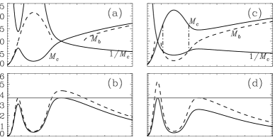
Figure 2: Wind solutions with the streamer geometry for which $f_{\infty}=6$, $f_{M}=14$, $r_{C}=3$$R_{\odot}$, and $\delta=0.7$$R_{\odot}$. In the left and right columns, $T$ is 1.2 and 1.3 MK, respectively. Panels (a) and (c) present the $r-$dependence of the Mach number $M$, while (b) and (d) give that of $D$. The solid (dashed) lines represent the continuous (broken) solutions. In (b) and (d), the horizontal lines give $1/e$ for comparison. Standing shocks are allowed only when the two curves $1/M_{c}$ and $M_{b}$ intersect.

Figure 2 illustrates our solution procedure, giving the radial dependence of the Mach number $M$ ((a) and (c)) and $D$ ((b) and (d)). In Figs.2b and 2d, the light horizontal lines represent $1/e$. The solid and dashed lines correspond to the continuous and broken solutions, respectively. In addition to $M$, Figs.2a and 2c also give $1/M_{c}$. Figures 2a and 2b are for $T=1.2$ MK, while Figs.2c and 2d are for $T=1.3$ MK. In both cases the tube parameters are $f_{\infty}=6$, $f_{M}=14$, $r_{C}=3$$R_{\odot}$, and $\delta=0.7$$R_{\odot}$. Consider now Figs.2a and 2b. It is seen that both curves in Fig.2b exhibit three local extrema, whose locations correspond to the CPs. This follows from that $dD/dy=0$ at any CP (see Eq.(8)). Furthermore, the global maximum of $D$ is attained at the outermost CP, located at 4.89$R_{\odot}$. Therefore when the innermost CP is chosen as the SP, $D>1/e$ around the outermost CP for $4.2\leq r\leq 6.51$$R_{\odot}$. Recalling that $W(-D)$ is real-valued only when $-D\geq-1/e$, one readily understands that in this interval choosing the innermost CP as the SP does not result in a solution to Eq.(1). Figure 2a also shows that the curve $1/M_{c}$ does not intersect $M_{b}$, indicating the solution to Eq.(1) is unique and is the continuous one.

The situation changes when $T=1.3$ MK. Now the global maximum of $D$ is attained at the innermost CP, located at 1.75$R_{\odot}$ (Fig.2d). Choosing the outermost CP as the SP leads to that $D>1/e$ in the interval [1.53, 1.98]$R_{\odot}$ where there is no solution (Fig.2c). However, two standing shocks are now allowed, since two crossings exist between the curves $1/M_{c}$ and $M_{b}$, located at 2.11 and 3.96$R_{\odot}$, respectively. Hence in addition to the continuous one ($M_{c}$ adopting the innermost CP as the SP), two additional solutions exist to Eq.(1): both start with $M_{c}$ but one connects to $M_{b}$ at the inner crossing, the other connects to $M_{b}$ at the outer one.

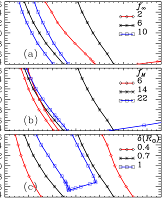
Figure 3: Regions in the $T-r_{C}$ space where standing shocks are allowed, shown as the area bounded by the two curves in same color. The results are obtained by varying $f_{\infty}$, $f_{M}$ and $\delta$ respectively, the rest of the parameters are fixed at their reference values $f_{\infty}=6$, $f_{M}=14$, $\delta=0.7$$R_{\odot}$.

Although Eq.(1) permits solutions with shocks, and time-dependent simulations suggest these steady-state solutions can be attainedHasanVenka_82 ; HabbalRosner_84 ; Habbal_etal_94 ; MarschTu_97 , one may still question whether the shock solutions can stand the sensitivity test similar toLeerHolzer_90 which showed standing shocks in the solar wind from the center of coronal holes are very unlikely, for the parameter range allowing shock solutions is extremely limited. To see whether the same happens with the streamer geometry, we note that given $f_{\infty}$, $f_{M}$ and $\delta$, shock solutions are allowed only in the area bounded by two curves in the $[T,r_{C}]$ space. Figure 3 presents a series of such curves obtained by varying (a) $f_{\infty}$, (b) $f_{M}$, and (c) $\delta$ about the reference values $f_{\infty}=6$, $f_{M}=14$, and $\delta=0.7$$R_{\odot}$. (In what follows, the temperatures are in MK, $r_{C}$ and $\delta$ in $R_{\odot}$.) Let us first examine the cases with reference values (the black curves connecting asterisks). Figure 3 shows that the area bounded by the two curves is rather broad, and with increasing $r_{C}$, both curves are shifted towards lower temperatures, indicating streamers whose cusps are located higher in the corona are more likely associated with standing shocks. For instance, when the cusp is located at $3.6$$R_{\odot}$, the slow wind may possess standing shocks as long as $0.91\leq T\leq 2.04$, which actually tends to be lower than the often-quoted values of coronal temperatures. On the other hand, even for the lowest cusp height examined ($r_{C}=2.4$$R_{\odot}$), the temperature range is $[1.74,2.80]$, still largely compatible with the observational range.

Figure 3a examines the effects of varying $f_{\infty}$. It is seen that while $f_{\infty}$ decreases from its reference value to $2$ (the red curves), the $T$ range allowing shocks increases significantly. Actually for $r_{C}\geq 2.5$, in the examined temperature range there virtually exists no upper bound for shocks to occur. Take $r_{C}=3.6$ for instance. Shock solutions take place as long as $T\geq 1.35$. On the contrary, increasing $f_{\infty}$ to $10$ (the blue curves) makes shocks appear in a much narrower $T$ range (the width is $\sim 0.3$). The effects of varying $f_{M}$ are shown in Fig.3b, which shows that increasing $f_{M}$ considerably broadens the area allowing standing shocks. For example, with $f_{M}$ increasing from $6$ to $14$, the width along the $T$-axis of the area increases from $\sim 0.1$ to $1.1$. When $f_{M}$ further increases to $22$, this width increases dramatically from $\sim 0.88$ at $r_{c}=2.4$ to $\gtrsim 2.9$ for $r_{c}\geq 2.6$. Figure 3c shows what happens when $\delta$ changes, where it is seen that increasing $\delta$ reduces the range of $T$ where shocks are allowed. For instance, with $r_{C}=3.0$, this range for $\delta=0.4$ ($\delta=1$) is $[1.27,3.21]$ ($[1.55,2.26]$), while the range for the reference value $\delta=0.7$ lies in between. It is interesting to note that for $\delta=1$, at $r_{C}\sim 2.68$ the upper bound for $T$ (the right blue curve) changes its slope dramatically, and for $r_{C}\leq 2.53$ no shock solutions exist. For $2.53\leq r_{C}\leq 2.68$, it turns out that on the right of the right blue curve actually no solution exists, since now only two critical points exist and neither of them corresponds to a $D\leq 1/e$ throughout the computational domain (see Eq.(7)). This is different from the portion $r_{C}\geq 2.68$, where on the right of the right blue curve there does exist a solution which is the continuous one. Putting the three panels together, one may see that for most combinations of tube parameters, the area in the $T-r_{C}$ space supporting standing shocks is substantial. Hence with the streamer geometry, standing shocks in the inner slow wind seem physically accessible.

It is not easy to exhaust the possible tube parameters and the consequent changes in shock properties. Let us instead discuss only the shocks found, examining their detectability. First, $\delta\rho$, the density jump relative to the upstream value, is up to $8$, a result of the isothermal assumption exceeding the nominal upper limit of $4$ for adiabatic gases. As shown byEsserHabbal_90 , a $\delta\rho$ of $\sim 2.3$ at a standing shock produces an enhancement in the polarized brightness intensity that is only marginally detectable. A $\delta\rho$ of $8$ certainly makes such detections easier, but one can not say this for sure without constructing detailed observables. Second, by conserving angular momentum a coronal shock also produces a discontinuity in the azimuthal flow speed $v_{\phi}$, leading in principle to measurable Doppler shifts in H I Ly $\alpha$. However, the jump in $v_{\phi}$ turns out $\lesssim 4$ km/s, discerning which is way beyond the sensitivity of SOHO/UVCS, whose spectral resolution of $0.23$ Å translates into $\sim 57$ km/s.

The isothermal assumption needs some justification. First, it is not far from reality. The UVCS measurements of the H I Ly $\alpha$ emission from an equatorial streamerStrachan_etal_02 showed that the proton kinetic temperature $T_{p}$ in the stalk decreases only mildly from 1.45 MK at 3.6$R_{\odot}$ to 1.3 MK at 5.1$R_{\odot}$ (their Fig.3b). If the stalk and one of streamer legs are on the same flow tube, then Fig.4b inStrachan_etal_02 shows that $1.41\leq T_{p}\leq 2.09$ MK at 2.33$R_{\odot}$ (the leftmost two open circles and rightmost two solid ones in their Fig.4d). As for $T_{e}$, the electron-scattered H I Ly$\alpha$ measured by UVCS yielded a $T_{e}$ of $1.1\pm 0.3$ MK at 2.7$R_{\odot}$Fineschi_etal_98 . Although for a streamer, this value may serve to estimate $T_{e}$ in flowing regions at similar heights. Direct $T_{e}$ measurements above that distance are sparse. Nonetheless, multi-fluid MHD models indicate that $T_{e}$ ranges from 0.8 MK at 3$R_{\odot}$ to 0.65 MK at 5$R_{\odot}$ (Fig.3d inLi_etal_06 ). The mean of $T_{e}$ and $T_{p}$, the temperature $T$ in this study is thus $\sim 1.1-1.8$ MK at 2.3$R_{\odot}$ and decreases to $\sim 1$ MK at $5$$R_{\odot}$. Furthermore, $T$ at the slow wind source region is $\sim 0.8-1.2$ MK, be this source in a coronal hole or in its neighboring quiet SunHabbal_etal_93 . Second, introducing a more complete energy equation, as was done inHabbal_etal_94 for a coronal-hole flow, will likely strengthen rather than weaken our conclusion. That study shows that introducing thermal conduction and two-fluid effects allows for a much broader parameter range supporting standing shocks, compared with isothermal and polytropic computations.

References

- (1) Holzer T E 1977 J. Geophys. Res. 82 23
- (2) Hasan S S and Venkatakrishnan P 1982 Sol. Phys. 80 385
- (3) Habbal S R and Tsinganos K 1983 J. Geophys. Res. 88 1965
- (4) Habbal S R and Rosner R 1984 J. Geophys. Res. 89 10645
- (5) Habbal S R, Hu Y Q and Esser R 1994 J. Geophys. Res. 99 8465
- (6) Leer E and Holzer T E 1990 Astrophys. J. 358 680
- (7) Marsch E and Tu C-Y 1997 Sol. Phys. 176 87
- (8) Wang Y-M, Ko Y-K and Grappin R 2009 Astrophys. J. 691 760
- (9) Wang Y-M and Sheeley N R Jr. 1990 Astrophys. J. 355 726
- (10) Cranmer S R 2004 Am. J. Phys. 72 1397
- (11) Corless R M, Gonnet G H, Hare D E G, Jeffrey D J and Knuth D E 1996 Adv. Comput. Math. 5 329
- (12) Velli M 2001 Astrophys. Space Sci. 277 157
- (13) Esser R and Habbal S R 1990 Sol. Phys. 129 153
- (14) Strachan L, Suleiman R, Panasyuk A V, Biesecker D A and Kohl J L 2002 Astrophys. J. 571 1008
- (15) Fineschi S , Gardner L D, Kohl J L, Romoli M and Noci G 1998 Proc. SPIE 3443 67
- (16) Habbal S R, Esser R and Arndt M B 1993 Astrophys. J. 413 435
- (17) Li B, Li X and Labrosse N 2006 J. Geophys. Res. 111 A08106