Perturbation theory for plasmonic eigenvalues

Abstract

We develop a perturbative approach for calculating, within the quasistatic approximation, the shift of surface resonances in response to a deformation of a dielectric volume. Our strategy is based on the conversion of the homogeneous system for the potential which determines the plasmonic eigenvalues into an inhomogeneous system for the potential’s derivative with respect to the deformation strength, and on the exploitation of the corresponding compatibility condition. The resulting general expression for the first-order shift is verified for two explicitly solvable cases, and for a realistic example of a deformed nanosphere. It can be used for scanning the huge parameter space of possible shape fluctuations with only quite small computational effort.

I Introduction

Recent advances in plasmonics, i.e., in the use of surface plasmons for subwavelength optics, BarnesEtAl03 ; MaierAtwater05 ; Ozbay06 have led to renewed interest in the physics of plasmon excitations bound to smooth or rough surfaces. Raether88 In particular, it has been proposed to transport electromagnetic energy along linear chains of nanoparticles, QuintenEtAl98 possibly embedded in a gain medium, Citrin06 and proof-of-principle experiments have been made. BrongersmaEtAl00 ; MaierEtAl01 ; MaierEtAl03 In such setups, fabrication-induced shape imperfections of the nanoparticles inevitably will result in slight shifts of their resonance frequencies, and it might be crucial to estimate the maximum size of such fluctuations which can still be tolerated. deWaeleEtAl07 Although sophisticated numerical methods for computing the optical response of nanoparticles do exist, MartinEtAl95 ; HohenesterKrenn05 it would still be helpful to have a flexible analytical tool which exploits the fact that the shape of an unintentionally deformed nanoparticle is close to some theoretical ideal, as this tool would allow one to explore the huge parameter space of possible perturbations in a computationally cheap manner.

In the present paper we develop such a perturbative approach to the computation of surface resonances. Our strategy is quite general, relying on concepts borrowed from differential geometry. doCarmo76 The mathematical arguments are given in the following Sec. II; some technical details have been deferred to Appendix A. The main results are the expressions (26) and (28), which quantify the shifts of the resonance frequencies to first order in the deformation strength. Section III then provides three illustrative examples. The first two of these make contact with analytically solvable models, thus helping to gain confidence in the formalism, while the third one is a more realistic application to a deformed nanosphere for which no closed analytical solution is available. This necessitates to consider the splitting of degenerate modes, which is done in Appendix B. The paper ends with some concluding remarks in Sec. IV.

II Perturbation theory for plasmonics

Consider a volume $\Omega\subset\mathbb{R}^{3}$ filled with a dielectric medium which is characterized by an isotropic, frequency-dependent dielectric function $\epsilon(\omega)$; this volume $\Omega$ be surrounded by vacuum. We employ the quasistatic approximation, which is valid if the characteristic linear extensions of $\Omega$ are small in comparison with the wavelengths of impinging radiation, and thus captures essential features of nonretarded plasmon dynamics in small nanoparticles. HohenesterKrenn05 ; LiEtAl03 ; ParkStroud04 ; NordlanderEtAl04 ; KlimovGuzatov07 The Fourier components $u({\bf r}|\omega)$ of the potential then are given by the solutions to the set of equations

$$\Delta u = 0\quad\text{in }\mathbb{R}^{3}\setminus\partial\Omega$$ (1)

$$u_{-}-u_{+} = 0\quad\text{on }\partial\Omega$$ (2)

$$\epsilon\partial_{n}u_{-}-\partial_{n}u_{+} = 0\quad\text{on }\partial\Omega\;.$$ (3)

Here $u_{-}$ is the restriction of $u$ to the interior $\Omega$ and $u_{+}$ its restriction to the open exterior $\mathbb{R}^{3}\setminus\overline{\Omega}$; both $u_{-}$ and $u_{+}$ are smooth everywhere except at the boundary $\partial\Omega$. We stipulate that $\partial\Omega$ be sufficiently smooth to substantiate the following operations, and suppress the dependence of $u$ on the frequency $\omega$ altogether. The expressions $\partial_{n}u_{\pm}={\bf n}\cdot{\bf\nabla}u_{\pm}$ in Eq. (3) are the derivatives of the potential in the direction of the outward unit normal ${\bf n}$.

Observe that at this point the knowledge of the dielectric function $\epsilon(\omega)$ is not yet required. Rather, we take $\epsilon$ on the l.h.s. of Eq. (3) as a real number and regard it as an eigenvalue, henceforth dubbed as plasmonic eigenvalue, if the system (1) – (3) with that particular $\epsilon$ possesses a nontrivial solution $u$ which vanishes at least quadratically with increasing distance from $\partial\Omega$. This nomenclature is formally justified by reformulating the system (1) – (3) in terms of Dirichlet-to-Neumann operators, so that the desired values of $\epsilon$ explicitly appear as inverse eigenvalues of a combination of such operators. GrieserRueting09 This somewhat unfamiliar view offers conceptual advantages: On the one hand, the material-specific aspects of the problem, embodied in the function $\epsilon(\omega)$, are separated from the geometric ones; only these geometric aspects matter when studying deformations of $\Omega$. On the other hand, standard theorems concerning the behavior of eigenvalues of linear operators under perturbations can now be employed. After such a plasmonic eigenvalue has been found for a particular geometry, i.e., for some domain $\Omega$ with a given shape, that eigenvalue then determines the frequency $\omega_{\rm s}$ of a surface resonance through the equation $\epsilon={\rm Re}\big{(}\epsilon(\omega_{\rm s})\big{)}$. For example, a half space with planar boundary $\partial\Omega$ yields $\epsilon=-1$, and the dielectric function can be taken as

$$\epsilon(\omega)=1-\frac{\omega_{\rm p}^{2}}{\omega^{2}}$$ (4)

for metallic materials with plasma frequency $\omega_{\rm p}$, describing the free electron motion. This then leads to the familiar expression $\omega_{\rm s}=\omega_{\rm p}/\sqrt{2}$ for the surface plasmon resonance at a planar metal-vacuum interface in the quasistatic limit. Raether88 Typical plasma frequencies for good conductors are on the order of $10^{16}$ s^-1.

We now consider the response of a plasmonic eigenvalue $\epsilon$ to a small deformation of $\Omega$. This deformation is modeled in terms of a shape function $a:\partial\Omega\to\mathbb{R}$ and a dimensionless parameter $h$, such that the surface of the deformed volume is given by

$$\partial\Omega(h)=\{{\bf r}+ha({\bf r})\,{\bf n}({\bf r}):\,{\bf r}\in\partial\Omega\}\;.$$ (5)

We assume that one has solutions $\epsilon(h)$, $u({\bf r},h)$ to the problem (1) – (3) with $\Omega$ replaced by $\Omega(h)$, and that $\epsilon(h)$ and $u({\bf r},h)$ depend differentiably on $h$. We denote the derivatives in $h$ by a dot and write $\dot{\epsilon}=\dot{\epsilon}(0)$ and $\dot{u}({\bf r})=\dot{u}({\bf r},0)$ for brevity.

In what follows we derive a system of equations for $\dot{\epsilon}$ and $\dot{u}({\bf r})$, and therefrom an explicit expression for $\dot{\epsilon}$. To this end, we take the derivative of the system (1) – (3) with respect to $h$. First, for any ${\bf r}\not\in\partial\Omega=\partial\Omega(0)$ one has ${\bf r}\not\in\partial\Omega(h)$ for $h$ sufficiently close to zero; therefore, Eq. (1) readily yields

$$\Delta\dot{u}=0\quad\text{in }\mathbb{R}^{3}\setminus\partial\Omega\;.$$ (6)

Next we differentiate Eq. (2). In a more explicit form, this equation reads

$$u_{-}({\bf r}+ha({\bf r})\,{\bf n}({\bf r}),h)-u_{+}({\bf r}+ha({\bf r})\,{\bf n}({\bf r}),h)=0$$ (7)

and hence gives

$$a{\bf n}\cdot{\bf\nabla}u_{-}+\dot{u}_{-}-\left(a{\bf n}\cdot{\bf\nabla}u_{+}+\dot{u}_{+}\right)=0$$ (8)

or

$$\dot{u}_{-}-\dot{u}_{+} = a{\bf n}\cdot{\bf\nabla}u_{+}-a{\bf n}\cdot{\bf\nabla}u_{-}$$ (9)

$$= (\epsilon-1)a\partial_{n}u_{-}\;,$$

where Eq. (3) has been used for eliminating $u_{+}$.

Similarly we differentiate Eq. (3), keeping in mind that $\partial_{n}u_{\pm}={\bf n}\cdot{\bf\nabla}u_{\pm}$, and taking into account that ${\bf n}$ also depends on $h$. Thus, one has

$$({\bf n}\cdot{\bf\nabla}u_{\pm})\dot{}={\bf\dot{n}}\cdot{\bf\nabla}u_{\pm}+{\bf n}\cdot({\bf\nabla}u_{\pm})\dot{}\;.$$ (10)

The required derivatives ${\bf\dot{n}}$ and ${\bf n}\cdot({\bf\nabla}u_{\pm})\dot{}$ are calculated in Appendix A. According to Eq. (67), ${\bf\dot{n}}=-{\bf\nabla}_{\partial}a$ coincides with the negative gradient of the shape function inside the surface $\partial\Omega$, while Eq. (76) expresses ${\bf n}\cdot({\bf\nabla}u_{\pm})\dot{}$ in terms of the Laplace-Beltrami operator $\Delta_{\partial}=\operatorname{div}_{\partial}{\bf\nabla}_{\partial}$ applied to $u_{\pm}$, and the mean curvature $H$ of $\partial\Omega$. Combining these results, we find

$$({\bf n}\cdot{\bf\nabla}u_{\pm})\dot{}$$ (11)

$$= -{\bf\nabla}_{\partial}a\cdot{\bf\nabla}_{\partial}u_{\pm}-a\Delta_{\partial}u_{\pm}+2aH\partial_{n}u_{\pm}+\partial_{n}\dot{u}_{\pm}$$

$$= -\operatorname{div}_{\partial}(a{\bf\nabla}_{\partial}u_{\pm})+2aH\partial_{n}u_{\pm}+\partial_{n}\dot{u}_{\pm}\;.$$

Thus, taking the $h$-derivative of Eq. (3) leads to

$$(\epsilon\partial_{n}u_{-}-\partial_{n}u_{+})\dot{} = \dot{\epsilon}\partial_{n}u_{-}+\epsilon(\partial_{n}u_{-})\dot{}-(\partial_{n}u_{+})\dot{}$$ (12)

$$= \dot{\epsilon}\partial_{n}u_{-}$$

$$-\operatorname{div}_{\partial}\left(a(\epsilon{\bf\nabla}_{\partial}u_{-}-{\bf\nabla}_{\partial}u_{+})\right)$$

$$+2aH(\epsilon\partial_{n}u_{-}-\partial_{n}u_{+})$$

$$+\epsilon\partial_{n}\dot{u}_{-}-\partial_{n}\dot{u}_{+}\;.$$

The l.h.s. now vanishes identically, and the third term on the r.h.s. vanishes because of Eq. (3) itself. Moreover, since $u_{+}=u_{-}$ on $\partial\Omega$ according to Eq. (2), and ${\bf\nabla}_{\partial}$ differentiates inside $\partial\Omega$ only, we can replace ${\bf\nabla}_{\partial}u_{+}$ by ${\bf\nabla}_{\partial}u_{-}$ in the second term, finally leaving us with

$$\epsilon\partial_{n}\dot{u}_{-}-\partial_{n}\dot{u}_{+}=-\dot{\epsilon}\partial_{n}u_{-}+(\epsilon-1)\operatorname{div}_{\partial}(a{\bf\nabla}_{\partial}u_{-})\;.$$ (13)

In summary, the differentiation of the homogeneous system (1) – (3) has led to the inhomogeneous system

$$\Delta\dot{u} = 0\quad\text{in }\mathbb{R}^{3}\setminus\partial\Omega$$ (14)

$$\dot{u}_{-}-\dot{u}_{+} = F\quad\text{on }\partial\Omega$$ (15)

$$\epsilon\partial_{n}\dot{u}_{-}-\partial_{n}\dot{u}_{+} = -\dot{\epsilon}\partial_{n}u_{-}+G\quad\text{on }\partial\Omega\;,$$ (16)

where

$$F = (\epsilon-1)a\partial_{n}u_{-}$$ (17)

$$G = (\epsilon-1)\operatorname{div}_{\partial}(a{\bf\nabla}_{\partial}u_{-})\;.$$ (18)

Since the homogeneous system has a nontrivial solution (the given $u$), its inhomogeneous descendant can admit a solution only if the right hand sides $F$, $-\dot{\epsilon}\partial_{n}u_{-}+G$ satisfy a certain compatibility condition. Since by assumption there is a solution (the $h$-derivative of the given family $u({\bf r},h)$), this condition actually is fulfilled, and yields an expression for $\dot{\epsilon}$. For deriving this expression, we start from $\Delta u_{-}=\Delta\dot{u}_{-}=0$ in $\Omega$. Green’s formula then gives

$$0 = \int_{\Omega}\!{\rm d}^{3}r\,\big{(}u_{-}\Delta\dot{u}_{-}-(\Delta u_{-})\dot{u}_{-}\big{)}$$ (19)

$$= \int_{\partial\Omega}\!{\rm d}^{2}S\,\big{(}u_{-}\partial_{n}\dot{u}_{-}-(\partial_{n}u_{-})\dot{u}_{-}\big{)}\;,$$

where ${\rm d}^{2}S$ denotes the surface area element. Thus, one has

$$\int_{\partial\Omega}\!{\rm d}^{2}S\,u_{-}\partial_{n}\dot{u}_{-}=\int_{\partial\Omega}\!{\rm d}^{2}S\,(\partial_{n}u_{-})\dot{u}_{-}\;;$$ (20)

a corresponding identity holds for $u_{+}$, $\dot{u}_{+}$. Therefore,

$$\int_{\partial\Omega}\!{\rm d}^{2}S\,\big{(}u_{-}\epsilon\partial_{n}\dot{u}_{-}-u_{+}\partial_{n}\dot{u}_{+}\big{)}$$ (21)

$$= \int_{\partial\Omega}\!{\rm d}^{2}S\,\big{(}\epsilon(\partial_{n}u_{-})\dot{u}_{-}-(\partial_{n}u_{+})\dot{u}_{+}\big{)}\;.$$

Since $u_{-}=u_{+}$ on $\partial\Omega$, the l.h.s. becomes

$$\int_{\partial\Omega}\!{\rm d}^{2}S\;u_{-}\big{(}\epsilon\partial_{n}\dot{u}_{-}-\partial_{n}\dot{u}_{+}\big{)}=\int_{\partial\Omega}\!{\rm d}^{2}S\;u_{-}\big{(}-\dot{\epsilon}\partial_{n}u_{-}+G\big{)}\;.$$ (22)

On the other hand, since $\partial_{n}u_{+}=\epsilon\partial_{n}u_{-}$ on $\partial\Omega$, the r.h.s. of Eq. (21) takes the form

$$\int_{\partial\Omega}\!{\rm d}^{2}S\;\epsilon(\partial_{n}u_{-})\left(\dot{u}_{-}-\dot{u}_{+}\right)=\epsilon\int_{\partial\Omega}\!{\rm d}^{2}S\;(\partial_{n}u_{-})F\;.$$ (23)

Equating these two expressions (22) and (23), and solving for $\dot{\epsilon}$, we obtain

$$\dot{\epsilon}=\frac{\int_{\partial\Omega}\!{\rm d}^{2}S\;u_{-}G-\epsilon\int_{\partial\Omega}\!{\rm d}^{2}S\,(\partial_{n}u_{-})F}{\int_{\partial\Omega}\!{\rm d}^{2}S\;u_{-}\partial_{n}u_{-}}\;.$$ (24)

Inserting the formulas (17) and (18) for $F$ and $G$, and performing an integration by parts, the numerator reduces to

$$\int_{\partial\Omega}\!{\rm d}^{2}S\;u_{-}(\epsilon-1)\operatorname{div}_{\partial}(a{\bf\nabla}_{\partial}u_{-})$$ (25)

$$-\epsilon\int_{\partial\Omega}\!{\rm d}^{2}S\;(\partial_{n}u_{-})(\epsilon-1)a\partial_{n}u_{-}$$

$$= (1-\epsilon)\int_{\partial\Omega}\!{\rm d}^{2}S\,a\big{(}({\bf\nabla}_{\partial}u_{-})^{2}+\epsilon(\partial_{n}u_{-})^{2}\big{)}\;.$$

Thus, the desired expression for the first-order change of the plasmonic eigenvalue $\epsilon$ with the deformation strength $h$ finally reads

$$\dot{\epsilon}=(1-\epsilon)\frac{\int_{\partial\Omega}\!{\rm d}^{2}S\;a\left(({\bf\nabla}_{\partial}u_{-})^{2}+\epsilon(\partial_{n}u_{-})^{2}\right)}{\int_{\partial\Omega}\!{\rm d}^{2}S\,u_{-}\partial_{n}u_{-}}\;.$$ (26)

This is the principal result of the present work. Observe that $\Delta u_{-}=0$ implies

$$\int_{\partial\Omega}\!{\rm d}^{2}S\,u_{-}\partial_{n}u_{-}=\int_{\Omega}\!{\rm d}^{3}r\,(\nabla u_{-})^{2}\;,$$ (27)

so that the denominator is positive. Of course, $\dot{\epsilon}$ can likewise be expressed entirely in terms of $u_{+}$:

$$\dot{\epsilon}=(1-\epsilon)\frac{\int_{\partial\Omega}\!{\rm d}^{2}S\;a\left(\epsilon({\bf\nabla}_{\partial}u_{+})^{2}+(\partial_{n}u_{+})^{2}\right)}{\int_{\partial\Omega}\!{\rm d}^{2}S\,u_{+}\partial_{n}u_{+}}\;.$$ (28)

III Applications

Consider an infinite half-space geometry with the dielectric medium filling the volume $z<0$, so that its boundary is given by the plane $z=0$. Let $\bm{\kappa}=(k_{x},k_{y})$ be a two-dimensional wave vector, with $\kappa=\sqrt{k_{x}^{2}+k_{y}^{2}}$. Solutions to Laplace’s equation (1) which vanish for $z\to\pm\infty$ then are given by

$$u_{+}({\bf r}) = \int\!\frac{{\rm d}^{2}\kappa}{(2\pi)^{2}}\,A(\bm{\kappa})\,{\rm e}^{{\rm i}\bm{\kappa}\cdot\mathbf{x}-\kappa z}$$ (29)

$$u_{-}({\bf r}) = \int\!\frac{{\rm d}^{2}\kappa}{(2\pi)^{2}}\,B(\bm{\kappa})\,{\rm e}^{{\rm i}\bm{\kappa}\cdot\mathbf{x}+\kappa z}\;,$$ (30)

with $\mathbf{x}=(x,y)$ and ${\bf r}=(x,y,z)$, and the continuity condition (2) yields $B(\bm{\kappa})=A(\bm{\kappa})$. Moreover, since $u_{\pm}$ is real, one has $A^{*}(\bm{\kappa})=A(-\bm{\kappa})$. At this point, the amplitudes $A(\bm{\kappa})$ describing the excitations at an exactly planar surface are arbitrary. The normal and the in-plane derivatives at $z=0$ then are

$$\partial_{n}u_{\pm} = \mp\int\!\frac{{\rm d}^{2}\kappa}{(2\pi)^{2}}\,A(\bm{\kappa})\,\kappa\,{\rm e}^{{\rm i}\bm{\kappa}\cdot\mathbf{x}}$$ (31)

$${\bf\nabla}_{\partial}u_{\pm} = \int\!\frac{{\rm d}^{2}\kappa}{(2\pi)^{2}}\,A(\bm{\kappa})\,({\rm i}\bm{\kappa})\,{\rm e}^{{\rm i}\bm{\kappa}\cdot\mathbf{x}}\;,$$ (32)

respectively, so that the condition (3) immediately provides the well known eigenvalue $\epsilon=-1$ for this particular geometry. We write

$$(\partial_{n}u_{\pm})^{2} = \int\!\frac{{\rm d}^{2}\kappa}{(2\pi)^{2}}\int\!\frac{{\rm d}^{2}\kappa^{\prime}}{(2\pi)^{2}}A(\bm{\kappa})A^{*}(\bm{\kappa}^{\prime})\,(\kappa\kappa^{\prime})\,{\rm e}^{{\rm i}(\bm{\kappa}-\bm{\kappa}^{\prime})\cdot\mathbf{x}}$$

$$({\bf\nabla}_{\partial}u_{\pm})^{2} = \int\!\frac{{\rm d}^{2}\kappa}{(2\pi)^{2}}\int\!\frac{{\rm d}^{2}\kappa^{\prime}}{(2\pi)^{2}}A(\bm{\kappa})A^{*}(\bm{\kappa}^{\prime})\,(\bm{\kappa}\cdot\bm{\kappa}^{\prime})\,{\rm e}^{{\rm i}(\bm{\kappa}-\bm{\kappa}^{\prime})\cdot\mathbf{x}}$$

together with

$$u_{\pm}\partial_{n}u_{\pm}=\mp\int\!\frac{{\rm d}^{2}\kappa}{(2\pi)^{2}}\int\!\frac{{\rm d}^{2}\kappa^{\prime}}{(2\pi)^{2}}A(\bm{\kappa})A^{*}(\bm{\kappa}^{\prime})\,\kappa^{\prime}\,{\rm e}^{{\rm i}(\bm{\kappa}-\bm{\kappa}^{\prime})\cdot\mathbf{x}}\;,$$

giving

$$\int_{\partial\Omega}\!{\rm d}^{2}S\,u_{\pm}\partial_{n}u_{\pm}=\mp\int\!\frac{{\rm d}^{2}\kappa}{(2\pi)^{2}}\,|A(\bm{\kappa})|^{2}\kappa\;.$$ (33)

Now we introduce a small deformation of the planar surface, described by some suitable shape function $a(\mathbf{x})$. The required amplitudes $A(\bm{\kappa})$ consequently are determined by that deformation; the assumption that the exact potential $u_{\pm}({\bf r})$ can still be written in the form (29) or (30) constitutes the Rayleigh hypothesis. FariasMaradudin83 Upon inserting the Fourier transform of the shape function, i.e.,

$$a(\mathbf{x})=\int\!\frac{{\rm d}^{2}\kappa}{(2\pi)^{2}}\,\widehat{a}(\bm{\kappa})\,{\rm e}^{{\rm i}\bm{\kappa}\cdot\mathbf{x}}\;,$$ (34)

und using $\epsilon=-1$ for the unperturbed eigenvalue, either Eq. (26) or its variant (28) readily yields

$$\dot{\epsilon}=2\,\frac{\int\!\frac{{\rm d}^{2}\kappa}{(2\pi)^{2}}\int\!\frac{{\rm d}^{2}\kappa^{\prime}}{(2\pi)^{2}}\,\widehat{a}(\bm{\kappa}^{\prime}-\bm{\kappa})A(\bm{\kappa})A^{*}(\bm{\kappa}^{\prime})\kappa\kappa^{\prime}(\hat{\bm{\kappa}}\cdot\hat{\bm{\kappa}}^{\prime}-1)}{\int\!\frac{{\rm d}^{2}\kappa}{(2\pi)^{2}}\,|A(\bm{\kappa})|^{2}\kappa}\;,$$ (35)

where $\hat{\bm{\kappa}}$ denotes the unit vector in the direction of $\bm{\kappa}$. In particular, if $a(\mathbf{x})=c$, one has $\widehat{a}(\bm{\kappa})=(2\pi)^{2}c\delta(\bm{\kappa})$, so that $\dot{\epsilon}=0$: The plasmonic eigenvalue does not change when the entire surface plane is displaced by some amount $c$.

On the other hand, there exists an exact integral equation for determining the amplitudes $A(\bm{\kappa})$ associated with a given surface deformation, derived by Farias and Maradudin on the basis of the Rayleigh hypothesis: FariasMaradudin83

$$\frac{\epsilon+1}{\epsilon-1}A(\bm{\kappa}^{\prime})=\int\!\frac{{\rm d}^{2}\kappa}{(2\pi)^{2}}\,J(\kappa^{\prime}-\kappa|\bm{\kappa}^{\prime}-\bm{\kappa})(1-\hat{\bm{\kappa}}\cdot\hat{\bm{\kappa}}^{\prime})\kappa A(\bm{\kappa})$$ (36)

with

$$J(\alpha|\mathbf{q})=\frac{1}{\alpha}\int\!{\rm d}^{2}S\,{\rm e}^{-{\rm i}\mathbf{q}\cdot\mathbf{x}}\big{(}\exp(\alpha\,ha(\mathbf{x}))-1\big{)}\;;$$ (37)

this has been applied by Maradudin and Visscher to the study of particular perturbations of planar surfaces. MaradudinVisscher85 Expanding the latter expression (37) to first order in $h$ gives

$$J(\alpha|\mathbf{q})=h\widehat{a}(\mathbf{q})+\mathcal{O}(h^{2})\;,$$ (38)

so that Eq. (36) becomes

$$\frac{\epsilon+1}{\epsilon-1}A(\bm{\kappa}^{\prime})=h\int\!\frac{{\rm d}^{2}\kappa}{(2\pi)^{2}}\,\widehat{a}(\bm{\kappa}^{\prime}-\bm{\kappa})(1-\hat{\bm{\kappa}}\cdot\hat{\bm{\kappa}}^{\prime})\kappa A(\bm{\kappa})$$ (39)

for sufficiently weak perturbations. Recalling that the unperturbed eigenvalue is $-1$, we insert $\epsilon=-1+\mathcal{O}(h)$ into the denominator on the l.h.s. Multiplying both sides by $A^{*}(\bm{\kappa}^{\prime})\kappa^{\prime}$, integrating, and rearranging then yields

$$\epsilon=-1+h\dot{\epsilon}+\mathcal{O}(h^{2})\;,$$ (40)

with $\dot{\epsilon}$ indeed formally equal to the previous Eq. (35). Thus, our perturbative result is consistent with the formula (36).

A second example which allows one to confirm the validity of the perturbative approach by analytical means is provided by the deformation of a dielectric sphere of radius $R$ into a spheroid. In this case the unperturbed potential is written as

$$u_{+}({\bf r}) = \sum_{\ell=1}^{\infty}A_{\ell}r^{-(\ell+1)}Y_{0}^{\ell}(\vartheta)$$

$$u_{-}({\bf r}) = \sum_{\ell=0}^{\infty}B_{\ell}r^{\ell}Y_{0}^{\ell}(\vartheta)\;,$$ (41)

valid for $r\geq R$ and $r\leq R$, respectively. Here $Y_{m}^{\ell}$ denote the familiar spherical harmonics. The restriction to these basis functions with $m=0$, which do not depend on the azimuthal angle $\varphi$, confines us to deformations which preserve the rotation symmetry around the $z$-axis. From condition (2) one gets $B_{\ell}=A_{\ell}R^{-(2\ell+1)}$, and Eq. (3) then leads to the eigenvalues

$$\epsilon_{\ell}=-\frac{\ell+1}{\ell}\;.$$ (42)

In particular, $\epsilon_{1}=-2$ characterizes the dipole resonance. BohrenHuffman98

We deform the sphere into a spheroid oriented along the $z$-axis, employing the shape function

$$a(\vartheta,\varphi)=R\cos^{2}(\vartheta)\;.$$ (43)

Here the choice of the sphere’s radius $R$ as the scale of the deformation is a matter of convenience. The three degenerate dipole modes of the sphere are shifted when the deformation strength $h$ adopts nonzero values, such that the mode associated with the $z$-axis splits off from the two others. For estimating the corresponding change of $\epsilon_{1}$ for small $h$, we use

$$u_{1-}({\bf r})=rY_{0}^{1}(\vartheta)=r\sqrt{\frac{3}{4\pi}}\cos\vartheta\;,$$ (44)

and calculate

$$(\partial_{n}u_{1-})^{2} = \frac{3}{4\pi}\cos^{2}\vartheta$$

$$({\bf\nabla}_{\partial}u_{1-})^{2} = \frac{3}{4\pi}\sin^{2}\vartheta$$

$$u_{1-}\partial_{n}u_{1-} = \frac{3}{4\pi}R\cos^{2}\vartheta$$

on $\partial\Omega$, giving

$$\int_{\partial\Omega}\!{\rm d}^{2}S\,a(\partial_{n}u_{1-})^{2} = \frac{3}{5}R^{3}$$

$$\int_{\partial\Omega}\!{\rm d}^{2}S\,a({\bf\nabla}_{\partial}u_{1-})^{2} = \frac{2}{5}R^{3}$$

$$\int_{\partial\Omega}\!{\rm d}^{2}S\,u_{1-}\partial_{n}u_{1-} = R^{3}\;.$$ (45)

Plugged into Eq. (26), this yields

$$\dot{\epsilon}_{1}=-\frac{12}{5}\;.$$ (46)

This easily obtainable result can be checked against the exactly known expression for the dipolar $z$-mode of a spheroid: BohrenHuffman98

$$\epsilon_{1}=1-\frac{1}{L}\;,$$ (47)

where $L$ denotes the so-called depolarization coefficient, given by LandauLifshitzVIII

$$L(e)=\begin{cases}\frac{1-e^{2}}{e^{3}}\big{(}{\rm artanh}(e)-e\big{)}\;,&h>0\\ \frac{1+e^{2}}{e^{3}}\big{(}e-\arctan(e)\big{)}\;,&h<0\end{cases}$$ (48)

with

$$e^{2}=\begin{cases}1-\frac{1}{(1+h)^{2}}=2h+\mathcal{O}(h^{2})\;,&h>0\\ \frac{1}{(1+h)^{2}}-1=-2h+\mathcal{O}(h^{2})\;,&h<0\;.\end{cases}$$ (49)

Thus, $e^{2}$ becomes small with $h$, allowing us to expand $L(e)$ as

$$L(e)=\begin{cases}\frac{1}{3}-\frac{2}{15}e^{2}+\mathcal{O}(e^{4})\;,&h>0\\ \frac{1}{3}+\frac{2}{15}e^{2}+\mathcal{O}(e^{4})\;,&h<0\;.\end{cases}$$ (50)

Exploiting Eq. (49) one expresses $L$ in terms of $h$, finding

$$L(h)=\frac{1}{3}-\frac{4}{15}h+\mathcal{O}(h^{2})\;.$$ (51)

This tells us that $\epsilon_{1}$, as given by Eq. (47), should be expanded in powers of $(L-1/3)$:

$$\epsilon_{1}=-2+9\left(L-\frac{1}{3}\right)+\mathcal{O}\left(\left(L-\frac{1}{3}\right)^{2}\right)\;.$$ (52)

Inserting Eq. (51), we obtain

$$\epsilon_{1}=-2-\frac{12}{5}h+\mathcal{O}(h^{2})\;,$$ (53)

in accordance with the result (46) of perturbation theory.

The following third example concerns a deformed nanosphere which does not admit an analytical solution in closed form, so that the accuracy achieved by first-order perturbation theory has to be ascertained by comparison with numerical calculations. This is exactly the type of application we have in mind, since here Eqs. (26) and (28) provide a quick and reliable estimate of the possibly detrimental consequences of geometrical imperfections, deWaeleEtAl07 without hard requirements on computational resources. We assume that the ideal sphere is distorted by two Gaussian protrusions, and parametrize its surface as

$$a(\vartheta,\varphi)=R\sum_{i=1,2}f_{i}\exp\left(-\frac{{\rm dist}(\vartheta_{i},\varphi_{i};\vartheta,\varphi)^{2}}{2w_{i}^{2}}\right)\;,$$ (54)

with ${\rm dist}(\vartheta_{i},\varphi_{i};\vartheta,\varphi)$ denoting the dimensionless Euclidean distance between the two points on the unit sphere specified by the angles $\vartheta_{i},\varphi_{i}$ and $\vartheta,\varphi$, respectively. The protrusions’ parameters are chosen, somewhat arbitrarily, as $f_{1}=1.0$, $f_{2}=0.8$ for their amplitudes, $w_{1}=0.7$, $w_{2}=0.65$ for their Gaussian widths, and $\vartheta_{1}=1.1$, $\vartheta_{2}=2.2$ and $\varphi_{1}=4.9$, $\varphi_{2}=0.1$ for their locations. Figure 1 depicts the resulting deformed sphere for the value $h=0.2$ of the overall perturbation strength.

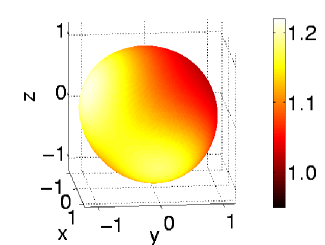
Figure 1: (Color online) Sketch of the particular perturbed nanosphere (54) employed as example for demonstrating the accuracy of the perturbative approach. The deviation of the scaled surface radii $r(\vartheta,\varphi)/R$ from their ideal value $1$ is visualized here for $h=0.2$.

This example also illustrates a further important issue. While the dipole modes of a perfect sphere are threefold degenerate, this degeneracy is removed entirely by the distortion (54). Thus, there now are three branches of dipole-like eigenvalues, and our previous analysis applies to each branch separately, provided the starting point is chosen appropriately: The expressions (26) and (28) refer to the individual branches, if the proper linear combinations of the unperturbed degenerate modes are inserted. The problem how to find these linear combinations is solved in Appendix B. Basically, the numerator of the formula (26) defines a quadratic form of the eigenmodes (see Eq. (87)); the required proper linear combinations of the unperturbed modes are those which diagonalize this form. Their determination, and the evaluation of the ensuing surface integrals determining $\dot{\epsilon}$ for all three branches, does not demand much numerical effort. Figure 2 shows the perturbative results for deformation strengths $-0.25<h<+0.25$ in comparison with data obtained by nonperturbative numerical computations. RuetingUecker09 Quite remarkably, first-order perturbation theory still produces excellent results when the shape variation already is quite substantial, that is, for values of $h$ up to $0.1$; even for $h$ as large as $0.2$ one obtains good estimates.

Figure 2: Numerically computed plasmonic eigenvalues for the dipole modes of the deformed nanosphere depicted in Fig. 1 (crosses), in comparison with the results of first-order perturbation theory (full lines).

IV Concluding remarks

The first-order perturbative expression (26) or (28) for the shift of a plasmonic eigenvalue clearly has a limited range of applicability, insofar as it is restricted to sufficiently weak deformations, but it stands out because of its generality, and easy use. Together with similar results for higher derivatives, Grieser09 one obtains a formal perturbation series

$$\epsilon(h)\sim\epsilon+h\dot{\epsilon}+\frac{1}{2}h^{2}\ddot{\epsilon}+\ldots\;.$$ (55)

Above we have simply assumed the existence of $\epsilon(h)$ and $u({\bf r},h)$. Given a solution at $h=0$, this existence actually follows from the reformulation of the problem in terms of Dirichlet-to-Neumann operators, GrieserRueting09 and from standard perturbation theory for eigenvalues. If $\epsilon$ is $p$-fold degenerate (as in the case of the sphere), then one has $p$ branches $\epsilon^{(i)}$, $u^{(i)}$; $i=1,\ldots,p$. The analysis of Sec. II then applies to each branch separately, with $\dot{\epsilon}^{(i)}$ being given by Eq. (26) or (28) with $u=u^{(i)}$. Here $u^{(1)},\ldots,u^{(p)}$ form a basis of the subspace of degenerate solutions at $h=0$, determined such that they diagonalize the quadratic form given by Eq. (87).

The three examples we have given in Sec. III vary in character, the first two recovering known analytical results and thus confirming the correctness of our formal line of reasoning. The third example, summarized by Figs. 1 and 2, demonstrates the utility of our approach for practical purposes. Here we have dealt with an asymmetrically deformed nanosphere, and obtained fairly good estimates for the shifted dipole modes. If we assume that tolerances on the order of 5% can be met in nanosphere fabrication, first-order perturbation theory thus allows one to quantify the effects of a large variety of possible shape fluctuations with both sufficent accuracy and only small numerical effort.

Appendix A Auxiliary calculations

In this appendix we compute the derivatives entering into the evaluation of Eq. (10) en route to the important result (13). This calculation invokes some notions from differential geometry. doCarmo76 We fix a point ${\bf r}_{0}\in\partial\Omega=\partial\Omega(0)$ and parametrize $\partial\Omega$ near ${\bf r}_{0}$ as ${\bf r}={\bf r}(v,w)$, with ${\bf r}_{0}={\bf r}(0,0)$. It is assumed that the parametrization is such that the tangent vectors ${\bf r}_{v}=\partial_{v}{\bf r}$ and ${\bf r}_{w}=\partial_{w}{\bf r}$ are orthogonal, and have unit length at ${\bf r}_{0}$, and such that the $v$-line (i.e., $v\mapsto{\bf r}(v,0)$) and the $w$-line through ${\bf r}_{0}$ have normal vectors parallel to ${\bf n}$ at ${\bf r}_{0}$ (i.e., have vanishing geodesic curvature).

The curvatures of the $v$-line and the $w$-line are $\kappa_{v}={\bf r}_{vv}\cdot{\bf n}$ and $\kappa_{w}={\bf r}_{ww}\cdot{\bf n}$, respectively. Considering ${\bf n}$ as a function of $v$, $w$, one has

$${\bf r}_{v}\cdot{\bf n}=0$$ (56)

and hence

$${\bf r}_{vv}\cdot{\bf n}+{\bf r}_{v}\cdot{\bf n}_{v}=0\;,$$ (57)

giving

$$\kappa_{v}=-{\bf r}_{v}\cdot{\bf n}_{v}\;;$$ (58)

analogously, $\kappa_{w}=-{\bf r}_{w}\cdot{\bf n}_{w}$.

Note that orthonormality of ${\bf r}_{v}$ and ${\bf r}_{w}$ holds only at ${\bf r}_{0}$, not at nearby points. In the following calculations we always evaluate at $h=0$ after differentiating in $h$, and at ${\bf r}$ = ${\bf r}_{0}$ after differentiating in $v$, $w$.

We now derive an expression for ${\bf\dot{n}}$. The surface $\partial\Omega(h)$ is parametrized by

$${\bf r}(v,w,h)={\bf r}(v,w)+ha(v,w){\bf n}(v,w)\;,$$ (59)

where we abuse notation by considering $a$ and ${\bf n}$ as functions of $v$, $w$. Its unit normal is ${\bf n}={\bf N}/\|{\bf N}\|$, where ${\bf N}={\bf r}_{v}\times{\bf r}_{w}$. At ${\bf r}_{0}$ one has ${\bf n}={\bf N}$ by assumption. Differentiating, one gets

$$\dot{{\bf n}} = \frac{\dot{{\bf N}}}{\|{\bf N}\|}-\frac{{\bf N}}{\|{\bf N}\|^{2}}\left(\frac{{\bf N}}{\|{\bf N}\|}\cdot\dot{{\bf N}}\right)$$ (60)

$$= \frac{1}{\|{\bf N}\|}\left(\dot{{\bf N}}-{\bf n}({\bf n}\cdot\dot{{\bf N}})\right)\;,$$

which states that $\dot{{\bf n}}$ is determined by the tangential part of $\dot{{\bf N}}$. Moreover,

$$\dot{{\bf N}}=\dot{{\bf r}}_{v}\times{\bf r}_{w}+{\bf r}_{v}\times\dot{{\bf r}}_{w}\;.$$ (61)

Since $\dot{{\bf r}}=a{\bf n}$, one has

$$\dot{{\bf r}}_{v}=a_{v}{\bf n}+a{\bf n}_{v}\;.$$ (62)

At ${\bf r}_{0}$, the identity ${\bf n}={\bf r}_{v}\times{\bf r}_{w}$ implies ${\bf n}\times{\bf r}_{w}=-{\bf r}_{v}$ and ${\bf r}_{v}\times{\bf n}=-{\bf r}_{w}$. In addition, ${\bf n}_{v}\times{\bf r}_{w}=({\bf n}_{v}\cdot{\bf r}_{v}){\bf r}_{v}\times{\bf r}_{w}$, because the component of ${\bf n}_{v}$ parallel to ${\bf r}_{w}$ drops out of the vectorial product. (Observe that ${\bf n}\cdot{\bf n}=1$ implies ${\bf n}_{v}\cdot{\bf n}=0$, so that ${\bf n}_{v}$ lies in the span of ${\bf r}_{v}$ and ${\bf r}_{w}$.) Putting this together and using Eq. (58), one finds

$$\dot{{\bf r}}_{v}\times{\bf r}_{w} = \left(a_{v}{\bf n}+a{\bf n}_{v}\right)\times{\bf r}_{w}$$ (63)

$$= -a_{v}{\bf r}_{v}+a({\bf n}_{v}\cdot{\bf r}_{v}){\bf n}$$

$$= -a_{v}{\bf r}_{v}-a\kappa_{v}{\bf n}\;;$$

analogously,

$${\bf r}_{v}\times\dot{{\bf r}}_{w}=-a_{w}{\bf r}_{w}-a\kappa_{w}{\bf n}\;.$$ (64)

Inserting Eqs. (63) and (64) into Eq. (61), we arrive at

$$\dot{{\bf N}}=-\left(a_{v}{\bf r}_{v}+a_{w}{\bf r}_{w}\right)-a\left(\kappa_{v}+\kappa_{w}\right){\bf n}\;.$$ (65)

Now we observe that

$$a_{v}{\bf r}_{v}+a_{w}{\bf r}_{w}={\bf\nabla}_{\partial}a$$ (66)

is the gradient of $a$ as a function in the surface $\partial\Omega$. Since according to Eq. (60) the desired derivative $\dot{{\bf n}}$ is the tangential component of $\dot{{\bf N}}$, we have the compact result

$$\dot{{\bf n}}=-{\bf\nabla}_{\partial}a\;.$$ (67)

Next we calculate ${\bf n}\cdot({\bf\nabla}u)\dot{}$ for $u=u_{+}$ or $u=u_{-}$ at ${\bf r}_{0}$. Starting from

$$({\bf\nabla}u)\dot{}\,({\bf r}) = \left.\frac{\partial}{\partial h}\right|_{h=0}({\bf\nabla}u)({\bf r}+ha({\bf r}){\bf n}({\bf r}),h)$$ (68)

$$= a({\bf n}\cdot{\bf\nabla}){\bf\nabla}u({\bf r})+{\bf\nabla}\dot{u}({\bf r})$$

one finds

$${\bf n}\cdot({\bf\nabla}u)\dot{}=a({\bf n}\cdot{\bf\nabla})^{2}u+\partial_{n}\dot{u}\;.$$ (69)

To simplify notation we assume that coordinates in $\mathbb{R}^{3}$ are chosen such that ${\bf n}=(0,0,1)$ at ${\bf r}_{0}$, reducing the first term on the r.h.s. to $a\partial_{x_{3}}^{2}u$ at ${\bf r}_{0}$. Because $\Delta u=0$, we then have, at ${\bf r}_{0}$,

$${\bf n}\cdot({\bf\nabla}u)\dot{}=-a\left(\partial_{x_{1}}^{2}+\partial_{x_{2}}^{2}\right)u+\partial_{n}\dot{u}\;.$$ (70)

This has to be expressed in terms of derivatives of $u$ inside the surface. We choose the surface coordinates as $v=x_{1}$, $w=x_{2}$, but still write ${\bf r}={\bf r}(v,w)$. Differentiating $u$ twice with respect to $v$,

$$\partial_{v}u({\bf r}(v,w)) = ({\bf r}_{v}\cdot{\bf\nabla})u({\bf r}(v,w))$$

$$\partial_{v}^{2}u({\bf r}(v,w)) = ({\bf r}_{v}\cdot{\bf\nabla})^{2}u({\bf r}(v,w))$$ (71)

$$+({\bf r}_{vv}\cdot{\bf\nabla})u({\bf r}(v,w))\;,$$

and observing ${\bf r}_{v}\cdot{\bf\nabla}=\partial_{x_{1}}$ and ${\bf r}_{vv}=\kappa_{v}{\bf n}$, we get

$$\partial_{v}^{2}u=\partial_{x_{1}}^{2}u+\kappa_{v}\partial_{n}u\;.$$ (72)

Combining this with the analogous equation for $x_{2}$ gives

$$\left(\partial_{x_{1}}^{2}+\partial_{x_{2}}^{2}\right)u=\left(\partial_{v}^{2}+\partial_{w}^{2}\right)u-\left(\kappa_{v}+\kappa_{w}\right)\partial_{n}u\;.$$ (73)

Introducing the mean curvature $H$ of $\partial\Omega$,

$$H=\frac{1}{2}\left(\kappa_{v}+\kappa_{w}\right)\;,$$ (74)

and identifying

$$\Delta_{\partial}u=\left(\partial_{v}^{2}+\partial_{w}^{2}\right)u$$ (75)

as the Laplace-Beltrami operator of the surface $\partial\Omega$, Eq. (70) takes the final form

$${\bf n}\cdot({\bf\nabla}u)\dot{}=-a\Delta_{\partial}u+2aH\partial_{n}u+\partial_{n}\dot{u}\;.$$ (76)

While we had used a special coordinate system for simplifying the derivation, the Laplace-Beltrami operator is defined independent of the choice of coordinates as $\Delta_{\partial}=\operatorname{div}_{\partial}{\bf\nabla}_{\partial}$. Here $\operatorname{div}_{\partial}$ is the divergence inside the surface, given by the negative adjoint of the gradient with respect to the surface volume element. This is exploited in Eq. (11).

The fact that the two results (67) and (76) obtained in this appendix are expressed invariantly, that is, without reference to coordinates, is essential for their use in Sec. II.

Appendix B Perturbation theory for degenerate modes

When dealing with the splitting of degenerate eigenvalues in response to some deformation, as exemplified in Fig. 2, the question emerges which linear combinations of the unperturbed modes must be inserted into Eqs. (26) and (28) in order to obtain the different branches. For finding these proper linear combinations, we start with the following assertion: If $u_{\pm}^{(1)}$, $u_{\pm}^{(2)}$ are two nondegenerate solutions to the system (1) – (3), with eigenvalues $\epsilon^{(1)}\neq\epsilon^{(2)}$, then

$$\int_{\partial\Omega}\!{\rm d}^{2}S\;u_{-}^{(1)}\partial_{n}u_{-}^{(2)}=\int_{\partial\Omega}\!{\rm d}^{2}S\;u_{-}^{(2)}\partial_{n}u_{-}^{(1)}=0\;.$$ (77)

This is shown by first exploiting Eq. (3), and writing

$$\epsilon^{(2)}\partial_{n}u_{-}^{(2)}-\partial_{n}u_{+}^{(2)}=0\quad\text{on }\partial\Omega\;.$$ (78)

Multiplying by $u_{-}^{(1)}$ and integrating, one arrives at

$$\epsilon^{(2)}\int_{\partial\Omega}\!{\rm d}^{2}S\;u_{-}^{(1)}\partial_{n}u_{-}^{(2)} = \int_{\partial\Omega}\!{\rm d}^{2}S\;u_{-}^{(1)}\partial_{n}u_{+}^{(2)}$$ (79)

$$= \int_{\partial\Omega}\!{\rm d}^{2}S\;u_{+}^{(1)}\partial_{n}u_{+}^{(2)}\;,$$

where Eq. (2) has been used. In the same manner one also finds

$$\epsilon^{(1)}\int_{\partial\Omega}\!{\rm d}^{2}S\;u_{-}^{(2)}\partial_{n}u_{-}^{(1)}=\int_{\partial\Omega}\!{\rm d}^{2}S\;u_{+}^{(2)}\partial_{n}u_{+}^{(1)}\;.$$ (80)

Moreover, one has

$$\int_{\partial\Omega}\!{\rm d}^{2}S\;u_{-}^{(1)}\partial_{n}u_{-}^{(2)} = \int_{\Omega}\!{\rm d}^{3}r\;\nabla\cdot\big{(}u_{-}^{(1)}\nabla u_{-}^{(2)}\big{)}$$ (81)

$$= \int_{\Omega}\!{\rm d}^{3}r\;\nabla u_{-}^{(1)}\cdot\nabla u_{-}^{(2)}$$

by virtue of Eq. (1). Hence, we deduce

$$\int_{\partial\Omega}\!{\rm d}^{2}S\;u_{-}^{(1)}\partial_{n}u_{-}^{(2)}=\int_{\partial\Omega}\!{\rm d}^{2}S\;u_{-}^{(2)}\partial_{n}u_{-}^{(1)}\;;$$ (82)

similarly,

$$\int_{\partial\Omega}\!{\rm d}^{2}S\;u_{+}^{(1)}\partial_{n}u_{+}^{(2)}=\int_{\partial\Omega}\!{\rm d}^{2}S\;u_{+}^{(2)}\partial_{n}u_{+}^{(1)}\;.$$ (83)

Therefore, subtracting Eq. (80) from Eq. (79) readily yields

$$\big{(}\epsilon^{(2)}-\epsilon^{(1)}\big{)}\int_{\partial\Omega}\!{\rm d}^{2}S\;u_{-}^{(1)}\partial_{n}u_{-}^{(2)}=0\;.$$ (84)

Since $\epsilon^{(2)}\neq\epsilon^{(1)}$ by assumption, this, together with Eq. (82), was to be demonstrated.

Next, we consider two such branches of solutions which depend on a deformation strength $h$ and are degenerate only for vanishing deformation, $\epsilon^{(1)}=\epsilon^{(2)}=\epsilon$ for $h=0$, while $\dot{\epsilon}^{(1)}\neq\dot{\epsilon}^{(2)}$. Since then the assertion (77) holds for any $h\neq 0$, continuity demands that it is also valid for $h=0$: It is this requirement (77) which singles out the proper linear combinations of the degenerate unperturbed modes, when re-tracing the split modes back to the point of degeneracy. Focusing now on $h=0$, and observing

$$0=\int_{\Omega}\!{\rm d}^{3}r\,\big{(}u_{-}^{(1)}\Delta\dot{u}_{-}^{(2)}-(\Delta u_{-}^{(1)})\dot{u}_{-}^{(2)}\big{)}\;,$$ (85)

virtually the same steps that also lead from Eq. (19) to Eq. (26) then result in

$$\dot{\epsilon}^{(2)}\int_{\partial\Omega}\!{\rm d}^{2}S\;u_{-}^{(1)}\partial_{n}u_{-}^{(2)}$$ (86)

$$= \int_{\partial\Omega}\!{\rm d}^{2}S\;\big{(}u_{-}^{(1)}G^{(2)}-\epsilon(\partial_{n}u_{-}^{(1)})F^{(2)}\big{)}$$

$$= (1-\epsilon)\,M(u^{(1)},u^{(2)})\;,$$

where we have introduced the expression

$$M(u^{(1)},u^{(2)})=\int_{\partial\Omega}\!{\rm d}^{2}S\;a\big{(}{\bf\nabla}_{\partial}u_{-}^{(1)}\cdot{\bf\nabla}_{\partial}u_{-}^{(2)}+\epsilon\partial_{n}u_{-}^{(1)}\partial_{n}u_{-}^{(2)}\big{)}\;.$$ (87)

Because the l.h.s. of Eq. (86) vanishes, so does the r.h.s. Excluding the particular value $\epsilon=1$, we deduce $M(u^{(1)},u^{(2)})=0$. This requirement finally dictates how to proceed in the general case: Let us assume that an eigenvalue $\epsilon$ to the system (1) – (3) is $p$-fold degenerate, with eigenmodes $v^{(k)}$, where $k=1,\ldots,p$. Then $M(v^{(k)},v^{(\ell)})$ is a symmetric $p\times p$ -matrix and hence possesses $p$ orthonormal eigenvectors $\eta^{(j)}_{\ell}$ (where the lower index $\ell$ refers to the components) with eigenvalues $d^{(j)}$, such that

$$\sum_{\ell=1}^{p}M(v^{(k)},v^{(\ell)})\,\eta^{(j)}_{\ell}=d^{(j)}\eta^{(j)}_{k}$$ (88)

and

$$\sum_{k=1}^{p}\eta^{(i)}_{k}\eta^{(j)}_{k}=\delta_{i,j}\;,$$ (89)

employing the usual Kronecker delta $\delta_{i,j}$. Therefore, multiplying Eq. (88) by $\eta^{(i)}_{k}$ and summing over $k$, one gets

$$\sum_{\ell,k=1}^{p}M(\eta^{(i)}_{k}v^{(k)},\eta^{(j)}_{\ell}v^{(\ell)})=d^{(j)}\delta_{i,j}\;.$$ (90)

Thus, setting

$$u^{(i)}=\sum_{k=1}^{p}\eta^{(i)}_{k}v^{(k)}\;,$$ (91)

we have $M(u^{(i)},u^{(j)})=0$ for $i\neq j$, as required. This Eq. (91) therefore specifies the desired proper linear combinations of the unperturbed, degenerate eigenmodes.

References

• (1) W. L. Barnes, A. Dereux, and T. W. Ebbesen, Nature 424, 824 (2003).
• (2) S. A. Maier and H. A. Atwater, J. Appl. Phys. 98, 011101 (2005).
• (3) E. Ozbay, Science 311, 189 (2006).
• (4) H. Raether, Surface Plasmons on Smooth and Rough Surfaces and on Gratings (Springer-Verlag, Berlin, 1988).
• (5) M. Quinten, A. Leitner, J. R. Krenn, and F. R. Aussenegg, Optics Letters 23, 1331 (1998).
• (6) D. S. Citrin, Optics Letters 31, 98 (2006).
• (7) M. L. Brongersma, J. W. Hartman, and H. A. Atwater, Phys. Rev. B 62, R16356 (2000).
• (8) S. A. Maier, M. L. Brongersma, and H. A. Atwater, Appl. Phys. Lett. 78, 16 (2001).
• (9) S. A. Maier, P. G. Kik, H. A. Atwater, S. Meltzer, E. Harel, B. E. Koel, and A. A. G. Requicha, Nature Materials 2, 229 (2003).
• (10) R. de Waele, A. F. Koenderink, and A. Polman, Nano Lett. 7, 2004 (2007).
• (11) O. J. F. Martin, C. Girard, and A. Dereux, Phys. Rev. Lett. 74, 526 (1995).
• (12) U. Hohenester and J. Krenn, Phys. Rev. B 72, 195429 (2005).
• (13) M. P. do Carmo, Differential Geometry of Curves and Surfaces (Prentice-Hall, New Jersey, 1976).
• (14) K. Li, M. I. Stockman, and D. J. Bergman, Phys. Rev. Lett. 91, 227402 (2003).
• (15) S. Y. Park and D. Stroud, Phys. Rev. B 69, 125418 (2004).
• (16) P. Nordlander, C. Oubre, E. Prodan, K. Li, and M. I. Stockman, Nano Lett. 4, 899 (2004).
• (17) V. V. Klimov and D. V. Guzatov, Phys. Rev. B 75, 024303 (2007).
• (18) D. Grieser and F. Rüting, J. Phys. A: Math. Theor. 42, 135204 (2009).
• (19) G. A. Farias and A. A. Maradudin, Phys. Rev. B 28, 5675 (1983).
• (20) A. A. Maradudin and W. M. Visscher, Z. Phys. B 60, 215 (1985).
• (21) C. F. Bohren and D. R. Huffman, Absorption and Scattering of Light by Small Particles (Wiley Science, New York, 1998).
• (22) L. D. Landau and E. M. Lifshitz, Electrodynamics of Continuous Media (Pergamon, Oxford, 1960).
• (23) F. Rüting and H. Uecker (to be published).
• (24) D. Grieser (to be published).