Modulated amplitude waves with nonzero phases in Bose-Einstein condensates

Abstract

In this paper we give a frame for application of the averaging method to Bose-Einstein condensates (BECs) and obtain an abstract result upon the dynamics of BECs. Using the averaging method, we determine the location where the modulated amplitude waves (periodic or quasi-periodic) exist and obtain that all these modulated amplitude waves (periodic or quasi-periodic) form a foliation by varying the integration constant continuously. Compared with the previous work, modulated amplitude waves studied in this paper have nontrivial phases and this makes the problem become more difficult, since it involves some singularities.

I Introduction

The experimental realization of Bose-Einstein condensates (BECs) in dilute alkali-metal atomic vapors anderson1995observation ; davis1995bose has sparked a large mathematical and physical interest in the study of dynamics of condensates, such as solitons strecker2002formation ; khaykovich2002formation ; burger1999dark ; denschlag1999guiding ; belmonte2008existence ; belmonte2009solitary , chaos chong2004spatial ; xie2003chaotic , stability and instability centurion2006modulational ; kapitula1998stabilitya ; kapitula2010interaction ; jones1993stability ; kapitula1998stabilityb , periodic and quasi-periodic behaviors van2007quasiperiodic ; deconinck2002dynamics .

At ultra-low temperatures, based on mean-field approximation and quasi-one-dimensional [quasi-(1D)] regime, the time-dependent condensate wave function (“order parameter”) $\psi(x,t)$ is governed by the following cubic nonlinear schrödinger equation (NLS) dalfovo1999theory ; baizakov2002regular ; khler2002three

$$i\hbar\frac{\partial\psi}{\partial t}=-\frac{\hbar^{2}}{2m}\frac{\partial^{2}\psi}{\partial x^{2}}+g|\psi|^{2}\psi+V_{0}(x)\psi,$$ (1.1)

which is also known as the Gross-Pitaevskii (GP) equation. Here, $|\psi|^{2}$ is the number density, $V_{0}(x)$ is an external potential, $g=[4\pi\hbar^{2}a/m][1+\mathcal{O}(\zeta^{2})]$, and $\zeta=\sqrt{|\psi|^{2}|a|^{3}}$ is the dilute gas parameter. The $s$-wave scattering length $a$ is determined by the atomic species of the condensate. Interactions between atoms are repulsive when $a>0$ and attractive when $a<0$. In collisionally inhomogeneous BECs, the scattering length is subjected to a spatial periodic variation: $a(x)=a(x+L_{0})$ for some period $L_{0}$ leading to nonlinear potentials, which has been realized experimentally carpentier2006analysis ; abdullaev2005propagation and studied theoretically porter2007modulated ; tsang2010exact . Also, we can refer to a recent comprehensive review kartashov2011solitons .

Spatially periodic potentials $V(x)$, created as optical lattices (OLs), which arise as interference patterns produced by coherent counterpropagating laser beams illuminating the condensate, are of interest in the context of BECs and have been employed in both experimental and theoretical studies anderson1998macroscopic ; hagley1999well ; bronski2001bose ; choi1999bose ; trombettoni2001discrete .

In this study, we investigate spatially extended solutions of BECs in periodic OLs. We apply a coherent structure ansatz to (1.1), yielding a parametrically forced Duffing equation with singularities, which describes the spatial evolution of the field. We employ the averaging method to study the periodic orbits (MAWs) including their hyperbolic spatial structures, and illustrate their dynamical behaviors with numerical simulation of the GP equation.

Compared with the previous work porter2004modulated ; porter2007modulated ; porter2004perturbative ; porter2006feshbach ; porter2004resonant ; chua2006spatial ; porter2005bose , the phases of MAWs considered in this paper are nontrivial, not constant, which continuously depend on the spatial variation. Nontrivial phase solutions have more complicated dynamics chong2004spatial ; hai2004propagation and imply nonzero current of the matter - it is proportional to $R^{2}(x)\theta(x)=c$, for amplitude $R(x)$ of MAW and nonzero constant $c$ -along $x$-axis, and hence seem to have no direct relation to present experimental setting for BECs kostov2004two ; carr2001stability (remember that the condensate in this paper is confined to be a parabolic trap). Of course, dealing with the MAWs with nonzero phases will take more difficulties than before. One reason is that the forced Duffing oscillator derived from GP equation has singularities at the origin and the directly application of the usual perturbation theory is unavailable because of the loss of smoothness and the existence of strong nonlinear term (singular term).

The averaging method bogoliubovasymptotic ; sanders2007averaging ; guckenheimer1983nonlinear at its heart is a transformation procedure leading to a systematic perturbation expansion and completes with error bounds on the difference between exact and approximation solutions. Also, it is a important tool for proving properties of the exact problem based on properties of the approximation problem ellison1995method . For example, the existence of periodic orbits can be proved using averaging together with the implicit function theorem, and the existence of invariant tori can be proved using averaging together with the Moser twist theorem. However, applying the averaging method for singular system, the first problem we must deal with is how to put the system into the standard form of averaging.

The paper is organized as follows. In Section II, we introduce modulated amplitude waves involving periodic and quasi-periodic, and in Section III, we apply a transformation to transform the GP equation to a standard form of averaging. An abstract result upon the dynamics to BECs is obtained in Section IV, and in Section V we analyze and demonstrate some of the spatial dynamical features of BECs with a positive chemical potential. Finally, we summarize our results in Section VI.

II Coherent structure and modulated amplitude wave

We consider uniformly propagating coherent structures with the ansatz

$$\psi(t,x)=R(x)\exp(i[\Theta(x)-\mu t]),$$ (2.1)

where $R(x)\in\mathbb{R}$ gives the amplitude dynamics of the condensate wave function, $\theta(x)$ determines the phase dynamics, and the “chemical potential” $\mu$, defined as the energy which takes to add one more particle to the system, is proportional to the number of atoms trapped in the condensate. When the (temporally periodic) coherent structure (2.1) is also spatially periodic, it is called a modulated amplitude wave (MAW) brusch2000modulated ; brusch2001modulated . Similarly, a solution of the equation (1.1) with the (temporally periodic) coherent structure (2.1) is called a quasi-periodic modulated amplitude wave (QMAW) if it is also spatially quasi-periodic.

Inserting (2.1) into (1.1), we obtain the following two couple nonlinear ordinary differential equations

$$R^{\prime\prime}+\delta R-\frac{c^{2}}{R^{3}}+\varepsilon\alpha R^{3}+\varepsilon V(x)R=0,$$ (2.2)

$$\Theta^{\prime\prime}+2\Theta^{\prime}R^{\prime}/R=0~{}\Rightarrow~{}\Theta^{\prime}(x)=\frac{c}{R^{2}},\quad\quad$$ (2.3)

where

$$\delta:=\frac{2m\mu}{\hbar},~{}\varepsilon\alpha:=-\frac{2mg}{\hbar^{2}},~{}\varepsilon V(x):=-\frac{2m}{\hbar^{2}}V_{0}(x)$$

and the integration constant $c$, determined by the velocity and number density, plays the role of “angular momentum” bronski2001bose .

Inspecting (2.2) we know that in case of $c=0$, i.e., the phase of the condensate wave function is trivial, it is the parametrically driven Duffing equation with the time variable replaced by the spatial coordinate, and MAWs (standing waves) in this system with $V(x)=V_{0}\cos\kappa x$ or $V(x)=V_{1}\cos\kappa_{1}x+V_{2}\cos\kappa_{2}x$ have been widely studied porter2004perturbative ; porter2007modulated ; porter2005bose .

In general, $c\neq 0$, the system (2.2) becomes more complicated and the phase is no longer constant chong2004spatial . Even the amplitude $R(x)$, a solution of (2.2), is $L$-periodic, the corresponding condensate wave function $\psi(x,t)$ may be not periodic with respect to the spatial variable $x$. In fact,

$$\psi(t,x) = R(x)\mathrm{exp}{i[\Theta(x)-\mu t]}$$

$$= R(x)\big{(}\cos[\bar{\Theta}(x)+\nu x-\mu t]+i\sin[\bar{\Theta}(x)+\nu x-\mu t]\big{)},$$

where

$$\nu=\frac{1}{L}\int_{x_{0}}^{x_{0}+L}\frac{c}{R^{2}(\xi)}\mathrm{d}\xi$$

and $\bar{\Theta}(x)=\Theta(x)-\nu$ is a $L$-periodic function with zero mean value. If $2\pi/\nu$ and $L$ are rationally related, then $\psi(x,t)$ is a MAW; if $2\pi/\nu$ and $L$ are rationally irrelevant, then $\psi(x,t)$ is not periodic but quasi-periodic, which is corresponding to a QMAW with the frequency $\omega=\langle 2\pi/\nu,L\rangle$.

There also exists an interesting and surprising result. Note that $\nu=0$ when $c=0$ and $\nu\neq 0$ when $c\neq 0$. If we vary $c$ on the interval $(-\infty,+\infty)$, by continuous dependence of solutions with respect to the parameters, $\nu$ can continuously take the value on some interval, which implies that (1.1) has infinitely many (positive measure set) MAWs and QMAWs by adjusting the integration constant $c$. Thus, all these MAWs and QMAWs form a foliation.

In this paper, we consider the case $\delta>0$ corresponding to a positive chemical potential. Also, in order that the mathematical results obtained in this paper do apply to more general periodic functions, we assume that the external potential $V(x)$ is an analytic and $L$-periodic function (OLs). Note that (2.2) defines on two half-planes, and we only consider the case of the right half-plane since there are no distinct technicalities.

III Transformation to standard form of averaging

Rewrite equation (2.2) in the planar equivalent form

$$\left\{\begin{array}[]{ll}R^{\prime}=S\\ S^{\prime}=-\delta R+\displaystyle\frac{c^{2}}{R^{3}}-\varepsilon\alpha R^{3}-\varepsilon V(x)R.\end{array}\right.$$ (3.1)

Generally, averaging method involves two steps: transforming to standard form; solving the averaging equation. In order to proceed we need to transform (3.1) to a standard form for the method of averaging. So we have the following result.

Lemma 3.1.

Under the transformation $\Psi:\mathbb{T}\times\big{(}\sqrt[4]{\frac{c^{2}}{\delta}},+\infty\big{)}\rightarrow(0,+\infty)\times\mathbb{R}$ defined by

$$\left\{\begin{array}[]{ll}R=\rho\sqrt{\cos^{2}(\sqrt{\delta}x+\theta)+\displaystyle\frac{c^{2}}{\delta\rho^{4}}\sin^{2}(\sqrt{\delta}x+\theta)}\\[20.00003pt] S=\rho\sqrt{\delta}\left(\displaystyle\frac{c^{2}}{\delta\rho^{4}}-1\right)\displaystyle\frac{\cos(\sqrt{\delta}x+\theta)\sin(\sqrt{\delta}x+\theta)}{\sqrt{\cos^{2}(\sqrt{\delta}x+\theta)+\displaystyle\frac{c^{2}}{\delta\rho^{4}}\sin^{2}(\sqrt{\delta}x+\theta)}},\end{array}\right.$$

system (3.1) changes into a new system

$$\left\{\begin{array}[]{llll}\rho^{\prime}=\varepsilon\left\{\displaystyle\frac{\alpha}{\sqrt{\delta}}\rho^{3}\left[\frac{1}{4}(1+\frac{c^{2}}{\delta\rho^{4}})\sin 2(\sqrt{\delta}x+\theta)+\frac{1}{8}(1-\frac{c^{2}}{\delta\rho^{4}})\sin 4(\sqrt{\delta}x+\theta)\right]\right.\\ ~{}~{}~{}~{}~{}~{}~{}~{}~{}~{}~{}~{}~{}~{}~{}~{}~{}~{}~{}~{}~{}~{}~{}~{}~{}~{}~{}~{}~{}~{}~{}~{}~{}~{}~{}~{}~{}+\left.\displaystyle\frac{\rho}{2\sqrt{\delta}}V(x)\sin 2(\sqrt{\delta}x+\theta)\right\}\\[20.00003pt] \theta^{\prime}=\varepsilon\left\{\displaystyle\frac{\alpha(\delta\rho^{4}+c^{2})}{8\delta^{2}\rho^{2}}\big{(}3+\cos 4(\sqrt{\delta}x+\theta)\big{)}+\displaystyle\frac{\alpha(\delta^{2}\rho^{8}+c^{4})}{2\delta^{2}\rho^{2}(\delta\rho^{4}-c^{2})}\cos 2(\sqrt{\delta}x+\theta)\right.\\[10.00002pt] ~{}~{}~{}~{}~{}~{}~{}~{}~{}~{}~{}~{}~{}~{}~{}~{}~{}~{}~{}~{}~{}~{}~{}~{}~{}~{}~{}~{}~{}~{}~{}~{}~{}~{}~{}~{}~{}+\left.\displaystyle\frac{1}{2\delta}V(x)\left(1+\frac{\delta\rho^{4}+c^{2}}{\delta\rho^{4}-c^{2}}\cos 2(\sqrt{\delta}x+\theta)\right)\right\}\end{array}\right.$$ (3.2)

with the new coordinates $(\theta,\rho)$ in the half-plane $\mathbb{T}\times\big{(}\sqrt[4]{\frac{c^{2}}{\delta}},+\infty\big{)}$.

Proof. First, it is easy to verify that, for each $\rho\in\big{(}\sqrt[4]{\frac{c^{2}}{\delta}},+\infty\big{)}$ and $\theta\in\mathbb{T}$,

$$\varphi(x;\theta,\rho)=\rho\sqrt{\cos^{2}(\sqrt{\delta}x+\theta)+\displaystyle\frac{c^{2}}{\delta\rho^{4}}\sin^{2}(\sqrt{\delta}x+\theta)}$$

is a periodic solution with the same period $\tau=2\pi/\sqrt{\delta}$ of the unperturbed equation

$$R^{\prime\prime}+\delta R-\frac{c^{2}}{R^{3}}=0$$

or the equivalent Hamiltonian system

$$\left\{\begin{array}[]{ll}R^{\prime}=S\\ S^{\prime}=-\delta R+\displaystyle\frac{c^{2}}{R^{3}}\end{array}\right.$$ (3.3)

with the initial value

$$\varphi(-\frac{\theta}{\sqrt{\delta}};\theta,\rho)=\rho,~{}~{}\varphi^{\prime}(-\frac{\theta}{\sqrt{\delta}};\theta,\rho)=0.$$

That is to say, (3.3) is an isochronous system. The total energy of system (3.3) is given by

$$\frac{1}{2}S^{2}+V(R)=V(\rho),$$

where

$$V(R)=\frac{\delta R^{2}}{2}+\frac{c^{2}}{2R^{2}},$$

and as we know, all periodic solutions lie on curves of constant energy. We will use these facts below.

Now using the variation of constants, the functions $\rho(\cdot),\theta(\cdot)$ can be defined such that

$$R(x)=\varphi(x+\theta(x),\rho(x)),~{}~{}S(x)=\frac{\partial\varphi}{\partial x}(x+\theta(x),\rho(x)).$$

From the conservation of the Hamiltonian, it follows that

$$\frac{1}{2}\Big{(}\frac{\partial\varphi}{\partial x}\Big{)}^{2}+V(\varphi)=V(\rho),$$ (3.4)

so the differentiating with respect to $x$ along with system (3.1) yields

$$V^{\prime}(\rho)\displaystyle\frac{\mathrm{d}\rho}{\mathrm{d}x} =\left.\displaystyle\frac{\mathrm{d}~{}}{\mathrm{d}x}\left(\frac{1}{2}S^{2}(x,\theta,\rho)+V(R(x,\theta,\rho))\right)\right|_{(\ref{3.1})}$$

$$=-\varepsilon\left[\alpha R^{3}(x,\theta,\rho)+V(x)R(x,\theta,\rho)\right]S(x,\theta,\rho).$$

Then, we have

$$\frac{\mathrm{d}\rho}{\mathrm{d}x}=-\varepsilon\frac{1}{V^{\prime}(\rho)}\left[\alpha R^{3}(x,\theta,\rho)+V(x)R(x,\theta,\rho)\right]S(x,\theta,\rho).$$ (3.5)

So, using the definition of $\Psi$ together with equation (3.5), we have the first desired expression of (3.2).

Using the formula for $R^{\prime}$ given in system (3.1) and the definition of $\rho(\cdot)$ and $\theta(\cdot)$, we obtain that

$$\frac{\partial\varphi}{\partial x}\left(1+\frac{\mathrm{d}\theta}{\mathrm{d}x}\right)+\frac{\partial\varphi}{\partial\rho}\frac{\mathrm{d}\rho}{\mathrm{d}x}=\frac{\partial\varphi}{\partial x}.$$

Together with equation (3.5), after some simple algebraic manipulations, it follows that

$$\frac{\mathrm{d}\theta}{\mathrm{d}x}=\varepsilon\frac{1}{V^{\prime}(\rho)}\left[\alpha R^{3}(x,\theta,\rho)+V(x)R(x,\theta,\rho)\right]\frac{\partial\varphi}{\partial\rho}.$$

Finally, using the definition of $\Psi$ together with equation (3.5), we have the second desired expression of (3.2).∎

In general, finding a explicit expression of the transformation is not easy. The transformation $\Psi$ given in Lemma 3.1 has a more delicate information, such as protecting two-form

$$\mathrm{d}R\wedge\mathrm{d}S=\sqrt{\delta}\big{(}\rho-\frac{c^{2}}{\delta\rho^{3}}\big{)}\mathrm{d}\rho\wedge\mathrm{d}\theta,$$

which is not used in this paper. However, we believe that it will be helpful for further study.

IV An abstract result of averaging to BECs

In this section, we will give an abstract result to BECs by the method of averaging. We also assume that the period $L$ of the external potential $V(x)$ satisfies that

$$\frac{L}{\tau}=\frac{q}{p}\in\mathbb{Q},~{}~{}(q,p)=1,~{}p,q\in\mathbb{Z}^{+},$$

where $\tau$ is the least period of the unperturbed system. The basic idea that leads to the application of the method of averaging arises from an inspection of system (3.2). The derivatives with respect to the spatial variable $x$ are all proportional to $\varepsilon$. Hence, if $\varepsilon$ is small, the variables would be expected to remain near their constant unperturbed values over a long spatial scale.

A good approximation of (3.2) up to the spatial domains of order $1/\varepsilon$ is given by the averaged system

$$\left\{\begin{array}[]{ll}\bar{\rho}^{\prime}=\varepsilon\bar{\rho}\Phi(\bar{\theta})\\[5.0pt] \bar{\theta}^{\prime}=\varepsilon\Big{(}\displaystyle\frac{\alpha_{0}}{\bar{\rho}^{2}}(\delta\bar{\rho}^{4}+c^{2})+\alpha_{1}+\displaystyle\frac{\delta\bar{\rho}^{4}+c^{2}}{2\sqrt{\delta}(\delta\bar{\rho}^{4}-c^{2})}\Phi^{\prime}(\bar{\theta})\Big{)},\end{array}\right.$$ (4.1)

where

$$\Phi(\bar{\theta}) =\frac{1}{2\sqrt{\delta}\tilde{L}}\int_{0}^{\tilde{L}}V(s)\sin 2(\sqrt{\delta}s+\bar{\theta})\mathrm{d}s,$$

$$\alpha_{0} =\frac{3\alpha}{8\delta^{2}\tilde{L}},$$

$$\alpha_{1} =\frac{1}{2\delta\tilde{L}}\int_{0}^{\tilde{L}}V(s)\mathrm{d}s,~{}~{}\tilde{L}=qp\min\{L,\tau\}.$$

We have the following theorem.

Theorem 4.1.

There exists a $c^{r},r\geq 2$, change of variables

$$\rho=\bar{\rho}+\varepsilon w_{1}(\bar{\theta},\bar{\rho},x,\varepsilon),~{}~{}\theta=\bar{\theta}+\varepsilon w_{2}(\bar{\theta},\bar{\rho},x,\varepsilon)$$

with $w_{1},w_{2}$ $\tilde{L}$-periodic functions of $x$, transforming (3.2) into

$$\left\{\begin{array}[]{ll}\bar{\rho}^{\prime}=\varepsilon\bar{\rho}\Phi(\bar{\theta})+\varepsilon^{2}g_{1}(\bar{\theta},\bar{\rho},x,\varepsilon)\\[5.0pt] \bar{\theta}^{\prime}=\varepsilon\Big{(}\displaystyle\frac{\alpha_{0}}{\bar{\rho}^{2}}(\delta\bar{\rho}^{4}+c^{2})+\alpha_{1}+\displaystyle\frac{\delta\bar{\rho}^{4}+c^{2}}{2\sqrt{\delta}(\delta\bar{\rho}^{4}-c^{2})}\Phi^{\prime}(\bar{\theta})\Big{)}+\varepsilon^{2}g_{2}(\bar{\theta},\bar{\rho},x,\varepsilon)\end{array}\right.$$

with $g_{1},g_{2}$ $\tilde{L}$-periodic functions of $x$. Moreover,

(i) If $(\theta_{\varepsilon}(x),\rho_{\varepsilon}(x))$ and $(\theta_{0}(x),\rho_{0}(x))$ are solutions of the original system (3.2) and the averaged system (4.1) respectively, with the initial values such that

$$|\,\rho_{\varepsilon}(0)-\rho_{0}(0)|+|\,\theta_{\varepsilon}(0)-\theta_{0}(0)|=\mathcal{O}(\varepsilon),$$

then

$$|\,\rho_{\varepsilon}(x)-\rho_{0}(x)|+|\,\theta_{\varepsilon}(x)-\theta_{0}(x)|=\mathcal{O}(\varepsilon),$$

for the spatial domains $x$ of order $1/\varepsilon$.

(ii) If there exist two constants $\rho_{0}\in(\sqrt[4]{\frac{c^{2}}{\delta}},+\infty\big{)},\theta_{0}\in\mathbb{R}$ such that

$$\Phi(\theta_{0})=0,$$ (4.2)

$$\displaystyle\frac{\alpha_{0}}{\bar{\rho}_{0}^{2}}(\delta\bar{\rho}_{0}^{4}+c^{2})+\alpha_{1}+\displaystyle\frac{\delta\bar{\rho}^{4}_{0}+c^{2}}{2\sqrt{\delta}(\delta\bar{\rho}^{4}_{0}-c^{2})}\Phi^{\prime}(\bar{\theta}_{0})=0,$$ (4.3)

$$\Phi^{\prime}(\theta_{0})\neq 0,$$ (4.4)

$$2\alpha_{0}(\delta\rho_{0}-\frac{c^{2}}{\rho^{2}_{0}})-\frac{4\sqrt{\delta}c^{2}\rho_{0}^{3}}{(\delta\bar{\rho}^{4}_{0}-c^{2})^{2}}\Phi^{\prime}(\theta_{0})\neq 0,$$ (4.5)

i.e., $(\theta_{0},\rho_{0})$ is an equilibrium point of (4.1) such that the corresponding Jacobian matrix has no eigenvalue equaling to zero, then (3.2) admits a $\tilde{L}$-periodic solution $(\theta_{\varepsilon}(x),\rho_{\varepsilon}(x))$ such that

$$|\,\rho_{\varepsilon}(x)-\rho_{0}|+|\,\theta_{\varepsilon}(x)-\theta_{0}|=\mathcal{O}(\varepsilon),$$

for sufficiently small $\varepsilon$; if, in addition,

$$2\alpha_{0}(\delta\rho_{0}-\frac{c^{2}}{\rho^{2}_{0}})\Phi^{\prime}(\theta_{0})-\frac{4\sqrt{\delta}c^{2}\rho_{0}^{3}}{(\delta\bar{\rho}^{4}_{0}-c^{2})^{2}}[\Phi^{\prime}(\theta_{0})]^{2}>0,$$ (4.6)

then the $\tilde{L}$-periodic solution $(\rho_{\varepsilon}(x),\theta_{\varepsilon}(x))$ is hyperbolic and instable with respect to the spatial variable $x$.

Proof.

Conditions (4.2)-(4.6) imply that $(\theta_{0},\rho_{0})$ is a instable and hyperbolic fixed point of system (4.1). The proof of this theorem follows directly from (berglund2001perturbation, , Theorem 3.2.3) or (guckenheimer1983nonlinear, , Theorem 4.1.1). ∎

Remark 4.1.

The instability in Theorem 4.1 is only relevant to the amplitude equation (2.2), which is some artificial “instability” in terms of the evolution in $x$. There is a set of methods for the study of modulational instability in time $t$, e.g., see zp2xxx ; zg2004 ; ha1999 ; zb1998 . Recently, based on spectrum theory and Hamiltonian floquet theory, the method of studying modulational (temporal) instability of standing waves (with trivial phases) has been developed for NLS equation with constant nonlinearity coefficients and periodic potentials by Bronski and Raptibronski2005modulational , later applied by Porter et al. porter2007modulated . However, here we can not provide any information upon it with our methods.

V Equilibriums and the averaged equation

In this section, we will analyze and demonstrate some of the spatial dynamical features of BECs with a positive chemical potential. We also assume that $V(x)$ is an analytic and $L$-periodic function with the least positive period $L=\tau=\pi/\sqrt{\delta}$, i.e., $p=q=1$.

First, expanding $V$ in a Fourier series, we have

$$V(x)=b_{0}+\sum_{k=1}^{\infty}[a_{k}\sin(2\sqrt{\delta}kx)+b_{k}\cos(2\sqrt{\delta}kx)],$$ (5.1)

where all coefficients are real. Let us substitute the expansion for $V(x)$ given by (5.1) into (4.1), and by an easy (perhaps lengthy) computation, we obtain the averaging system

$$\left\{\begin{array}[]{lll}\bar{\rho}^{\prime}=\varepsilon\displaystyle\frac{\bar{\rho}}{4\sqrt{\delta}}\sqrt{a_{1}^{2}+b_{1}^{2}}\sin(2\bar{\theta}+\phi)\\[10.00002pt] \bar{\theta}^{\prime}=\displaystyle\frac{3\varepsilon\alpha(\delta\bar{\rho}^{4}+c^{2})}{8\delta^{2}\bar{\rho}^{2}}+\displaystyle\frac{\varepsilon b_{0}}{2\delta}+\displaystyle\frac{\varepsilon}{4\delta}\displaystyle\frac{\delta\bar{\rho}^{4}+c^{2}}{\delta\bar{\rho}^{4}-c^{2}}\sqrt{a_{1}^{2}+b_{1}^{2}}\cos(2\bar{\theta}+\phi),\end{array}\right.$$ (5.2)

where

$$\phi =\displaystyle\arctan\frac{a_{1}}{b_{1}}~{}~{}~{}(\phi=\displaystyle\mathrm{Sign}(a_{1})\cdot\pi/2,~{}\text{if}~{}b_{1}=0).$$

If ${\alpha}<0$, corresponding to the repulsive nonlinearity, we take $\theta_{0}=k\pi-\phi/2$. Let us define the function $f:\big{(}\sqrt[4]{\frac{c^{2}}{\delta}},+\infty\big{)}\rightarrow\mathbb{R}$ by

$$f(\rho)=\displaystyle\frac{3\alpha(\delta\bar{\rho}^{4}+c^{2})}{8\delta^{2}\bar{\rho}^{2}}+\displaystyle\frac{\varepsilon b_{0}}{2\delta}+\displaystyle\frac{\varepsilon}{4\delta}\displaystyle\frac{\delta\bar{\rho}^{4}+c^{2}}{\delta\bar{\rho}^{4}-c^{2}}\sqrt{a_{1}^{2}+b_{1}^{2}}.$$ (5.3)

It is easy to verify that

$$f(\rho)\rightarrow-\infty,~{}\text{as}~{}\rho\rightarrow+\infty;~{}f(\rho)\rightarrow+\infty,~{}\text{as}~{}\rho\rightarrow\sqrt[4]{c^{2}/\delta}^{+}.$$

Using the mean-value theorem, there is at least one root $\rho_{0}$ of $f$ on the interval $\big{(}\sqrt[4]{\frac{c^{2}}{\delta}},+\infty\big{)}$. If ${\alpha}>0$, corresponding to the attractive case, we take $\theta_{0}=k\pi+(\pi-\phi)/2$. Similarly, we can induce that the function $f$ also has at least one root $\rho_{0}$ on the interval $\big{(}\sqrt[4]{\frac{c^{2}}{\delta}},+\infty\big{)}$. Thus, in any case, the averaged system (5.2) has at least one equilibrium $(\theta_{0},\rho_{0})$.

After a simple computation, the Jacobian matrix of the averaged system (5.2) at the equilibrium $(\theta_{0},\rho_{0})$ is given by

$$M=\left(\begin{array}[]{cc}0~{}~{}~{}~{}~{}~{}~{}~{}~{}~{}~{}~{}~{}~{}~{}~{}~{}~{}~{}~{}~{}~{}~{}~{}~{}~{}~{}~{}~{}~{}~{}~{}~{}~{}~{}~{}\displaystyle\frac{\varepsilon\rho_{0}\sqrt{a_{1}^{2}+b_{1}^{2}}\cos(2\theta_{0}+\phi)}{2\sqrt{\delta}}\\[10.00002pt] \varepsilon\displaystyle\frac{3\alpha(\delta\rho_{0}^{4}+c^{2})[\frac{1}{4\delta}(\delta\rho_{0}^{4}-c^{2})^{2}+c^{2}\rho_{0}^{4}]+4c^{2}b_{0}\delta\rho_{0}^{6}}{\delta\rho_{0}^{3}(\delta\rho_{0}^{4}+c^{2})(\delta\rho_{0}^{4}-c^{2})}~{}~{}~{}~{}~{}~{}~{}~{}~{}~{}~{}0\\ \end{array}\right).$$ (5.4)

Notice that if $M$ has no zero eigenvalue, then the equilibrium $(\theta_{0},\rho_{0})$ can be continuable. If $M$ has no imaginary eigenvalue, the equilibrium $(\theta_{0},\rho_{0})$ is hyperbolic since the two eigenvalues of $M$ have opposite signs. So it follows that the original system (3.2) has a hyperbolic $L$-periodic solution $(\theta_{\varepsilon}(x),\rho_{\varepsilon}(x))$ with respect to the spatial variable $x$ near $(\theta_{0},\rho_{0})$ such that $(\theta_{\varepsilon}(x),\rho_{\varepsilon}(x))\rightarrow(\theta_{0},\rho_{0})$, as $\varepsilon\rightarrow 0$.

To demonstrate the process of averaging to BECs, a specific example of numerical computation is given in the following. We take the integration constant $c=1$ and the parameters $\delta=1,\alpha=0.3,b_{0}=-12.4,b_{1}=-20.19,a_{1}=0$. By a numerical computation via MATHMETICA, we obtain equilibriums

$$(k\pi+\frac{\pi}{2},3.00),~{}(k\pi+\frac{\pi}{2},2.00),~{}(k\pi,10.00),k=0,\pm 1,\pm 2,\cdots$$

for the averaged system (5.2).

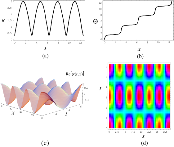
Figure 1: A plot of a MAW $\psi_{0}(x,t)$ corresponding to the equilibrium $(\frac{\pi}{2},3)$ for unperturbed system of (1.1) on the right-plane. The original system (1.1) has a MAW or QMAW $\psi_{\varepsilon}(x,t)$ such that $\big{|}\,|\psi_{0}(x,t)|-|\psi_{\varepsilon}(x,t)|\big{|}=\mathcal{O}(\varepsilon)$ for all time $t$ and the spatial domains of order $1/\varepsilon$. The parameters we take as follows: $c=1,~{}\delta=1,~{}\alpha=0.30,~{}b_{0}=-12.40,~{}b_{1}=-20.20$. (a) Spatial amplitude $R(x)$ plot; (b) Nontrivial spatial phase $\Theta(x)$ plot; (c) A plot of space-time $\mathrm{R}e[\psi(t,x)]$ ; (d) The density plot of $\mathrm{Re}[\psi(t,x)]$.

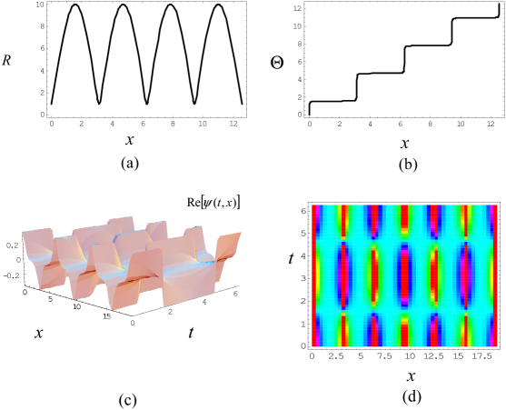
Figure 2: A plot of a MAW $\psi_{0}(x,t)$ corresponding to the equilibrium $({\pi},10)$ for unperturbed system of (1.1) on the right-plane. The original system (1.1) has a MAW or QMAW $\psi_{\varepsilon}(x,t)$ such that $\big{|}\,|\psi_{0}(x,t)|-|\psi_{\varepsilon}(x,t)|\big{|}=\mathcal{O}(\varepsilon)$ for all time $t$ and the spatial domains of order $1/\varepsilon$. The parameters we take as follows: $c=1,~{}\delta=1,~{}\alpha=0.30,~{}b_{0}=-12.40,~{}b_{1}=-20.20$. (a) Spatial amplitude $R(x)$ plot; (b) Nontrivial spatial phase $\Theta(x)$ plot; (c) A plot of space-time $\mathrm{R}e[\psi(t,x)]$ ; (d) The density plot of $\mathrm{Re}[\psi(t,x)]$.

As we know, $(\theta_{0},\rho_{0})=(k\pi+\pi/2,3.00)$ and $(\theta_{1},\rho_{1})=(k\pi,10.00)$ are hyperbolic with the eigenvalue of linearization

$$\lambda_{0}=\pm 0.95\varepsilon,~{}\lambda_{1}=\pm 15.33\varepsilon.$$

By the averaging theorem, the equilibriums can persist as the periodic orbits for the original system (3.1); in addition, these periodic orbits are also hyperbolic with respect to spatial variable $x$.

Returning to (3.1), consider its unperturbed system, and using Lemma 3.1, the periodic orbit corresponding to the equilibrium $(\theta_{0},\rho_{0})=(k\pi+\pi/2,3.00)$ is given by

$$\varphi_{0}(x)=3\sqrt{\sin^{2}x+\frac{1}{81}\cos^{2}x}.$$

Following from (2.3), we have the angle function

$$\Theta_{0}(x)=\int_{0}^{x}\frac{1}{{\varphi_{0}}^{2}(s)}\mathrm{d}s$$

with its mean value

$$\bar{\Theta}_{0} =\frac{1}{L}\int_{0}^{L}\frac{1}{{\varphi_{0}}^{2}(s)}\mathrm{d}s$$

$$=\frac{1}{\pi}\int_{0}^{\pi}\frac{1}{9(\sin^{2}x+\frac{1}{81}\cos^{2}x)}\mathrm{d}s=1.$$

We conclude that $\psi_{0}(t,x)=R_{0}(x)\exp(i[\Theta_{0}(x)-\mu t])$ is a MAW of unperturbed system (1.1), see FIG. 1. The averaging theorem implies that the MAW $\psi_{0}(t,x)$ can be continuable, i.e., there exists a MAW or QMAW $\psi_{\varepsilon}(t,x)$ for system (1.1) such that

$$\big{|}|\psi_{\varepsilon}(t,x)|-|\psi_{0}(t,x)|\big{|}=\mathcal{O}(\varepsilon),$$

for sufficiently small $\varepsilon$. We can have a similar analysis for the equilibrium $(\theta_{1},\rho_{1})=(k\pi,10.00)$, see FIG. 2.

The equilibrium $(\theta_{2},\rho_{2})=(k\pi+\pi/2,2.00)$ with the linearized eigenvalue $\lambda_{2}=\mp 6.44\varepsilon i$ also persist as periodic orbits for system (3.1). Since the equilibrium is not hyperbolic, one cannot depict the spatial dynamics of the corresponding continuable periodic orbit. This question is left open for further study.

VI Discussion and conclusion

We have given an abstract result to BECs, see Theorem 4.1. Using averaging method, we determine the location where the MAWs or QMAWs exist. Comparing the previous work, we do not restrict our discussion near the origin since the equation we have dealt with has some singularities. On the other hand, the MAWs or QMAWs studied in this paper, which have nontrivial phases, form a foliation. This is a new result in this context.

However, we can not determine the spatial dynamics of some periodic orbits corresponding to MAWs or QMAWs since the equilibriums are not hyperbolic. Maybe second or even higher-order averaging is required, and this question is left for our further study. In addition, we can not provide any information upon modulational instability in time $t$ of MAWs or QMAWs. One reason is that MAWs or QMAWs obtained in this paper are not standing waves, but the waves with nontrivial phases, which does not allow us to apply the method developed by Bronski and Raptibronski2005modulational directly. This problem may be not easy but a good topic for further study.

From the view point of a physical application, it might be reasonable to use the averaging principle to replace a mathematical model by the corresponding averaged system, to use the averaged system to make a prediction, and then to test the prediction against the results of a physical experiment. The study of this paper exactly gives a frame for application of the averaging method to BECs.

References

- (1)
- (2) M. H. Anderson, J. R. Ensher, M. R. Matthews, C. E. Wieman, E. A. Cornell, “Observation of Bose-Einstein condensation in a dilute atomic vapor”, Science 269, 198–201 (1995).
- (3) K. B. Davis, M. O. Mewes, M. R. Andrews, N. J. Van Druten, D. S. Durfee, D. M. Kurn, W. Ketterle, “Bose-Einstein condensation in a gas of sodium atoms”, Phys. Rev. Lett. 75, 3969–3973 (1995) .
- (4) K. E. Strecker, G. B. Partridge, A. G. Truscott, R. G. Hulet, “Formation and propagation of matter-wave soliton trains”, Nature 417, 150–153 (2002) .
- (5) L. Khaykovich, F. Schreck, G. Ferrari, T. Bourdel, J. Cubizolles, L. D. Carr, Y. Castin, C. Salomon, “Formation of a matter-wave bright soliton”, Science 296, 1290–1293 (2002).
- (6) S. Burger, K. Bongs, S. Dettmer, W. Ertmer, K. Sengstock, A. Sanpera, G. V. Shlyapnikov, M. Lewenstein, “Dark solitons in Bose-Einstein condensates”, Phys. Rev. Lett. 83, 5198–5201 (1999) .
- (7) J. Denschlag, D. Cassettari, J. Schmiedmayer, “Guiding neutral atoms with a wire”, Phys. Rev. Lett. 82, 2014–2017 (1999).
- (8) J. Belmonte-Beitia, P. J. Torres, “Existence of dark soliton solutions of the cubic nonlinear Schrödinger equation with periodic inhomogeneous nonlinearity”, J. Nonlinear Math. Phys. 15 65–72 (2008).
- (9) J. Belmonte-Beitia, V. M. Pérez-García, P. J. Torres, “Solitary waves for linearly coupled nonlinear Schrödinger equations with inhomogeneous coefficients”, J. Nonlinear Sci. 19, 437–451 (2009).
- (10) G. Chong, W. Hai, Q. Xie, “Spatial chaos of trapped Bose-Einstein condensate in one-dimensional weak optical lattice potential”, Chaos 14, 217–223 (2004) .
- (11) Q. Xie, W. Hai, G. Chong, “Chaotic atomic tunneling between two periodically driven Bose-Einstein condensates”, Chaos 13, 801 (2003).
- (12) M. Centurion, M. A. Porter, Y. Pu, P. G. Kevrekidis, D. J. Frantzeskakis, D. Psaltis, “Modulational instability in a layered Kerr medium: Theory and experiment”, Phys. Rev. Lett. 97, 234101 (2006).
- (13) T. Kapitula, B. Sandstede, “Stability of bright solitary-wave solutions to perturbed nonlinear Schrödinger equations”, Physica D 124, 58–103 (1998).
- (14) T. Kapitula, K. J. H. Law, P. G. Kevrekidis, “Interaction of Excited States in Two-Species Bose–Einstein Condensates: A Case Study”, SIAM J. Appl. Dyn. Syst. 9, 34–61 (2010).
- (15) C. K. Jones, R. Gardner, T. Kapitula, “Stability of travelling waves for non-convex scalar viscous conservation laws”, Commun. Pure Appl. Math. 4, 6505–526 (1993).
- (16) T. Kapitula, “Stability criterion for bright solitary waves of the perturbed cubic-quintic Schrödinger equation”, Physica D 116, 95–120 (1998).
- (17) M. Van Noort, M. A. Porter, Y. Yi, S. N. Chow, “Quasiperiodic dynamics in Bose-Einstein condensates in periodic lattices and superlattices”, J. Nonlinear Sci. 17, 59–83 (2007).
- (18) B. Deconinck, B. A. Frigyik, J. N. Kutz, “Dynamics and stability of Bose-Einstein condensates: the nonlinear Schrodinger equation with periodic potential”, J. Nonlinear Sci. 12, 169–205 (2002).
- (19) F. Dalfovo, S. Giorgini, L. P. Pitaevskii, S. Stringari, “Theory of Bose-Einstein condensation in trapped gases”, Rev. Mod. Phys. 71, 463 (1999) .
- (20) B. B. Baizakov, V. V. Konotop, M. Salerno, “Regular spatial structures in arrays of Bose–Einstein condensates induced by modulational instability”, J. Phys. B 35, 5105 (2002).
- (21) T. Köhler, “Three-body problem in a dilute Bose-Einstein condensate”, Phys. Rev. Lett. 89, 210404 (2002).
- (22) A. V. Carpentier, H. Michinel, M. I. Rodas-Verde, V. M. Pérez-García, “Analysis of an atom laser based on the spatial control of the scattering length”, Phys. Rev. A 74, 013619 (2006).
- (23) F. K. Abdullaev, J. Garnier, “Propagation of matter-wave solitons in periodic and random nonlinear potentials”, Phys. Rev. A 72, 061605 (2005).
- (24) M. A. Porter, P. G. Kevrekidis, B. A. Malomed, D. J. Frantzeskakis, “Modulated amplitude waves in collisionally inhomogeneous Bose-Einstein condensates”, Physica D 229, 104–115 (2007).
- (25) C. H. Tsang, B. A. Malomed and K. W. Chow, “Exact solutions for periodic and solitary matter waves in nonlinear lattices”, Discrete Contin. Dyn. Syst. 4, 1299-1325 (2011).
- (26) Y. V. Kartashov, B. A. Malomed and L. Torner, “Solitons in nonlinear lattices”, Rev. Mod. Phys. 83, 247–298 (2011).
- (27) B. P. Anderson, M. A. Kasevich, “Macroscopic quantum interference from atomic tunnel arrays”, Science 282, 1686 (1998) .
- (28) E. W. Hagley, L. Deng, M. Kozuma, J. Wen, K. Helmerson, S. L. Rolston, W. D. Phillips, “A well-collimated quasi-continuous atom laser”, Science 283, 1706 (1999).
- (29) J. C. Bronski, L. D. Carr, B. Deconinck, J. N. Kutz, “Bose-Einstein condensates in standing waves: The cubic nonlinear Schrödinger equation with a periodic potential”, Phys. Rev. Lett. 86, 1402–1405 (2001).
- (30) D. I. Choi, Q. Niu, “Bose-Einstein condensates in an optical lattice”, Phys. Rev. Lett. 82, 2022–2025 (1999).
- (31) A. Trombettoni, A. Smerzi, “Discrete solitons and breathers with dilute Bose-Einstein condensates”, Phys. Rev. Lett. 86, 2353–2356 (2001).
- (32) M. A. Porter, P. Cvitanović, “Modulated amplitude waves in Bose-Einstein condensates”, Phys. Rev. E 69, 047201 (2004) .
- (33) M. A. Porter, P. Cvitanovic, “A perturbative analysis of modulated amplitude waves in Bose-Einstein condensates”, Chaos 14, 739–755 (2004).
- (34) M. A. Porter, M. Chugunova, D. E. Pelinovsky, “Feshbach resonance management of Bose-Einstein condensates in optical lattices”, Phys. Rev. E 74, 036610 (2006).
- (35) M. A. Porter, P. G. Kevrekidis, B. A. Malomed, “Resonant and non-resonant modulated amplitude waves for binary Bose-Einstein condensates in optical lattices”, Physica D 196, 106–123 (2004).
- (36) V. Chua, M. Porter, “Spatial Resonance Overlap in Bose-Einstein Condensates in Superlattice Potentials”, Int. J. Bifurcation Chaos 16, 945–959 (2006).
- (37) M. A. Porter, P. G. Kevrekidis, “Bose-Einstein Condensates in Superlattices”, SIAM J. Appl. Dyn. Syst. 4, 783–807 (2005).
- (38) W. Hai, C. Lee, G. Chong, “Propagation and breathing of matter–wave-packet trains”, Phys. Rev. A 70, 053621 (2004).
- (39) N. A. Kostov, V. Z. Enol’skii, V. S. Gerdjikov, V. V. Konotop, M. Salerno, “Two-component Bose-Einstein condensates in periodic potential”, Phys. Rev. E 70, 056617 (2004).
- (40) L. D. Carr, J. N. Kutz, W. P. Reinhardt, “Stability of stationary states in the cubic nonlinear Schrödinger equation: applications to the Bose-Einstein condensate”, Phys. Rev. E 63, 066604 (2001).
- (41) N. N. Bogoliubov, Y. A. Mitropolsky, Asymptotic Methods in the Theory of Nonlinear Oscillations, Gordon and Breach, New York, 1961.
- (42) J. A. Sanders, F. Verhulst, J. A. Murdock, Averaging methods in nonlinear dynamical systems, Springer Verlag, 2007.
- (43) J. Guckenheimer, P. Holmes, Nonlinear oscillations, dynamical systems and bifurcations of vector fields, Springer-Verlag, 1983.
- (44) J. Ellison, H. Shih, The method of averaging in beam dynamics, AIP Conference Proceedings, 1995.
- (45) L. Brusch, M. G. Zimmermann, M. Van Hecke, M. Bär, A. Torcini, “Modulated amplitude waves and the transition from phase to defect chaos”, Phys. Rev. Lett. 85, 86–89 (2000).
- (46) L. Brusch, A. Torcini, M. Van Hecke, M. G. Zimmermann, M. Bär, “Modulated amplitude waves and defect formation in the one-dimensional complex Ginzburg-Landau equation”, Physica D 160, 127–148 (2001).
- (47) N. Berglund, Perturbation Theory of Dynamical Systems, Citeseer, 2001.
- (48) V. V. Konotop and M. Salerno, “Modulational instability in Bose-Einstein condensates in optical lattices”, Phys. Rev. A 65, 021602 (2002).
- (49) Z. Rapti, G. Theocharis, P. G. Kevrekidis, D. J. Frantzeskakis and B. A. Malomed, “Modulational Instability in Bose-Einstein Condensates under Feshbach Resonance Management”, Phys. Scr., 107, 27–31 (2004).
- (50) H. He, A. Arraf, C. M. de Sterke, P. D. Drummond and B. A. Malomed, “Theory of modulational instability in Bragg gratings with quadratic nonlinearity”, Phys. Rev. E, 59, 6064-6078 (1999).
- (51) Z. H. Musslimani and B. A. Malomed, “Modulational instability in bulk dispersive quadratically nonlinear media”, Physica D, 123, 235-243 (1998).
- (52) J. C. Bronski and Z. Rapti, “Modulational instability for nonlinear Schrödinger equations with a periodic potential”, Dyn. Partial Differ. Equ., 2, 335–355 (2005).
- (53)