Statistical properties of $r$-adic processes and their connections to families of popular fractal curves

Abstract

Results concerning the statists of $r$-adic processes and their fractal properties are reviewed. The connection between singular eigenstates of the statistical evolution of such processes and popular fractal curves is emphasized.

,

In memory of our friend and colleague Shuichi Tasaki whose untimely death cut short a remarkable scientific career

Among the many important scientific achievements of Shuichi Tasaki were his contributions to the statistical properties of piecewise linear maps and the characterization of their eigenstates. In particular his work was key to understanding the role played by singular measures in the statistical evolution of chaotic maps and its connection to the mathematics of fractals [1, 2]. This field, which attracted much attention in the non-equilibrium statistical physics community in the mid-1990’s [3, 4], had been popular among many Japanese mathematicians, in particular early in Tasaki’s scientific career [5]. In this respect, it is perhaps not surprising that one of Tasaki’s favorite examples of fractals, which helped understand how the non-equilibrium states of volume-preserving strongly chaotic systems acquire fractal properties [6], was actually introduced by Teiji Takagi [7], the founder of the school of modern mathematics in Japan, who, more than a century ago, had proposed it as a simple example of a continuous but nowhere differentiable function.

It is the purpose of this article to review some of Tasaki’s contributions to this field, and draw observations which aim to underline the similarities between the so-called hydrodynamic modes of diffusion of simple model systems and some popular fractals, which include the von Koch and Levy curves.

1 Singular measures of dyadic processes

The statistical properties of coin tosses are full of mathematical wonders and Shuichi Tasaki was well aware of it. Thus assume a fair coin tossing game and a sequence $\{\omega_{1},\dots,\omega_{k}\}$ of $k$ binary digits, $\omega_{i}\in\{0,1\}$, $i=1,\dots,k$, where say the symbol $0$ stands for heads and $1$ for tails. The probability measure which assigns probability $1/2$ to every symbol irrespective of which of heads or tails came at the previous toss is invariant under such a process, which in particular is to say that every set of $k$ binary digits has the same measure $1/2^{k}$. No surprise there.

Consider however an arbitrary number $p$, $0<p<1$, and let $\mu_{p}$ denote the probability measure which assigns measure $p$ to heads and $1-p$ to tails. This measure is itself invariant under fair coin tossings [8].

The reason is simply that the set $\{\omega_{1},\dots,\omega_{k}\}$ is the union of the two disjoint sets of length $k+1$,

$$\{0,\omega_{1},\dots,\omega_{k}\}\cup\{1,\omega_{1},\dots,\omega_{k}\}.$$ (1.1)

Since $\mu_{p}(\{0,\omega_{1},\dots,\omega_{k}\})=p\mu_{p}(\{\omega_{1},\dots,\omega_{k}\})$ and $\mu_{p}(\{1,\omega_{1},\dots,\omega_{k}\})=(1-p)\mu_{p}(\{\omega_{1},\dots,\omega_{k}\})$, we have that the probability measure of the left and right hand sides of equation (1.1) is the same, irrespective of the choice of the value $p$. We might say, in other words, that $\mu_{p}$ is as good an invariant measure as the uniform measure $\mu_{1/2}$ is.

There is however an essential difference here, which is that $\mu_{1/2}$ is the natural invariant measure for the fair coin tossings. For $p\neq 1/2$, $\mu_{p}$ is in fact a singular measure, which can be thought of as a singular Lebesgue function [9]. Using the isomorphism between fair coin tossings and the angle-doubling map, $x\mapsto 2x(\mathrm{mod}\,1)$, it is a simple exercise to identify $\mu_{p}$ with the measure lifted on the corresponding cylinder sets of the unit interval, whose cumulant $\mu_{p}([0,x])$ is the unique function $f_{p}(x)$ satisfying

$$f_{p}(x)=\left\{\begin{array}[]{l@{\quad}l}pf_{p}(2x),&0\leq x<1/2,\\ (1-p)f_{p}(2x-1)+p,&1/2\leq x<1.\end{array}\right.$$ (1.2)

Except for $p=1/2$, for which $f_{1/2}(x)=x$, $f_{p}$ is strictly increasing and continuous, but has zero derivatives almost everywhere with respect to the Lebesgue measure [10]. A specific example is shown in figure 1.

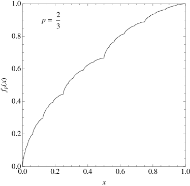
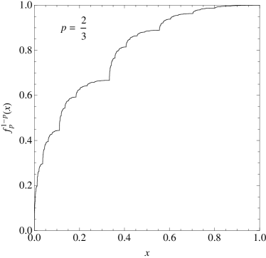
Figure 1: (a) Lebesgue’s singular function $f_{p}$, equation (1.2), and (b) $f_{p}^{(1-p)}$, equation (1.3), both with $p=2/3$. Here and below, unless otherwise stated, the curves are computed over $2^{14}$ points.

Notice however that $\mu_{p}$ is in fact the natural invariant measure of the biased coin tossing which gives probability $p$ to heads and $1-p$ to tails. Its cumulant corresponds to a uniform measure, which can be identified as the solution of the more general functional equation

$$f^{(q)}_{p}(x)=\left\{\begin{array}[]{l@{\quad}l}pf^{(q)}_{p}(\frac{x}{q}),&0\leq x<q,\\ (1-p)f^{(q)}_{p}(\frac{x-q}{1-q})+p,&q\leq x<1.\end{array}\right.$$ (1.3)

Setting $q=p$ indeed yields $f^{(p)}_{p}(x)=x$. On the other hand, the function $f_{p}^{(1-p)}$, illustrated in figure 1, is of the Lebesgue singular type and arises as the cumulant of the natural invariant measure of a dissipative baker map, projected along the contracting direction [9].

2 Complex-valued measures of dyadic processes

Though equation (1.2) is a functional equation characterizing a probability measure, it is not in itself restricted to real values of the parameter $p$. The uniqueness of its solutions is indeed warranted for every complex parameter $p$ such that $|p|,|1-p|<1$ [11, 12]. In such cases the solutions of equation (1.2) are self-similar sets on the complex plane and it is a simple calculation to show that their Hausdorff dimension is the solution $d_{\mathrm{H}}$ of the following equation [13],

$$|p|^{d_{\mathrm{H}}}+|1-p|^{d_{\mathrm{H}}}=1.$$ (2.1)

A graphical representation of its solution is shown in figure 2.

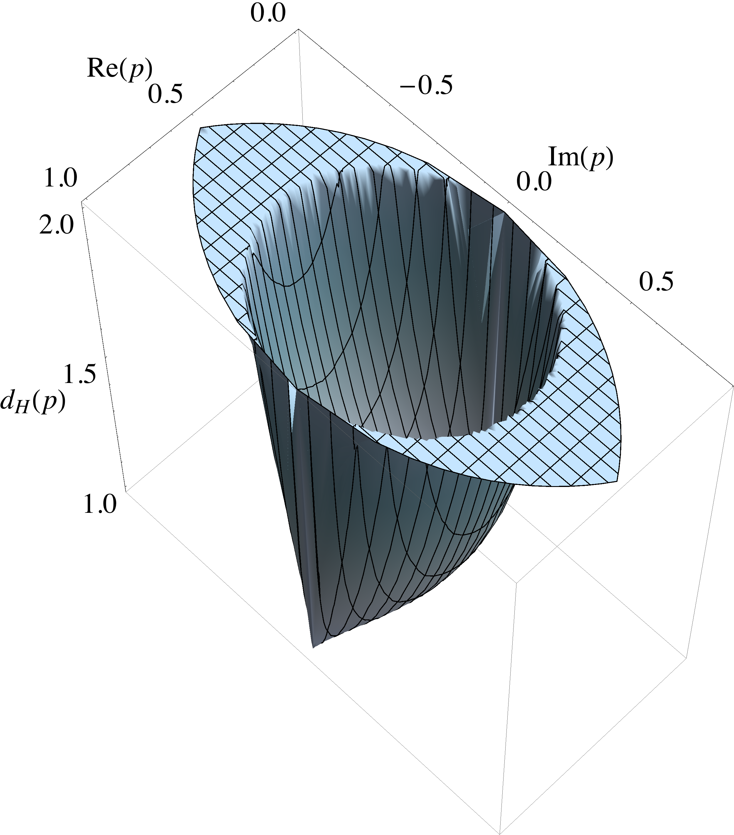
Figure 2: Hausdorff dimension (2.1) of the curves $f_{p}$ defined through equation (1.2).

Note in particular that the parameter values $p=1/2(1+e^{\imath\varphi})$, $0\leq\varphi<2\pi$, define a circle of complex parameters such that the dimension (2.1) is equal to $d_{\mathrm{H}}=2$. Curves with parameters whose values lie inside that circle have Hausdorff dimension between $1$ and $2$. Curves with parameters which verify the conditions $|p|<1$ and $|1-p|<1$, but which lie outside that circle have Hausdorff dimension $2$ [12]

As shown by Tasaki and collaborators [2], the functions $f_{p}$ with complex parameter

$$p(k)=\frac{e^{\imath k}}{2\cos k}=\frac{1}{2}\left(1+\imath\tan k\right),$$ (2.2)

with $k$ a real number such that $|k|<\pi/3$, occur as representations of the left eigenvectors of the Frobenius-Perron operator of an expanding piecewise linear map of the real line related to the angle-doubling map.

The same curves also occur as special cases of hydrodynamic modes of diffusion, associated with multi-baker maps on a ring [14], where $k$ is the associated wavenumber. The dynamics is defined according to

$$(n,x,y)\mapsto\left\{\begin{array}[]{l@{\quad}l}(n-1,2x,\frac{y}{2}),&0\leq x<1/2,\\ (n+1,2x-1,\frac{y+1}{2}),&1/2\leq x<1,\end{array}\right.$$ (2.3)

where $n=0,\dots,N-1$ and $n\pm 1$ are understood to be taken modulo $N$. Given an initial distribution, the relaxation of statistical ensembles to the uniform equilibrium measure takes place exponentially fast at rate $\sim N^{-2}$ and is best characterized in terms of the cumulant measure $\mu_{t}(n,[0,1],[0,y])$ of phase points $(n,\tilde{x},\tilde{y})$, with $0\leq\tilde{x}<1$ and $0\leq\tilde{y}<y$, after $t$ iterations:

$$\mu_{t}(n,[0,1],[0,y])=\sum_{k}a_{k}\cos^{t}(k)F_{k}(y)e^{\imath kn},$$ (2.4)

where $k=2\pi m/N$, $m=0,\dots,N-1$ are the wavenumbers, the coefficients $a_{k}$ are set by the initial distribution, and $F_{k}$ are solutions of the system of equations (1.2) with the choice of parameter (2.2), $F_{k}(x)\equiv f_{p(k)}(x)$, viz.

$$F_{k}(x)=\left\{\begin{array}[]{l@{\quad}l}\frac{e^{\imath k}}{2\cos k}F_{k}(2x),&0\leq x<1/2,\\ \frac{e^{-\imath k}}{2\cos k}F_{k}(2x-1)+\frac{e^{\imath k}}{2\cos k},&1/2\leq x<1.\end{array}\right.$$ (2.5)

The dimension (2.1) of these curves can be computed explicitly [2]:

$$d_{\mathrm{H}}(k)=\frac{\log 2}{\log(2|\cos k|)}.$$ (2.6)

In particular, for $k=\pi/4$, we obtain a curve of Hausdorff dimension $d_{\mathrm{H}}(\pi/4)=2$ which covers positive areas of the plane and corresponds to the Levy dragon [15]. Another remarkable value of the parameter is $k=\pi/6$, for which we have the dimension $d_{\mathrm{H}}(\pi/6)=\log 4/\log 3$. These two curves are displayed in figure 3.

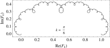
(a) Fractal curve with dimension $\log 4/\log 3$

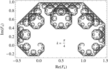
(b) Levy dragon with dimension $2$

Figure 3: Specific examples of hydrodynamic modes for the dyadic process defined by the functional equations (2.5).

In the context of hydrodynamic modes of diffusion [16], the complex curves defined by equation (1.2) acquire a clear physical meaning , which comes about when the parameter $k$ in (2.2) is small: $|k|\ll 1$. The Hausdorff dimension (2.6) then becomes [14]

$$d_{\mathrm{H}}(k)=1+\frac{k^{2}}{2\log 2}+\mathcal{O}(k^{4}),$$ (2.7)

which provides a relation between the Hausdorff dimension of the hydrodynamic modes, the diffusion coefficient of the process and the positive Lyapunov exponent of the underlying dynamics (2.3). Furthermore, considering the functional equation (2.5), we obtain the equivalent of a gradient expansion for $F_{k}$ [17],

$$F_{k}(x)=x+\imath kT(x)+\mathcal{O}(k^{2}),$$ (2.8)

where $T(x)$ is the Takagi function [7], which can be defined through the functional equation:

$$T(x)=\left\{\begin{array}[]{l@{\quad}l}x+\frac{1}{2}T(2x),&0\leq x<1/2,\\ 1-x+\frac{1}{2}T(2x-1),&1/2\leq x<1.\end{array}\right.$$ (2.9)

See figure 4.

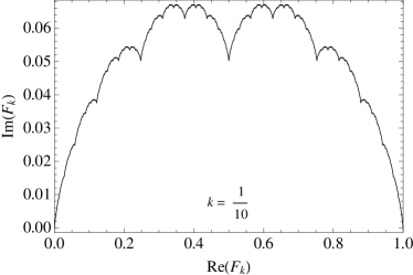
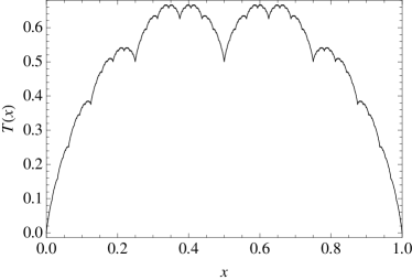
Figure 4: The graph of the function $F_{k}$, equation (2.5), with $k=1/10$ (a), approaches that of the Takagi function (2.9) (b).

The result (2.8) should be compared with that of Hata and Yamaguti [18, 19], who recover the Takagi function as the derivative of the curves $f_{p}$, equation (1.2), with respect to their parameter, $T(x)=\partial f_{p}(x)/\partial p|_{p=1/2}$.

3 Levy, von Koch and Heighway curves

The Levy dragon shown in figure 3(b) is but one example in a long list of popular fractal curves which are most often defined recursively through iterated function systems [20] or using $L$-systems [21]. The von Koch curve [22] and the Heighway dragon, popularized in Martin Gardner’s Mathematical games [23], are two other similar examples. In analogy with equation (1.2), it is simple to identify linear contractions which generate these sets [24, 25].

The solutions of equation (1.2) with complex parameters produce a family of curves somewhat similar to the Levy dragon. Looking at the iterative construction of these solutions, we start from the initial line segment joining $F_{k}(0)=0$ and $F_{k}(1)=1$ and obtain $F_{k}(1/2)=e^{\imath k}/(2\cos k)$. At the next iteration, we add the two points $F_{k}(1/4)$ and $F_{k}(3/4)$. The result on the complex plane is a collection of two isosceles triangles whose long edges correspond to the two smaller edges of the triangle formed by the three initial points $F_{k}(0)$, $F_{k}(1/2)$ and $F_{k}(1)$. The next iteration produces four smaller isosceles triangles which are stacked upon the small edges of the two existing ones. See figure 5.

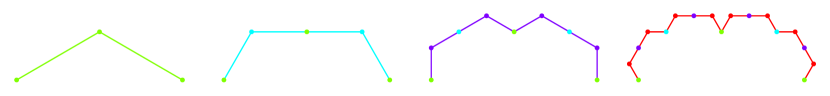
Figure 5: Comparison between the first few steps of the iterative constructions of (a) the Levy curve and (b) the von Koch curve.

A similar construction, which consists of stacking up the triangles alternatively upwards and downwards from one iteration to the next, as shown in figure 5, produces curves similar to the von Koch curve. They are most easily obtained as the self-similar sets associated with a linear contraction similar to equation (1.2), but that further involves complex conjugation:

$$g_{p}(x)=\left\{\begin{array}[]{l@{\quad}l}pg_{p}^{*}(2x),&0\leq x<1/2,\\ (1-p)g_{p}^{*}(2x-1)+p,&1/2\leq x<1,\end{array}\right.$$ (3.1)

where ^∗ denotes the complex conjugation. Equations (1.2) and (3.1) share the same real solutions but have different sets of solutions for complex parameter values. Nonetheless they share the same Hausdorff dimension (2.1). As pointed out by de Rham [12], the choice $p=1/2(1+\imath/\sqrt{3})$ produces the von Koch curve.

Taking the parameter $p$ as defined by equation (2.2), we write $G_{k}(x)\equiv g_{p(k)}(x)$, for which we have the functional equation:

$$G_{k}(x)=\left\{\begin{array}[]{l@{\quad}l}\frac{e^{\imath k}}{2\cos k}G_{k}^{*}(2x),&0\leq x<1/2,\\ \frac{e^{-\imath k}}{2\cos k}G_{k}^{*}(2x-1)+\frac{e^{\imath k}}{2\cos k)},&1/2\leq x<1.\end{array}\right.$$ (3.2)

As illustrated in figure 6, the choice of parameter $k=\pi/6$ corresponds to the von Koch curve. For $k=\pi/4$ we obtain a Peano-like curve.

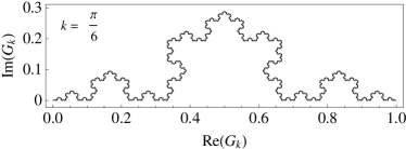
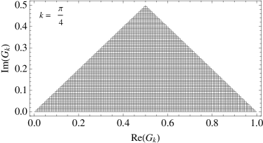
Figure 6: Specific examples of solutions of the functional equation (3.2) yield (a) the von Koch curve and (b) a Peano-type curve.

As such, the functional equation (3.2) is different from equation (2.5) so its solutions do not correspond to hydrodynamic modes of the dyadic multi-baker map (2.3). It is however straightforward to see that they are the hydrodynamic modes associated with the four-adic map,

$$(n,x,y)\mapsto\left\{\begin{array}[]{l@{\quad}l}(n,4x,\frac{y}{4}),&0\leq x<1/4,\\ (n-1,4x-1,\frac{y+1}{4}),&1/4\leq x<1/2,\\ (n+1,4x-2,\frac{y+2}{4}),&1/2\leq x<3/4,\\ (n,4x-3,\frac{y+3}{4}),&3/4\leq x<1,\end{array}\right.$$ (3.3)

with wavenumbers halved. Note that the iterative construction of the von Koch curve using a four-adic process amounts to skipping every odd step in the dyadic-based iterative construction shown in figure 5. The former is often preferred over the latter in the literature, see for instance [26], even though the dyadic representation based on equation (3.2) is indeed the most compact.

The Heighway dragon and related curves can also be obtained through functional equations similar to equation (1.2). They are based upon iterative constructions which combine both upwards and downwards triangles, as shown in figure 7.

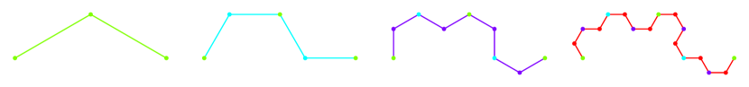
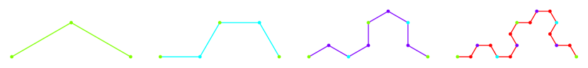
Figure 7: First few steps of the iterative constructions of asymmetric curves similar to the the Levy and von Koch constructions of figure 5.

The Heighway dragon is in fact a particular case of a hydrodynamic mode of a dyadic map similar to the multibaker map (2.3), where the angle-doubling map is replaced by the tent map $x\mapsto 2x$ if $0\leq x<1/2$ and $2(1-x)$ if $1/2\leq x<1$, namely

$$(n,x,y)\mapsto\left\{\begin{array}[]{l@{\quad}l}(n-1,1-2x,\frac{y}{2}),&0\leq x<1/2,\\ (n+1,2x-1,1-\frac{y}{2}),&1/2\leq x<1.\end{array}\right.$$ (3.4)

Note that the tent map here appears upside down along the expanding direction. This choice of combination of maps along the $x$ and $y$ coordinates is taken so the map has the property of being time reversal symmetric under the induction $(n,x,y)\mapsto(n,1-y,1-x)$, which is also the case of the multi-baker map (2.3). Another such map, very similar to equation (3.4), is

$$(n,x,y)\mapsto\left\{\begin{array}[]{l@{\quad}l}(n-1,2x,\frac{1-y}{2}),&0\leq x<1/2,\\ (n+1,2(1-x),\frac{y+1}{2}),&1/2\leq x<1.\end{array}\right.$$ (3.5)

Here the usual tent map acts along the expanding direction. For the sake of our argument however, we prefer using (3.4) since the tent map appears along the contracting direction under the time-evolution of phase-space densities.

Using, for the evolution of statistical ensembles under (3.4), an expansion similar to equation (2.4), we identify the modes

$$P_{k}(x)=\left\{\begin{array}[]{l@{\quad}l}\frac{e^{\imath k}}{2\cos k}P_{k}(2x),&0\leq x<1/2,\\ 1-\frac{e^{-\imath k}}{2\cos k}P_{k}(2(1-x)),&1/2\leq x<1.\end{array}\right.$$ (3.6)

The value $k=\pi/4$ yields the Heighway dragon, as shown in figure 8. The map (3.5) produces modes which can be obtained from equation (3.6) by a simple symmetry.

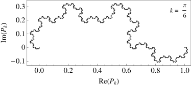
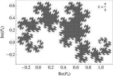
Figure 8: Examples of different solutions of equation (3.6) with (a) $k=\pi/6$ and (b) $k=\pi/4$. The latter is knwon as the Heighway dragon

Finally, by analogy with equation (3.2), we obtain another set of associated fractals by complex conjugating the function on the right-hand side of the functional equation,

$$Q_{k}(x)=\left\{\begin{array}[]{l@{\quad}l}\frac{e^{\imath k}}{2\cos k}Q^{*}_{k}(2x),&0\leq x<1/2,\\ 1-\frac{e^{-\imath k}}{2\cos k}Q^{*}_{k}(2(1-x)),&1/2\leq x<1.\end{array}\right.$$ (3.7)

Examples of solutions are shown in figure 9. Here again these curves can be identified as the hydrodynamic modes of a four-adic map.

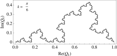
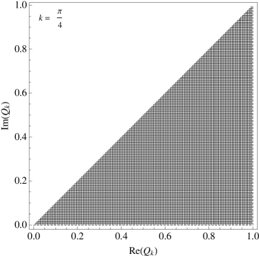
Figure 9: Two different solutions of equation (3.7) with (a) $k=\pi/6$ and (b) $k=\pi/4$, which is another example of Peano-type curve.

4 Complex measures of $r$-adic processes

The above considerations are not limited to dyadic processes. Consider for instance the iterated systems shown in figure 10

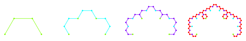
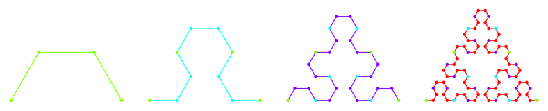
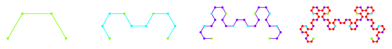
Figure 10: These three examples of iterative constructions of fractal curves are based upon triadic processes which can be conveniently written under the form of functional equation systems (4.4)-(4.12).

The functional equations whose solutions reproduce these familiar curves are based upon triadic processes:

$$U_{k}(x)=\left\{\begin{array}[]{l@{\quad}l}\frac{e^{\imath k}}{1+2\cos k}U_{k}(3x),&0\leq x<1/3,\\ \frac{e^{\imath k}}{1+2\cos k}+\frac{1}{1+2\cos k}U_{k}(3x-1),&1/3\leq x<2/3,\\ \frac{e^{\imath k}+1}{1+2\cos k}+\frac{e^{-\imath k}}{1+2\cos k}U_{k}(3x-2),&2/3\leq x<1,\end{array}\right.$$ (4.4)

$$V_{k}(x)=\left\{\begin{array}[]{l@{\quad}l}\frac{e^{\imath k}}{1+2\cos k}V^{*}_{k}(3x),&0\leq x<1/3,\\ \frac{e^{\imath k}}{1+2\cos k}+\frac{1}{1+2\cos k}V_{k}(3x-1),&1/3\leq x<2/3,\\ \frac{e^{\imath k}+1}{1+2\cos k}+\frac{e^{-\imath k}}{1+2\cos k}V^{*}_{k}(3x-2),&2/3\leq x<1,\end{array}\right.$$ (4.8)

$$W_{k}(x)=\left\{\begin{array}[]{l@{\quad}l}\frac{e^{\imath k}}{1+2\cos k}W_{k}(3x),&0\leq x<1/3,\\ \frac{e^{\imath k}}{1+2\cos k}+\frac{1}{1+2\cos k}W^{*}_{k}(3x-1),&1/3\leq x<2/3,\\ \frac{e^{\imath k}+1}{1+2\cos k}+\frac{e^{-\imath k}}{1+2\cos k}W_{k}(3x-2),&2/3\leq x<1,\end{array}\right.$$ (4.12)

Equation (4.4) defines the hydrodynamic modes of diffusion of the triadic multi-baker map [14]. Equations (4.8) and (4.12) correspond, on the other hand, to the hydrodynamic modes of nine-adic multi-baker maps associated with random walks with assigned probabilities $1/9$ to jump by two units to the left or right, $2/9$ by a single unit, and $1/3$ to remain put. Notice in particular that equation (4.8) produces the Sierpinski gasket [27] for $k=\pi/3$, as shown in figure 11.

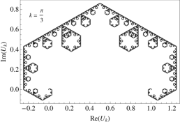
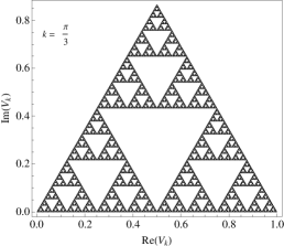
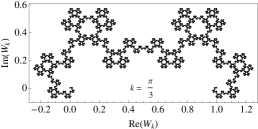
Figure 11: Examples of different solutions of equations (a) (4.4), (b) (4.8), and (c) (4.12), with $k=\pi/3$, here computed over $3^{9}$ points.

Further examples of piecewise linear maps and their associated eigenstates can be found in [28].

5 Concluding remarks

In [6], Tasaki and Gaspard showed that the Takagi function describes the non-equilibrium stationary state of a multi-baker map, and used its properties to show that this system obeys Fick’s law, which provides an expression of the mass current as minus the product of the mass density gradient and diffusion coefficient. This result thus provided a derivation of a phenomenological law of thermodynamics in terms of the phase-space dynamics of the model, which subsequently lead Gaspard to identify the fractality of the non-equilibrium stationary states as the source of entropy production [29]. A recent survey of these results with further extensions can be found in [30].

In this paper we have presented some of these results in the more general context of fractal curves and self-similar sets defined by linear contractions, and emphasized their connections with the statistical properties of maps that generate the associated functional equations. Shuichi Tasaki contributed in important ways to our understanding the connection between singular functions and the statistical properties of $r$-adic maps. We are deeply saddened that we are not able to talk to Shuichi about the excursion into the world of fractals described here. We know that we would have learned still more about them, and benefited from his careful and clear explanations.

References

References

- [1] I Antoniou and S Tasaki. Generalized spectral decomposition of the -adic baker’s transformation and intrinsic irreversibility. Physica A, 190 303, 1992.
- [2] S Tasaki, I Antoniou, and Z Suchanecki. Deterministic diffusion, de rham equation and fractal eigenvectors. Phys Lett A, 179 97, 1993.
- [3] P Gaspard. Chaos, Scattering and Statistical Mechanics. (Cambridge University Press, Cambridge, 1998).
- [4] J R Dorfman. An Introduction to Chaos in Nonequilibrium Statistical Mechanics. (Cambridge University Press, Cambridge, 1999).
- [5] M Hata. Fractals in mathematics. Patterns and Waves-Qualitative Analysis of Nonlinear Differential Equations, 259, 1986.
- [6] S Tasaki and P Gaspard. Fick’s law and fractality of nonequilibrium stationary states in a reversible multibaker map. J Stat Phys, 81 935, 1995.
- [7] T Takagi. A simple example of a continuous function without derivative. Proc Phys Math Soc Jpn, 1 176, 1903.
- [8] J-P Eckmann and D Ruelle. Ergodic theory of chaos and strange attractors. Rev Mod Phys, 57 617, 1985.
- [9] S Tasaki, T Gilbert, and J R Dorfman. An analytical construction of the SRB measures for baker-type maps. Chaos, 8 424, 1998.
- [10] P Billingsley. Ergodic Theory and Information. (Wiley, New York, 1965).
- [11] G de Rham. Sur un exemple de fonction continue sans dérivée. Enseign Math, 3 71, 1957.
- [12] G de Rham. Sur quelques courbes définies par des équations fonctionnelles. Rend Semin Mat Torino, 16 101, 1957.
- [13] S Tasaki, I Antoniou, and Z Suchanecki. Spectral decomposition and fractal eigenvectors for a class of piecewise linear maps. Chaos Solitons Fractals, 4 227, 1994.
- [14] T Gilbert, J R Dorfman, and P Gaspard. Fractal dimensions of the hydrodynamic modes of diffusion. Nonlinearity, 14 339, 2001.
- [15] P Lévy. Les courbes planes ou gauches et les surfaces composées de parties semblables au tout. J Ecole Polytechn, 3 227, 1938.
- [16] P Gaspard, I Claus, T Gilbert, and J R Dorfman. Fractality of the hydrodynamic modes of diffusion. Phys Rev Lett, 86 1506, 2001.
- [17] T Gilbert, J R Dorfman, and P Gaspard. Entropy production, fractals, and relaxation to equilibrium. Phys Rev Lett, 85 1606, 2000.
- [18] M Yamaguti and M Hata. Weierstrass’s function and chaos. Hokkaido Math J, 12 333, 1983.
- [19] M Hata and M Yamaguti. The takagi function and its generalization. Jpn J Ind Appl Math, 1 183, 1984.
- [20] G A Edgar. Measure, topology, and fractal geometry. (Springer, Berlin, 2008).
- [21] P Prusinkiewicz. Graphical applications of L-systems. Proceedings of Graphics Interface ’86 / Vision Interface ’86 247, 1986.
- [22] H von Koch. Sur une courbe continue sans tangente, obtenue par une construction géométrique élémentaire. Ark Mat Astr Fys, 1 681, 1904.
- [23] M Gardner. Mathematical Magic Show. (MAA Spectrum, Mathematical Association of America, Washington DC, 1989).
- [24] M Hata. On the structure of self-similar sets. Jpn J Ind App Math, 2 381, 1985.
- [25] M Yamaguti, M Hata, and J Kigami. Mathematics of fractals. Translations of Mathematical Monographs, 167, (American Mathematical Society, Providence RI, 1997).
- [26] W Benenson, J W Harris, H Stocker, and H Lutz. Handbook of Physics. (Springer-Verlag, New York, 2002).
- [27] W Sierpinski. Sur une courbe cantorienne dont tout point est un point de ramification. C R Acad Sci Paris, 160 302, 1915.
- [28] D J Driebe. Fully chaotic maps and broken time symmetry. (Kluwer Academic Publishers, Dordrecht, 1999).
- [29] P Gaspard. Entropy production in open volume-preserving systems. J Stat Phys, 88 1215, 1997.
- [30] F Barra, P Gaspard, and T Gilbert. Fractality of the nonequilibrium stationary states of open volume-preserving systems. I. tagged particle diffusion. Phys Rev E, 80 021126, 2009.