Accumulation of beneficial mutations in one dimension

Abstract

When beneficial mutations are relatively common, competition between multiple unfixed mutations can reduce the rate of fixation in well-mixed asexual populations. We introduce a one-dimensional model with a steady accumulation of beneficial mutations. We find a transition between periodic selection and multiple-mutation regimes. In the multiple-mutation regime, the increase of fitness along the lattice bears a striking similarity to surface growth phenomena, with power law growth and saturation of the interface width. We also find significant differences compared to the well-mixed model. In our lattice model, the transition between regimes happens at a much lower mutation rate due to slower fixation times in one dimension. Also the rate of fixation is reduced with increasing mutation rate due to the more intense competition, and it saturates with large population size.

I Introduction

In population genetics, the study of the rate at which mutations are generated and incorporated into populations has been largely a theoretical activity due to the difficulty of measuring changes in organisms over many generations. The simplest case is called periodic selection, when beneficial mutations are rare such that each mutation has ample time to spread to the whole population before the next mutation arrives. We assume conditions such that harmful mutations die out quickly and survive at a negligible rate, so we only consider beneficial mutations. In this regime the rate of fixation is limited by the rate at which mutations appear in the population.

However, recent experiments in microbes suggest that beneficial mutations may be more common than previously thought (Sniegowski and Gerrish, 2010). The competition between multiple unfixed beneficial mutations is termed clonal interference (Gerrish and Lenski, 1998) (Fig 1a). In this picture some good mutations must be wasted because only one of them ultimately fixates, which reduces the average probability of fixation, and reduces the rate of fixation. Larger mutations are more likely to survive competition, eliminating mutations of weak effect, and biasing the distribution of fixated mutational effects. Sexual organisms may alleviate this problem by recombining mutations, known as the Fisher-Muller hypothesis (Muller, 1932; Fisher, 1930), An analogue of clonal interference when mutations are linked is known as the Hill-Robertson effect (Hill and Robertson, 1966; Barton, 1995). Since our goal is to focus on the effects of spatial structure, we avoid complications associated with sexual reproduction and study only asexual organisms.

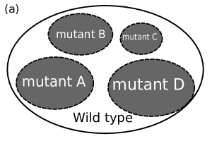
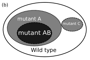
Figure 1: All mutations shown are assumed to be beneficial compared to the wild-type. (a) Clonal interference: mutation A has to compete with mutations B, C, and D, reducing its chances of fixation compared to the case when there is only one mutation. If mutation A fixates, mutations B, C, and D are “wasted”, slowing down the rate of fixation . (b) Multiple-mutation effect: Mutation AB arises in a population with Mutation A, increasing mutation A’s chances of fixation.

The original clonal interference model neglected the possibility that an individual may acquire multiple beneficial mutations. Assuming mutations are additive, an additional mutation improves the chances of fixation of the first mutation instead of suppressing it, and the simultaneous fixation of multiple mutations becomes possible (Fig 1b) (Kim and Orr, 2005; Barrett et al., 2006; Desai and Fisher, 2007; Desai et al., 2007; Fogle et al., 2008). Current research concerns a complete description that takes into account both aspects (Hallatschek, 2010) (for a review see (Sniegowski and Gerrish, 2010; Park et al., 2010)). Generally, research in clonal interference and multiple mutations find the rate of adaptation, or speed of evolution, to be slower than periodic selection. Clonal interference analysis finds fixation to occur in isolated instances, as in the periodic selection regime. In contrast, multiple mutation analysis finds fixation occurs in clusters, and because of the stacking of mutations, no mutation ever dominates the entire population. Simulation studies have found that the relative importance of either effect depends on the distribution of beneficial mutations effects (Fogle et al., 2008; Park and Krug, 2007). If the distribution has a heavy tail, and large effects are relatively common, then clonal interference can dominate. If the distribution has a sharp cutoff, and large effects are relatively rare, then effects from multiple mutations can be more important. Unfortunately, we do not know what distributions are found in nature, and it may depend on the level of adaptation to the environment (Orr, 2010; Martin and Lenormand, 2008).

In this paper we will investigate the accumulation of beneficial mutations of a population with spatial structure. While the fixation probability of a mutant on a spatially structured population is usually the same as in a well-mixed population (Maruyama, 1970; Lieberman et al., 2005), the time scales can be much slower (Chaves Filho et al., 2010; Whitlock, 2003; Habets et al., 2007). In a well-mixed population every individual competes with each other, but with spatial structure the spread of a mutant is restricted by space. Nothing happens inside a domain where the fitnesses are all the same. The only changes are at the boundaries which are defined by fitness differences. Gordo and Campos (Gordo and Campos, 2006) studied the speed of evolution on a 2D lattice. They found the speed to be slower, and the time to fixation to be longer, than in a well-mixed population, and their results were supported by experiments with bacteria (Perfeito et al., 2008). Others have studied the loss of genetic variation in 1D stepping stone models to describe the boundary of an expanding bacterial colony (Hallatschek et al., 2007; Hallatschek and Nelson, 2008, 2010; Korolev et al., 2010). Starting with multiple alleles, they found that over time the population segregates into domains of single alleles. The effects of drift and selection change significantly, since they act only on the domain boundaries. The timescale of segregation was found to be slower than in the well-mixed case (algebraic instead of exponential).

We chose to study a one-dimensional spatial structure because it is the simplest structure where we would expect the most deviation from well-mixed models. While Hallatschek and Nelson also studied the accumulation of beneficial mutations in an expanding frontier in the non-interacting regime (Hallatschek and Nelson, 2010), we will study a model where mutations are common enough to interfere with each other. In section II, we will introduce a Wright-Fisher model on a 1D lattice and study the dependence on the rate of beneficial mutations, and the size of the population. Our model has three timescales that are not well separated: selection, mutation and stochasticity (drift). Such three-timescale models are difficult to analyze analytically and we must resort to simulations for most of our insights. In section III we discuss the similarity to surface growth phenomena, and in section IV we discuss how our results remain qualitatively the same under more general conditions.

II 1-D model with mutations and selection

Our model consists of a 1-D lattice with $N$ sites and periodic boundary conditions. Unlike stepping stone models with sub-populations or demes, there is only one asexual haploid individual at every site. Time is discrete and represents each generation (parallel updates), and the total population $N$ stays constant. Each generation dies and is replaced by its offspring which inherit the fitness of their single parent. The major change from well-mixed models is that we specify a spatial neighborhood which limits where parents may have their children. For simplicity we chose the smallest possible neighborhood of size 2. An organism at site $i$ and time $t$ may have children at time $t+1$ at sites $i$ and $i+1$ when $t$ is odd and sites $i$ and $i-1$ when $t$ is even. The new generation is chosen so the number of children of each parent is proportional to its fitness relative to its neighbors’ fitness. In simulation this amounts to each child “choosing” its parent weighted by their fitnesses. For each child at site $i$, the fitness is copied from parent site $i$ with probability $f_{i}/(f_{i}+f_{i\pm 1})$ or from site $i\pm 1$ with probability $f_{i\pm 1}/(f_{i}+f_{i\pm 1})$.

Every generation, the number of mutations is determined by a Poisson random number with mean $UN$. The effect of a mutation is to increase the fitness, $f_{i}$, multiplicatively as $f^{\prime}_{i}=f_{i}(1+s)$, where $s$ is a small constant . In the multiplicative fitness model the fitness of a new mutation relative to its neighbors remains the same since common factors in the fitness drop out. The balance of mutation and selection leads to a steady state in the variance of the log fitnesses. The fitness averaged over the population, $\bar{f}(t)$ will increase exponentially as a function of time, and the speed of evolution is the rate constant defined as:

$$v=\lim_{t\rightarrow\infty}\frac{\langle\ln\bar{f}(t)\rangle}{t},$$ (1)

where brackets indicate the ensemble average. Since $s$ is constant, $v$ is related to the rate of fixation $R$, simply as $R=v/s$.

In the competing mutation regime, after an initial transient phase a progressing interface forms in log-fitness space reminiscent of surface growth phenomena (figure 2).

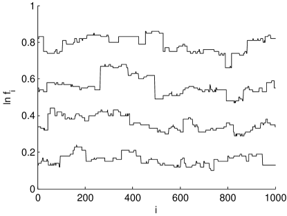
Figure 2: The logarithm of the fitness varies in spatial position. This interface moves with velocity $v$ and has a standard deviation $\sigma$. $N=1000$, $U=10^{-3}$, $s=0.01$. Shown are snapshots separated by 10000 generations

The interface of the logarithm of the fitness has a distribution that fits extremely well to a traveling Gaussian wave with a speed $v$ and a standard deviation $\sigma$. In general, these quantities depend on $U$ and $N$. The additive increases in log-fitness and spreading of mutations parallel the addition of particles and smoothing of the interface in surface growth. From the simulation it was determined that the system reaches a steady state after $\sim 100N$ generations.

As in the original multiple-mutations model, the population has a moving distribution of fitnesses with a steady width. This is in contrast to the original clonal interference model where the distribution of fitnesses varied and dropped to zero when fixation occurred.

The multiple-mutation regime occurs when the fixation time is approximately equal to or greater than the time for mutations to appear and establish themselves:

$$t_{\textrm{fix}}\gtrsim t_{\textrm{mut}}$$ (2)

The fixation probability, $\pi$, for a single mutation happens to be the same as in the well-mixed model (Lieberman et al., 2005), $\pi=2s$ for large $Ns$ and small $s$ (Kimura, 1962). The average time between fixating mutations is

$$t_{\textrm{mut}}\approx\frac{1}{2sUN}.$$ (3)

In the periodic selection regime, each mutation has time to spread to the whole population before the next mutation arrives, or $t_{\textrm{fix}}\ll t_{\textrm{mut}}$, and the rate of fixation is mutation limited:

$$R_{s}=\frac{1}{t_{\textrm{mut}}}=2sUN.$$ (4)

The transition to the multiple-mutation regime occurs when $t_{\textrm{mut}}\sim t_{\textrm{fix}}$. The fixation time for a single mutant can be formulated as a first passage problem. The fixation time is the mean time for a stochastic particle (representing the size of the mutant domain) to first reach position $N$ without ever reaching position $0$. The largest contributing term to the fixation time (when $N$ is not too small) is simply the size of the system divided by the drift velocity, or

$$t_{\textrm{fix}}=\frac{2N}{s}.$$ (5)

This is confirmed with simulations in figure 3, although some deviation is present from terms of order $s^{-2}$.

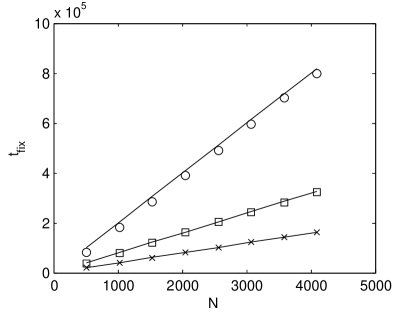
Figure 3: Fixation times were determined by planting single mutations with $s=0.01$ (circles), $s=0.025$ (squares), and $s=0.05$ (x’s), averaged over 100 fixations. Lines indicate $t_{fix}=2N/s$

The transition between the regimes is obtained by equating (3) and (5) which results in: $U_{\textrm{tr}}\sim 1/(4N^{2})$. Figure 4 shows that the fixation rate follows (4) in the periodic selection regime As $U$ approaches 1, every site receives a mutation at every generation on average, and no mutation has a relative fitness advantage. Therefore the rate of fixation approaches the neutral fixation rate, $R=U$ (figure 4a, dashed line). Between the two extremes we observe a transition.

Figure 4: (a) Fixation rate $R$ versus mutation rate $U$ with $N=512$ and $s=0.01$ averaged over $10^{3}$ fixations for the 1D model (circles) and well-mixed model (squares). The dotted line indicates the transition between the single-fixation regime and the multiple-mutation regime for the spatial model, and the dot-dashed line indicates the transition for the well-mixed wright-fisher model. The solid line is the non-interfering fixation rate (4), and the dashed line is the neutral fixation rate, $R_{n}=U$. (b) The difference between the 1D model (circles) and the well-mixed model (squares) is clearer with $R/U-1$, which approaches zero as $R$ approaches the neutral fixation rate $R_{n}=U$. As guides, the dashed and dotted lines indicate power law relations with exponents -0.25, and -0.3 respectively.

We also simulate the standard well-mixed Wright-Fisher model with constant $s$ according to (Park et al., 2010). Since the fixation time is $t_{\textrm{fix}}=2\ln(N)/s$ , the transition happens at $U\sim 1/(4N\ln N)$. Figure 4a shows that the transition happens at much higher $U$ in the well-mixed model, and the gap separating the two transitions grows with system size. The difference is more clearly seen by dividing $R$ with $U$ , shown in figure 4b. The fixation rate approaches the neutral fixation rate as a power law $\sim U^{\gamma}$, with $\gamma=0.3-0.4$

The fixation rate is always higher in the well-mixed model than in one dimension. The difference in $R$ between the models may seem small, however it is a logarithmic plot, and more importantly the difference depends on the system size $N$. Figure 5 shows that $R$ becomes independent of $N$ at large $N$, while the well-mixed model has a sub-linear dependence on $N$. The saturation of $R$ with system size is not intuitive. Mutations must either fixate or be lost, so one may write down a conservation relation:

$$UN=R+D,$$ (6)

where $D$ is the loss rate. In the case where $R$ does not depend on $N$ ($U\gg 1/(4N^{2})$), the loss rate must increase with system size to balance the increase in mutations. $D$ must take the form:

$$D\approx UN\left(1-\frac{A}{N}\right),$$ (7)

where $A$ is some function of $s$ and $U$. Solving for $A$ yields:

$$A=R/U,$$ (8)

which is shown in figure 4b, valid only in the multiple-mutation regime $U\gg 1/(4N^{2})$. Presumably, $A$ is a power law of $U$, and an unknown function of $s$.

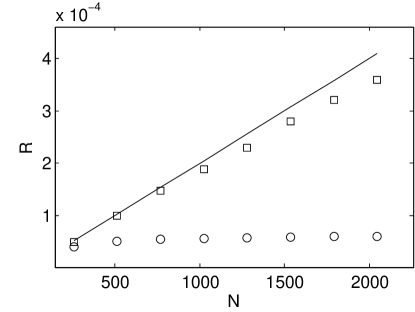
Figure 5: Fixation rate, $R$, versus system size for the 1D model (circles) and the well-mixed model (squares) with $U=10^{-5}$. $v$ quickly saturates in 1D but diverges for the well-mixed model. Solid line is the non-interfering fixation rate (4).

III Similarity to Surface Growth

It is illustrative to exploit the similarity between our model and surface growth. In surface growth phenomena, the width or standard deviation of the interface grows initially in time as $\sigma\sim t^{\beta}$, where $\beta$ is the growth exponent, then reaches a steady state when the correlation length reaches the size of the system (Barabási and Stanley, 1995; Family and Vicsek, 1985). In the steady state $\sigma\sim N^{\alpha}$ where $\alpha$ is the saturation exponent. We found the width or standard deviation of the distribution of fitnesses also follows power-laws with critical exponents as a function of $N$ and $U$.

By averaging over many simulations we found the transient values of $\sigma$ in figure 6. The width increased as $\sigma\sim t^{\beta}$, although $\beta$ was slightly dependent on $U$. At high $U$, $\beta$ was close to one half.

Figure 6: Time evolution of the standard deviation of the fitnesses $\sigma$ with $N=512$, $s=0.01$ and $U=10^{-3}$ (circles), $U=10^{-4}$ (squares), and $U=10^{-5}$ (crosses). The dashed lines are $\sim t^{1/2}$ The width approaches a stationary value as a power law with time $\sigma\sim t^{\beta}$, where $\beta$ is the growth exponent. $\beta$ is approximately $1/2$ for high $U$, and increases slightly as $U$ gets smaller.

From the simulation we also found the scaling of the steady-state width. In the single-fixation regime we would expect $\sigma$ to be small since most of the time the system has uniform fitness. Figure 7 shows $\sigma$ in multiple-mutation regime to be a power law: $\sigma\sim U^{\eta}$ with $\eta=0.3-0.4$. The width is also shown to go as $\sigma\sim N^{\alpha}$ and $\alpha$ is close to $1/2$.

Our model has a growth exponent close to $1/2$, which differs from the linear Edwards-Wilkinson universality class ($\beta=1/4$) and the non-linear KPZ universality class ($\beta=1/3$) (Barabási and Stanley, 1995). However, we found that the growth of the width changes for larger system sizes and longer time scales, which will be described in future work.

Figure 7: Top: Stationary standard deviation $\lim_{t\to\infty}\sigma(t)$ versus mutation rate $U$ with $N=512$ and $s=0.01$ averaged over $10^{5}$ mutations. The dashed line is $\sim U^{1/3}$ Bottom: width increases with system size as a power law with a characteristic exponent, with $U=10^{-5}$. The dashed line is $\sim N^{0.45}$.

IV Discussion

The model we study is restricted to one organism per site, as in (Gordo and Campos, 2006), in contrast to more detailed models divide a population into islands or demes, each with a finite well-mixed population. However, the one organism per site model may be approximated as a deme model with some restrictions by grouping together sites into demes (Korolev et al., 2010). The number of organisms per site affects the speed of the genetic wave that sweeps each mutation to fixation. Since genetic stochasticity is strong when there is one organism per site, the speed of the genetic wave front is $v_{F}\sim s$, as in (Doering et al., 2003),(Hallatschek and Korolev, 2009). In the weak noise limit, when population in the demes are relatively large and genetic drift is small, the genetic wave front moves with the speed $v_{F}\sim\sqrt{s}$ (Fisher, 1937). Also, we have not included a measure of the spatial dispersal of organisms after reproduction. In any case, changing the genetic wave speed would change $t_{\textrm{fix}}$, and therefore change the transition at which interference occurs. Notably if $v_{F}\sim\sqrt{s}$, then $U_{\textrm{tr}}$ would depend on $s$. However, the fixation time dependence on the total system size would not change since each island must be visited sequentially regardless of wave speed. Therefore we expect our main result that $R$ saturates with large $N$ will not change. Similarly, generalizing $s$ to a distribution of beneficial effects, would affect the time-scale of fixation, but we still expect $R$ to saturate with large $N$. We confirmed this with an exponential distribution of $s$ (not shown).

We have shown that spatial structure significantly affects the rate of fixation in our model. In the multiple-mutation regime, the rate of fixation is reduced and becomes independent of $N$ for large $N$, similar to neutral fixations. Since beneficial mutations do not have an overwhelming advantage over neutral and deleterious mutations, it would be interesting to study a more general distribution of fitness effects. It is possible for harmful mutations alone to accumulate in one dimension when they are common enough (Hallatschek and Nelson, 2010).

One dimensional populations have been used to model the frontiers of expanding bacterial colonies, when the organisms at the frontier reproduce faster than those in the interior (Korolev et al., 2010), although there are complications with boundary instabilities and boundary growth. We hope that similar experiments could test our prediction that the rate of fixation is independent of $N$.

A 2D version of our model could be representative of waves of spreading mutations in an immobilized population. This would be interesting to study since differences from the well-mixed model have already been observed in simulation and experiment (Campos et al., 2008; Gordo and Campos, 2006; Perfeito et al., 2006, 2008; Rosas et al., 2005), and system size dependence has not been investigated.