Spin-glass behavior in Ni-doped La_1.85Sr_0.15CuO₄

Abstract

The dynamic and static magnetic properties of La_1.85Sr_0.15Cu_1-yNi_yO₄ with Ni concentration up to $y$=0.63 are reported. All the features that characterize the spin-glass (SG) behavior are found: bifurcation of the dc susceptibility $\chi$ vs temperature curve, a peak in the zero-field cooling branch of this curve accompanied by a step in the imaginary part of the ac susceptibility $\chi_{ac}$, frequency dependence of the peak position in the real part of $\chi_{ac}$ and scaling behavior. The decay of remnant magnetization is described by a stretched-exponential function. The characteristic time from the critical slowing-down formula that governs the dynamics of the system suggests the existence of the spin clusters. The strongest interactions between the fluctuating entities are at $y$ equal to the charge carriers concentration in the system. The SG transition temperature decreases linearly with decreasing $y$ for $y$$\leq$0.30 and extrapolates to 0 K at $y$=0 what means that Ni display a magnetic character in the surrounding Cu-O network starting from the smallest concentration $y$. The static critical exponents characterizing the scaling behavior of the nonlinear part of $\chi$ lie between those typical for three dimensional Ising-like and Heisenberg-like systems.

I Introduction

Transition-metal oxides (TMO) seem to be a nature’s playground where a strong interplay between spin, charge, and lattice degrees of freedom appears. When doped with holes, their phase diagram involves spin- and charge-density-waves, Jahn-Teller distortions, ferroelectricity and superconductivity, to mention only few of their complex ground states.Bishop (2004) The spin-glass (SG) phase is also quite common to the phase diagram of TMO and has been observed, among others, in cobaltites,Wu and Leighton (2003); Phan et al. (2004) manganites,Salamon and Jaime (2001); Laiho et al. (2001) nickelates Lander et al. (1991); Freeman et al. (2006) and cuprates.Chou et al. (1995); Niedermayer et al. (1998) This can be viewed as a natural consequence of a disorder present in such complex systems due to their chemical doping with heterovalent cations.Dagotto (2005); Hasselmann et al. (2004); Alloul et al. (2009)

In the phase diagram of cuprates, the region displaying the SG features separates the antiferromagnetic (AF) and superconducting (SC) regions and its characteristics are observed even inside the SC dome.Niedermayer et al. (1998); Julien (2003); Mitrović et al. (2008) Glassines of spins, accompanied by charge glass-like behavior, seems to emerge with the first added holes.Panagopoulos and Dobrosavljević (2005); Raičević et al. (2008) At low temperatures, these holes localize, presumably at oxygen sites, and form a local singlet on the Cu sites.Zhang and Rice (1988) The magnetic frustration may be understood as a result of local ferromagnetic exchange coupling between Cu²⁺ ions in the background of three-dimensional (3D) long-range AF order.Aharony et al. (1988) The specific role of holes, including their self-organization in the stripes, and the details of the AF order, including the possible existence of the spin spirals, are still under debate.Kivelson et al. (2003); Hasselmann et al. (2004); Lüscher et al. (2006) The early observations of the spin dynamics and its evolution with doping have indicated that the entities undergoing the SG transition are the finite-size AF domains, cooperatively freezing in the inhomogeneous but magnetically ordered phase. Cho et al. (1992); Niedermayer et al. (1998) Thus this phase is often refereed to as a cluster SG. While the thermodynamical SG-type behavior here is well established, the microscopic origin is still discussed.Chou et al. (1995); Sanna et al. (2010)

The essential nature of cuprates is believed to be governed by the physics of the Cu-O planes, which are sometimes regarded as ideal 2D Heisenberg spin systems. However, any practical realization of such idealized layers is connected with introducing some inevitable, internal, disorder.Alloul et al. (2009); Coneri et al. (2010) Although the sources of such a disorder can be cuprate-family specific (such as, for example, the tilted CuO₆ octaedra and the stripe structure around $x$=0.12 in La_2-xBa_xCuO₄), the random distribution of Coulomb impurity potentials in the layers separating the Cu-O planes is the most common origin. Introduction of heterovalent dopants or extra oxygen atoms is necessary to change and control the charge-carriers concentration in cuprates but creates a modification of the Coulomb potential that disrupts the lattice periodicity and thus serves as an additional scattering center for carriers in the Cu-O planes.Alloul et al. (2009)

It is natural that the above-mentioned internal Coulomb-driven disorder is minimal in these compounds in which the carrier reservoirs are located far from the Cu-O layers. For example, the compounds such as HgBa₂CuO₄ and YBa₂Cu₃O_6+y (YBCO) are close to the cuprate clean limit.Dagotto (2005); Yang et al. (2009); Coneri et al. (2010) Doping with Ca allows to move the YBCO apart from the clean limit in a controlled way. The recent muon-spin-rotation ($\mu$SR) experiments on this system give the arguments against the picture of the cluster SG phase introduced by disorder and suggest the common ground state, named frozen antiferromagnet(FAF), both for low-doping regime (i.e. in the re-entrant AF phase) and for larger dopings for which clusters of spins coexist with percolating superconductivity.Sanna et al. (2010); Coneri et al. (2010) The study shows that the local-field distribution is narrow, in the strong contrast to the canonical SG in which the distribution width is comparable to the mean value. The disorder does not modify significantly the hole-concentration dependence of the FAF transition temperature. The origin of FAF remains unknown but dilution of magnetic moments, not frustration, seems to play the crucial role.Coneri et al. (2010)

The situation in the dirty cuprates, such as La_2-xSr_xCuO₄ (LSCO), is even more complicated because of the intrinsic disorder. In LSCO, in contrast to the clean-limit compounds, the cluster SG ”order” governs solely the physics of the system in a quite large region of the phase diagram. The hole-doping dependence of irreversibility in magnetization, which is found in LSCO, has been interpreted in terms of a generic quantum glass transition,Panagopoulos et al. (2002, 2004); Panagopoulos and Dobrosavljević (2005) it has also been suggested to be linked to the presence of the SC correlations above $T_{c}$,Freeman et al. (2006) and, recently, has been re-interpreted as an argument towards existence of spin-density-wave quantum critical point.Sachdev (2010) The NMR measurements have revealed the enhancement of spin-freezing temperature, $T_{g}$, deeply in the SC phase of LSCO at $x$$\simeq$0.12 and insensitiveness of this phenomenon to 1% of atomic disorder.Mitrović et al. (2008) Whether the physics underlying the cluster SG phase in the nonsuperconducting region of LSCO phase diagram and that at $x$$\simeq$0.12 is the same, is an open problem. The observation of charge glass-like behavior in lightly doped LSCO rises a question of how this dynamic charge order evolves into SC state with increasing $x$.Raičević et al. (2008) Clearly, the interplay between superconductivity and magnetic and electronic glassiness in LSCO is far from being well understood.

Impurities intentionally introduced into the Cu-O planes have been widely employed to probe the properties of cuprates, with the hope that the response of the system reveals the generic features of the pure compound. So far, such a situation close to being perfect has been found only in the 1D correlated systems. The magnitude of magnetization induced in quasi-1D AF spin chain Y₂BaNiO₅ by different nonmagnetic impurities appeared to decay exponentially, with the correlation length $\xi_{imp}$ equal to the numerical prediction for the spin-spin $\xi$ in the pure system.Alloul et al. (2009) In quasi-2D cuprates, the spinless defects in the Cu-O planes induce paramagnetic moments on the surroundings Cu ions and disorder driven by this local magnetism extents the SG region in the phase diagram in comparison to the pure system. As a result, the phase diagram of Zn-doped clean-limit YBCO becomes similar to that of non-doped dirty-limit LSCO.Mendels et al. (1994) This may be viewed as an argument that intrinsic or extrinsic - magnetically driven in this case - disorder influence the system in the similar way.Alloul et al. (2009)

In the context of the above, Ni is an unique dopant in cuprates. This results from its ability to built NiO₆ octaedra - increasing the substitution of Ni ions into the Cu-sites in LSCO leads eventually to isostructural nickelate La_2-xSr_xNiO₄ (LSNO). Although superconductivity is not observed in LSNO, its phase diagram is still very reach. The static 1D charge ordering in the form of stripes, predicted in the context of high-T_C superconductors (HTSC) Zaanen and Gunnarsson (1989); Machida (1989); Schultz (1989) has been first observed in LSNOHayden et al. (1992) and only later in Nd-doped LSCO.Tranquada et al. (1995) The proximity of the charge ordering region to the SG phase suggests that they may be related.Freeman et al. (2004, 2006) Thus, a systematic examination of the evolution of the LSCO properties with the Ni doping may shed some light onto the problem of possible correlation between superconductivity, stripe order and the SG phase in HTSC.

A remarkable evolution of views on the role of Ni dopant in cuprates has taken place, owing to accumulation of new experimental facts. Although nominally magnetic (3d⁸, S=1), Ni²⁺ ion appears to have weaker effect on superconductivity than the nominally non-magnetic Zn²⁺ (3d¹⁰, S=0) ion.Pines (1997); Mendels et al. (1999); Kofu et al. (2005) The dc susceptibility, $\chi$, measurements have revealed very small (0.6 $\mu_{B}$) paramagnetic moment of Ni introduced into the Cu-O planes.Xiao et al. (1990) It has been suggested that at small concentration Ni is substituted as Ni³⁺ ion.Nakano et al. (1998) The normal-state electrical transport experiments have suggested that the quasiparticle scattering at the Ni impurity has predominantly non-magnetic character.Hudson et al. (2001) On the other hand, the $c$-axis optical conductivity measurements in underdoped NdBa₂Cu₃O_6.8 show strong enhancement of the normal-state pseudogap energy by the Ni doping while doping with Zn is found to suppress the pseudogap. This different impact on pseudogap has been attributed to the magnetic character of the Ni dopant.Pimenov et al. (2005)

Just recently, it has been claimed that the Ni does not disturb the AF spin-1/2 network in the Cu-O planes when its concentration, $y$, is smaller than the hole concentration, $p$, in the system.Hiraka et al. (2009) The careful measurements of the local distortions around the Ni ions replacing Cu ions in La_2-xSr_xCu_1-yNi_yO₄ suggest that for small concentrations, $y\leq p$ (where $p$ is equal to Sr content, $x$), Ni serves only as a hole-absorber and creates a strongly hole-bond state, called Zhang-Rice doublet,Zhang and Rice (1988) with the effective moment S=1/2 that couples AF with S=1/2 moments of the surrounding Cu ions. These measurements have been carried out on the single crystals in a wide $p$-range ($p$=$x$, 0$\leq$x$\leq$0.15) but within limited Ni concentration ($y$$\leq$0.07). Based on them, a magnetic-impurity picture for Ni dopant in superconducting cuprates has been completely disqualified, at least below the optimally doped regions.Hiraka et al. (2009)

Our study shows that the actual situation is much more complicated. We have carried out the dynamic and static magnetic measurements of polycrystalline samples of La_1.85Sr_0.15CuO₄ (LSCO15) doped with Ni up to large concentration $y$=0.63, exceeding $p$ (equal to $x$=0.15 holes per CuO₂ plane) over four times. We have found the SG behavior in all non-superconducting samples, even in these with small $y$, below $p$. The transition temperature $T_{g}$, when extrapolated inside the SC region, takes finite values and approaches zero in the $y$=0 limit. Thus, the magnetic role of Ni should not be neglected even for $y<p$. Despite the microscopic mechanism, the low-temperature phase of Ni-doped LSCO exhibits all features characteristic for the SG systems: irreversibility in the $T$-dependence of $\chi$, a peak in the zero-field cooling (ZFC) branch of the $\chi(T)$ curve accompanied by a step in the imaginary part of ac-susceptibility $\chi_{ac}$, the moderate (typical for the cluster SG) frequency dependence of the peak position in the real part of $\chi_{ac}$, and the scaling behavior.

II Experimental details

The policrystalline samples of La_1.85Sr_0.15Cu_1-yNi_yO₄ (LSCNO) with 0$\leq$y$\leq$0.63 were synthesized from 4N-5N pure La₂O₃, SrCO₃, CuO and NiO by using conventional solid-state reaction method. The stoichiometric amounts of the powders were carefully mixed, pressed into pellets and sintered in a pure oxygen gas flow at 1320 K for 48 hours. After cooling down to room temperature with the rate 2 K/min, the samples were reground and the whole procedure was repeated two times.

The X-ray diffraction measurements were carried out at the Bragg-Brentano diffractometer (X Pert Pro Alpha1 MPD, Panalytical, with a setting described in Ref. [Paszkowicz, 2005]). For determination of absolute value of unit cell parameters, NIST SRM 676 Alumina was used as an internal reference material. Crystallographic characterization and structure refinement was done with help of FullProf.2k program.Rodriguez-Carvajal (2001)

The magnetic susceptibility measurements were carried out at two setups: the commercial SQUID magnetometer (MPMS, Quantum Design) working in the temperature range 2 K - 400 K and field up to 5 T (dc and ac measurements) and the home-build setup based on Cryogenics Consultants SQUID sensor and working in the temperature 1.6 K - 280 K and magnetic field up to 0.3 T (a part of the dc measurements).

III Results

III.1 Crystallographic analysis

Structural and phase analysis has shown that all samples have tetragonal K₂NiF₄-type structure (space group I4/mmm) and include no impurity phases. An example of Rietveld refinement plot is shown in Fig. 1 for LSCNO with the Ni content y=0.19.

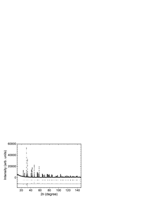
Figure 1: The x-ray powder-diffraction pattern of La_1.85Sr_0.15Cu_0.81Ni_0.19O₄. The observed pattern is denoted by dots while the calculated one is marked as solid line overlaying them. The bottom curve shows the difference between them. The short vertical lines mark the positions of Bragg reflections.

The lattice parameters of the undoped La_1.85Sr_0.15CuO₄ sample are a=3.77709(8) Å and c=13.2368(4) Å; thus, the axial ratio c/a is equal to 3.5045(2). The powder diffraction patterns indicate absence of any structural phase transition in the whole investigated range of the Ni content. The lattice constants change linearly with increasing $y$: $c$ decreases with the rate d$c/\text{d}y=-5.9(1)\times 10^{-3}$ Å ($\approx$0.02% $c$) per 1 at.% of Ni while $a$ increases with the rate d$a/\text{d}y=8.1(1)\times 10^{-4}$ Å ($\approx$0.05% $a$) per 1 at.% of Ni (see Fig. 2). As a result, the $c/a$ ratio decreases with the rate about 0.07% per 1 at.% of Ni. These results are consistent with the results of the earlier studies for a large Ni-doping range,Wu et al. (1996); Zhiqiang et al. (1998) but show a considerably smaller scatter of the experimental points. The d$c/\text{d}y$ and d$a/\text{d}y$ rates found here for $y\leq 0.63$ are comparable to the rates found for $y\leq 0.06$ in the detailed X-ray-absorption fine-structure (XAFS) and X-ray powder diffraction (XPD) measurements reported in Ref. [Haskel et al., 2001].

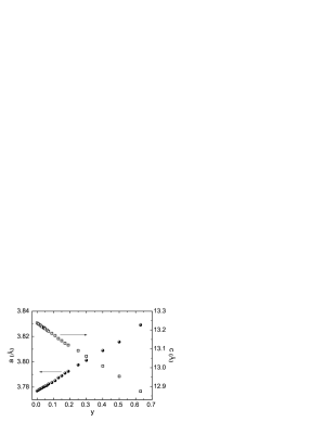
Figure 2: Lattice constants of LSCNO at room temperature as a function of Ni doping.

Free coordinates of the atoms in the tetragonal unit cell of LSCNO have been determined with the use of the Rietveld refinement procedure. Position (0,0,z) of the apical oxygen atom O(2) as a function of Ni content is discussed in Appendix A. Unlike the XAFS technique, XPD is not atom-specific in the sense that only averaged interatomic Cu/Ni-O(2) distance can be obtained. However, the detailed analysis (see Appendix A) suggests that Ni-O(2) distance may change between $y$=0.07 and $y$=1.

The bond length between the Ni atom and the in-plane oxygen atom O(1), Ni-O(1), has been found by XAFS measurements to have two distinct values, depending on the ratio of the hole concentration to the Ni content.Hiraka et al. (2009) As mentioned, the XPD technique is not capable of revealing such atom-specific details. Since the O(1) position, ($\frac{1}{2}$,0,0), is constant in K₂NiF₄-like structure of LSCNO, the averaged value of Cu/Ni-O(1) distance, resulting from the XPD analysis, increases with $y$ in proportion to lattice parameter $a$, i.e. with the same rate $\Delta a/(a\Delta y)$. This means contraction of Cu(Ni)O₆ octahedra along the $c$ axis with increasing Ni content, accompanying by simultaneous expansion in the $ab$ plane. The resulting volume change in the whole doping range is very small, of the order of 0.1%. More details on analysis procedure, free atomic positions and bond distance will be given elsewhere.Min

III.2 Normal-state dc susceptibility

The measurements of $\chi(T)$ at 10 Oe reveal that the superconductivity survives in LSCNO up to y=0.054.

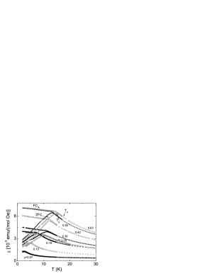
Figure 3: The low-temperature dc-susceptibility of LSCNO measured at 10 Oe for various Ni content, $y$. As an example, the ZFC and FC branches of $\chi(T)$ curve and the characteristic temperatures, $T_{g}$ and $T_{irr}$, are indicated for $y$=0.63 sample by arrows.

Above this Ni concentration, the normal-state $\chi$ vs $T$ curves display bifurcation below a characteristic temperature, $T_{irr}$, depending on the thermal-magnetic history of the sample, i.e. whether it was cooled down in the zero magnetic field (ZFC mode) or in the non-zero field (FC mode). The representative curves are shown in Fig. 3. The ZFC branch has a rounded but very well defined peak, position of which, $T_{g}$, is slightly below $T_{irr}$. Let us note that in the canonical SG usually an opposite situation is observed, i.e. $T_{irr}\lesssim T_{g}$. The behavior observed in LSCNO can be a manifestation of the existence of magnetic clusters in the system.Marcano et al. (2007)

The temperature of the peak in the ZFC $\chi(T)$ curve, $T_{g}$, which we take as the temperature of a transition to the SG phase, increases linearly with $y$ up to $y$=0.30 (see the inset to Fig. 4). The smallest concentration $y$, for which we observe the bifurcation of $\chi(T)$ curve, is equal to 0.056. The temperature $T_{g}$, when extrapolated linearly outside our temperature measurement window and inside the SC phase, has finite values and decreases to zero at $y$=0 (see the solid line in the inset to Fig. 4). This strongly suggests that Ni dopant in the sublattice of surrounding Cu spins displays a magnetic nature starting from the smallest concentration $y$.

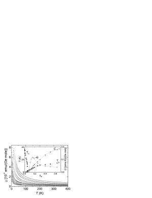
Figure 4: The dc-susceptibility of LSCNO, measured at 1 kOe field, for Ni content, $y$, equal to (from bottom up) 0.09, 0.11, 0.13, 0.15, 0.17, 0.19, 0.25, 0.30, 0.50 and 0.63. The solid lines are the best fits to the Curie-Weiss law in the 30 K - 400 K range. Inset shows the characteristic temperatures $T_{C}$ and $T_{g}$ and effective fitting parameter $\theta$ (left scale) as a function of $y$. The solid line is the linear fit to $T_{g}$ vs $y$ dependence for $y\leq 0.30$. In addition, the fitting parameter C is shown as a function of $y$ in the whole doping range (right scale). The dashed lines are guides to the eye.

It should be emphasized that the deviation of $\chi(T)$ measured in the FC mode from that measured in the ZFC mode cannot alone prove that a SG state develops below the bifurcation temperature of $\chi(T)$ curve. The superparamagnetic systems and conventional ferromagnets with a broad distribution of potential barriers exhibit such a feature as well. In addition, the ZFC-FC splitting of $\chi(T)$ is observed in disordered AF compounds that may be more relevant to the LSCNO system.K rner et al. (2000) Thus, in the next sections, we will present the additional characteristics confirming the transition to the SG phase: a logarithmic frequency dependence of the real part of ac susceptibility, $\chi^{\prime}$, below the transition, a step in the imaginary part, $\chi^{\prime\prime}$, a small frequency dependence of the peak position in $\chi^{\prime}(T)$ curve, described by the standard critical slowing-down formula, time decay of the thermoremnant magnetization and, finally and the most conclusive, the scaling behavior of the nonlinear dc-susceptibility.

Before that, however, we will shortly describe the $\chi$ behavior at temperatures well above $T_{g}$. The normal-state $\chi(T)$ at larger temperatures for Ni concentration below $y$=0.09 can be analyzed in terms of the universal empirical curve $F$, proposed for LSCO without parametrization independently by JohnstonJohnston (1989)and Nakano.Nakano et al. (1998) The universal function $F$ was found to describe the effective susceptibility of the Cu²⁺ spin sublattice in LSCO with various Sr content when the $\chi(T)$ data are represented in the reduced parameters $(\chi-\chi_{0})/(\chi-\chi_{max})$ and $T/T_{max}$, where $\chi_{0}$ is the $T$-independent sum of three components: (1) - the isotropic contribution from the closed Cu shells, (2) - the Van Vleck contribution and (3) - the contribution from the charge carriers, and $\chi_{max}$ is the maximal value that $\chi(T)$ reaches at $T_{max}$. Using the universal function from Ref. [Nakano et al., 1998], we have fitted $\chi(T)$ to the formula $\chi(T)=\chi_{0}+A\cdot F(T/T_{max})+C/T$ and have calculated the effective magnetic moment introduced by Ni ion, $\mu_{eff}$, from the Curie term, $C/T=N\mu^{2}_{eff}/3k_{B}T$, with the rest of parameters having their usual meaning (see Ref. [Malinowski et al., 2010]). The moment $\mu_{eff}$ is constant up to $y$=0.07 and equal to $(0.7\pm 0.05)\mu_{B}$ per Ni ion, what is very close to the value found previously when a linear function instead of $F$ has been used in the analysis.Xiao et al. (1990) Note that there is no need to add any finite paramagnetic Curie temperature, $\theta$, in the Curie term to reproduce the experimental data well, as it was necessary for Ni-doped LSCO with x=0.18 Sr content.Ishikawa et al. (1992)

The $\chi(T)$ term described by the $F$ function is not detectable when Ni concentration exceeds $y$=0.09. For these large $y$, the $\chi(T)$ data above $\sim$30 K are well reproduced by the Curie-Weiss (CW) law, with the finite negative $\theta$, $\chi=\chi_{0}+C/(T-\theta)$. The best fits are shown by the solid lines in Fig. 4. The calculated magnetic moment $\mu_{eff}$ does not remain constant, as it does for smaller $y$, and increases with increasing $y$ to reach about 1.6 $\mu_{B}$ per the Ni ion for $y$=0.5. Assuming temporary that all Ni ions are in the same magnetic state this would mean that the spin of Ni ion is much closer to $S$=1/2 (for which $\mu_{eff}$=1.73 $\mu_{B}$) than to $S$=1 ($\mu_{eff}$=2.82$\mu_{B}$). Note that the identical value (1.6$\pm$0.1$)\mu_{B}$ was obtained for Ni-doped YBa₂Cu₃O_6+x, where Ni moment remains quasi-constant with hole doping in the investigated range up to $y$=0.04.Mendels et al. (1999)

The CW term in the temperature dependence of susceptibility indicates the presence of the localized magnetic moments in the system. For small $y$$<$$0.09$, when the magnetism of the Cu-ions sublattice is clearly described by the function $F$ and it is not much altered by the Ni ions introduced in small quantities, the Curie term in $\chi(T)$ can be fully attributed to Ni ions, all being in the same magnetic state.Xiao et al. (1990) The resulting $\mu_{eff}=g\sqrt{S(S+1)}=0.7\mu_{B}$ means that the spin $S$ of Ni ion, immersed in the surrounding Cu ions sublattice, is equal to 0.11. Such a small value can be explained by the formation of the strongly hole-bound state of Ni ion, represented as Ni²⁺L, as proposed in Ref. [Hiraka et al., 2009]. However, we observe the increase of the $\mu_{eff}$ starting at $y$$\approx$0.09, not at $y$=0.15 (being equal to the hole concentration in the system), as it is expected from the picture suggested in Ref. [Hiraka et al., 2009]. Abrupt increase of the $C$ in the CW law for $y$$>$0.07 suggests that at least part of the Ni ions is in the magnetic state different from Ni²⁺L, even at concentration below $y$=0.15. However, the macroscopic susceptibility measurements alone do not allow to separate out the observed effective moment into two components coming from the Ni ions in two different magnetic states.

The values of $\theta$ for a given $y$ display some dependence on the $T$-range used in fitting $\chi(T)$. This makes to treat $\theta$ as the effective parameter rather than the true constant. In addition, there might be some crystal electric field effects, averaged in the policrystalline samples. Nevertheless, the negative sign of the effective paramagnetic CW temperature $\theta$ indicates that the dominant exchange interactions in the system are antiferromagnetic. As it is shown in the inset to Fig. 4, the $\theta$ exhibits strong dependence on Ni content. Its absolute value, $|\theta|$, increases abruptly when $y$ increases from $y$$\approx$0.09 up to $y$=0.15 This is followed by a rapid decrease, and a regime of saturation for $y$$>$0.30 (with a weak tendency to decrease with increasing $y$). This behavior can be understood as a result of trapping the mobile holes by the Ni ions and will be discussed in the Sec. IV.3.

III.3 Ac susceptibility

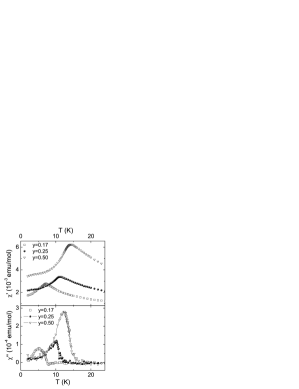
Figure 5: The real $\chi^{\prime}$ and imaginary $\chi^{\prime\prime}$ components of the ac susceptibility of LSCNO with y=0.17, 0.25 and 0.50 Ni content as a function of temperature, measured at f=1 Hz and with 1 Oe amplitude of the applied ac field and without any dc-bias.

The metastable SG state is usually characterized by ac susceptibility, $\chi_{ac}$. In Fig. 5 we show $\chi_{ac}(T)$ curves for LSCNO for several Ni contents, $y$=0.17 (LSCNO17), $y$=0.25 (LSCNO25) and $y$=0.50 (LSCNO50). A quite sharp cusp is visible in the in-phase component, $\chi^{\prime}(T)$, for all samples. Its temperature, $T_{f}$, is always a bit larger than the temperature of the maximum in dc-$\chi(T)$, $T_{g}$, and roughly coincidences with the temperature of the inflection point in the step of the out-of-phase component, $\chi^{\prime\prime}(T)$. At larger temperatures, above $T_{f}$, $\chi^{\prime\prime}(T)$ is equal to zero, while below $T_{f}$ has a finite value. Such a behavior is characteristic for SG transition and allows to distinguish the SG compounds from the disordered AF systems, in which $\chi^{\prime\prime}(T)$ is constant and remains equal to zero even below the temperature of the transition.K rner et al. (2000); Süllow et al. (1997); Mulder et al. (1982)

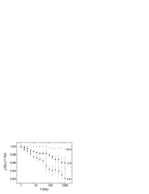
Figure 6: Normalized real part of $\chi_{ac}$ for LSCNO25 as a function of frequency for different temperatures - above and below $T_{g}$. The amplitude of ac field was 1 Oe and the measurements were carried out in 10 Oe dc field. The error bars for the frequency scan at $T$=25 K are similar to these for the scans at 2 K and 8 K.

In Fig.6 we depict the real part of $\chi_{ac}$, normalized to the value at 1 Hz, as a function of frequency for LSCNO25, as an example. At 25 K, i.e. above $T_{g}$, in the paramagnetic state, the variation of $f$ over three decades does not influence $\chi^{\prime}$ in a noticeable way. Below $T_{g}$, in the SG state, the $\chi^{\prime}$ exhibits a logarithmic frequency dependence. Such a frequency dependence has been predicted theoretically for a short-range Ising SGFisher and Huse (1986) and it has been observed for many SG systems.Giot et al. (2008) However, this logarithmic relationship is not unique for the SG, because it is exhibited by any two-level disordered system, dynamics of which is governed by activated processes with a broad distribution of the activation barriers heights.Pytte and Imry (1987) Note that at 8 K, closer to $T_{g}$, the system is more sensitive to variation of frequency then at 2 K, ”deeper” in the frozen state.

The ac measurements at various frequencies reveal that the position of the maximum in $\chi^{\prime}(T)$ curve, $T_{f}$, moves toward higher temperature and the magnitude of $\chi^{\prime}$ decreases with increasing frequency. Such a behavior is expected for a SG system. As a raw measure of this frequency dependence, the parameter $\delta=d\text{ln}T_{f}(\omega)/d\omega$ is used.Binder and Young (1986) In experimental practice, a shift between two outermost frequencies accessible in experiment is usually employed and $\delta$ is calculated as $\delta=\Delta T_{f}/(T_{f}\Delta\text{ln}\omega)$.Mulder et al. (1982); Marcano et al. (2007) The values of $\delta$ obtained in this way for LSCNO system do not show any obvious correlation with $y$ and are equal to 0.012, 0.012 and 0.014 for $y$=0.17, 0.25 and 0.50, respectively.

For systems with noninteracting entities (which can be either particles or magnetic clusters), the values of $\delta$ of the order of 0.1 have been reportedJ. L. Dormann and Fiorani (1988) and such a relatively high sensitivity to frequency is predicted in the classical model of superparamagnetism.Néel (1949); Brown (1963) Any interactions between particles weakens this high sensitivity and this is why almost two orders of magnitude smaller values of $\delta$ are measured in the canonical spin glasses (e.g. $\delta$$\approx$0.002 for CuMn, Ref.[Mulder et al., 1981]) or in the SG phase of other systems, such as manganites, where $\delta$$\approx$0.003 is reported.Giot et al. (2008) Finally, in the case of well-ordered ferromagnetic or AF systems with even stronger interactions only MHz and GHz frequencies are sufficiently large to cause any observable shift in the $\chi^{\prime}(T)$ peak position.Mydosh (1993)

The values of $\delta\sim 0.01$ obtained for LSCNO lay between these extremes and are typical for cluster glasses, i.e. systems with randomly distributed interacting magnetic clusters.Li et al. (2005) Recently, $\delta=0.016$ was observed in Ce₂CuGe₃, which is an example of so called nonmagnetic atom-disorder SG system with possible (ferromagnetic) clusters.Tien et al. (2000) To recapitulate, the use of the simple but model-independent criterion based on the parameter $\delta$ strongly suggests the possibility of the existence of spin clusters in LSCNO. The frequency dependence of $T_{f}$ will be discussed in more detail in Sec. IV.2

III.4 Magnetic hysteresis

The presence of spin clusters should be reflected in the magnetic hysteresis. Evolution of the magnetization loops in LSCNO50 is illustrated in Fig.7, where the isothermal $M(H)$ curves are depicted at several temperatures.

Figure 7: Evolution of the $M$ vs $H$ behavior with temperature for y=0.50 sample. The $M-H$ isothermal curves are shown for 2 K (well below $T_{g}$=13.1K), 10 K (still below $T_{g}$), 17 K (between $T_{g}$ and $T_{irr}$) and 50 K (well above $T_{f}$). Insets show details at low fields at T=10 K and at T=17 K.

The curves for LSCNO17 and LSCNO25 have qualitatively similar features. No trace of saturation is visible even at the lowest $T$. At 2 K, the individual branches of the $M(H)$ curve obtained after ZFC have a characteristic ”S” shape - the initial slope of the curve is smaller than the slope at inflection point at nonzero field. This is particularly clearly visible in the virgin curve. Such ”S” shape of $M$ vs $H$ curve is typical for SG systems in a frozen state.Binder and Young (1986) With increasing temperature the S-shaped curve smoothly evolves into a straight line, indicating the paramagnetic behavior at high $T$. Hysteresis is observed only below $T_{g}$. The coercive field, taken from the hysteresis loops measured at 2 K, increases linearly with $y$ and is equal to 1.0, 1.4 and 2.6 kOe for y=0.17, 0.25 and 0.50, respectively. A high-field part of the virgin curve (above 9 kOe for y=0.50 at 2 K) lies outside the hysteresis loop. This suggests the presence of metastable states in the system.

The existence of a hysteresis loop clearly excludes superparamagnetism as a candidate for the ground magnetic state of LSCNO, since superparamagnetism is a thermal equilibrium behavior.Bean and Livingston (1959) In the case of ferromagnetic or canted AF clusters existing in the system, a hysteresis is expected but with large initial susceptibility because clusters are at first saturated along their local easy axis and only after that various clusters became fully aligned along the applied field.Marcano et al. (2007) If clusters reverse their magnetization coherently then hysteresis loops have almost rectangular shapes.Westerholt et al. (1986) In LSCNO just the opposite behavior is observed - the initial $\chi$ is smaller then this at inflection point in $M(H)$ curve. Thus, it is reasonable to conclude that $M(H)$ curves do not show any feature indicative of (large) clusters in LSCNO. The $M(H)$ curves remain non-linear for $T_{g}<T<T_{irr}$ indicating that SG phase starts to built over a broad T-range. For LSCNO25, nonlinearity in the $M$ vs $H$ dependence is observed even at 25 K, i.e. at $T\simeq 2.5T_{g}$, well above $T_{irr}$. The deviations of the $M(T)$ curve measured at constant field from the CW dependence fitted in a wide $T$-range (up to 400 K), appear at around 30 K. These features indicate that short-range AF correlations and fluctuations exist well above $T_{g}$. Such precursors of cooperative freezing at $T_{g}$ have been observed in metallic SG with $\theta$$>$0 at temperatures higher than 5$T_{g}$Morgownik and Mydosh (1981) and in the amorphous SG with both signs of $\theta$ at even higher temperatures $T$$\approx$$12-20T_{g}$.Morgownik and Mydosh (1982); Morgownik et al. (1984); Rao et al. (1983)

III.5 Decay of thermoremnant magnetization

Since the SG system in a frozen state can react to the applied field slowly, the magnetization curves obtained after ZFC procedure do not give information about the thermal equilibrium of SG but rather reflect a slow increase of magnetization (and thus susceptibility) with time.Binder and Young (1986) The underlying physics is similar to the one that governs the decay of the remanent magnetization with time.

To investigate the mechanism by which the system decays back to equilibrium we have applied a following procedure. First, the magnetic field of 1000 Oe has been turned on at 200 K. Subsequently, the sample has been cooled down to 200 K during 80 min, then the temperature has been kept constant for 10 min, and, finally, the magnetic field has been switched off. Next, the remnant magnetization has been measured vs time at $T=2$ K, starting immediately after the field became zero.

Figure 8: Time dependence of the thermoremanent magnetization $M_{TRM}$ for the LSCNO sample with y=0.25. $M_{TRM}$ is normalized to the value measured immediately after the field is set to zero, $M_{TRM}(0)$. The thick solid line is the best fits to a stretched exponential dependence, the dotted thin line - to Eq. (2) and the dashed one - to Eq. (3).

As it can be seen in Fig.8, the time decay of this FC thermoremanent magnetization, $M_{\text{TRM}}$, is well described by a stretched exponential formula,

$$M_{TRM}(t)=M_{0}\text{exp}[-(t/\tau)^{1-n}].$$ (1)

This form is commonly used to describe different relaxation phenomena, including magnetic, optical and mechanical ones, in different complex random systems with a distribution of relaxation times.V. Degiorgio and T.Bellini (1990); Str However, no generally accepted microscopic explanation of this behavior exists so far. Percolation model puts the restrictions on the possible values of stretching exponents, $1/3\leq 1-n\leq 1$.Lois et al. (2009) The values of $1-n$ below the mean-field value, 1/3, were reported, albeit they are believed to be non-intrinsicPhillips (1996) or related to fragility of some glass formers.Böhmer et al. (1993) The theory predicts that presence of the long-range forces (in addition to the obvious short-range forces) modifies the glassy relaxation dynamics, reducing $1-n$ (within the limits given above).Phillips (2006); Jund et al. (2001) The relationship (1) was theoretically predicted also for the SG systems.Continentino and Malozemoff (1986); Ogielski (1985); C. De Dominicis and Lainee (1985) The numerous experimental data on the canonical SG, such as, for example, Ag:Mn,Hoogerbeets et al. (1985) confirm validity of this formula for the description of the relaxation of magnetization in these systems.Binder and Young (1986) The best fit to Eq. (1) for LSCNO25 is visible in Fig. 8 as the solid line.

We have also tried to fit the data to other formulas used to describe decay of magnetization, a power law and a logarithmical dependence,

$$M_{\text{TRM}}(t)=M_{0}t^{-\gamma},$$ (2)

$$M_{\text{TRM}}(t)=M_{0}-S\text{ln}(t),$$ (3)

respectively.G. Sinha and Majumdar (1996) Eq. (2) has been used to describe relaxation of magnetization in the systems with both long-range-AF and long-range-ferromagnetic order.G. Sinha and Majumdar (1996); Patel et al. (2002) Numeric simulations predict that this equation should be also applicable to the SG systems.Kinzel (1979) Eq. (3) has been found to be valid for the systems where the energy barriers over which magnetic relaxation takes place are uniformly distributed from zero to a certain maximal energy and the behavior consistent with this equation has been observed in several different SG systems. Guy (1977, 1978); Dhar et al. (2003) It has been noted that when the decay parameter $\gamma$ is small, the experimental data in the limited time interval can be fitted both by Eq. (2) and Eq. (3) equally well.Kinzel (1979); Smith et al. (1994) In all these equations (1-3) $M_{0}$ is one of the fitting parameters but, as pointed out in Ref.[Tiwari and Rajeev, 2005], in Eq. (2) and Eq. (3) it depends on the time unit used (since this is a fitted value of $M_{TMR}$ at $t$=1). The dotted line presented in Fig.8 is the best fit to Eq. (2), while the dashed one is the best fit to Eq. (3). The magnetization is normalized by $M_{TRM}(0)$, the measured value of $M_{TRM}$ immediately after the field is set to zero. The measurement was sufficiently long ($\sim 8$ hours) to distinguish between the different possible functional forms, given by Eqs. (1)-(3). The quality of the best fits to the functions (2)-(3) is not satisfactory, as it can be easily seen in Fig. 8.

The calculated values of $\chi^{2}$ and correlation coefficient $R^{2}$ in the standard analysis unambiguously show that the stretched exponential form (1) is the best description of magnetization decay in LSCNO. The best fit to Eq. (1) gives $1-n=0.32\pm 0.01$. The parameter $n$ is in perfect agreement with theoretical predictions for the SG systems,Campbell (1986, 1988) with the simulations on a 3D Ising SGOgielski (1985) and with the experimental results on the canonical SG, which also give $1-n\approx 1/3$.Chamberlin et al. (1984)

IV Discussion

IV.1 Static scaling

The definitive feature that corroborates the presence of the SG phase in LSCNO is the scaling behavior. Introducing the SG susceptibility, $\chi_{SG}$, proportional to averaged (thermally and spatially)Fischer (1975); Sherrington and Kirkpatrick (1975) square of the spin correlation function, $\chi_{SG}\propto\displaystyle\sum_{i,j}[\langle S_{i}\cdot S_{j}\rangle^{2}_{T}]_{av}$, allows to analyze the SG transition within the framework of the second-order phase transition theory, with diverging correlations at $T_{g}$ and onset of the ”order” below $T_{g}$, and next to implement the static scaling hypothesisWidom (1965); Kadanoff (1966) to description of the SG.Fischer and Hertz (1991a)

Experimentally, the $\chi_{SG}$ is measurable through the dimensionless nonlinear susceptibility, defined as $\chi_{nl}(T,H)\equiv 1-M(T,H)/\chi_{l}H$.Chalupa (1977); Suzuki (1977); Omari et al. (1983) The linear susceptibility, $\chi_{l}$, comes from the measurements at low field. This definition of $\chi_{nl}$ means that the measured temperature-dependent susceptibility, $\chi\equiv M/H$, can be written as $\chi$=$\chi_{l}(1-\chi_{nl})$. Note that sometimes the term ”nonlinear susceptibility” refers in the literature to the coefficient at the third power of field in the expansion of magnetization in odd powers of field, $\partial^{3}M/\partial H^{3}|_{H=0}$. In the following, by $\chi_{nl}$ we mean the ”whole” nonlinear part of $\chi$.Dekker et al. (1988) To use $\chi_{nl}$ in the scaling analysis, one needs to stand up to the problem with estimation of the critical region where the scaling should hold and to the fact that the state below the SG transition temperature is not a state of thermodynamic equilibrium.Fischer and Hertz (1991b) Despite these difficulties, $\chi_{nl}$ has been found to be a good tool to investigate a possible thermodynamic phase transition in the various 2D and 3D SG systems.Beauvillain et al. (1984)

In Fig.9 we depicted the susceptibility of LSCNO25 measured at various fields from $\mu_{0}H$=10 Gs to 5 T.

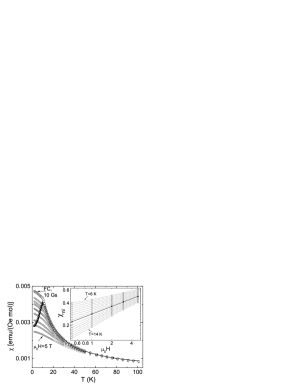
Figure 9: Magnetic susceptibility of LSCNO25 as a function of temperature at various fields. The large symbols denote ZFC (black spheres) and FC (open squares) data measured at $\mu_{0}H$=10 Gs. The solid line is the best fit of CW function (plus constant) to the FC data above 12 K. The small open symbols represent data measured at 0.02, 0.1, 0.2, 0.5, 1, 2, 3 and 5 T (from top to bottom) in the FC mode. In the inset, the open circles denote the nonlinear susceptibility $\chi_{nl}$ as a function of field at various temperatures at 0.5 K intervals, from 6 K to 10 K and from 11 K to 14 K (from top to bottom). The solid line is the best fit of the dependence (5) (see text) to the data at $T_{g}$=10.4 K (denoted as solid circles). The dashed lines are the guides to the eye.

The temperature-dependent part of the susceptibility at low field and at temperatures above $\approx$1.2 $T_{g}$ is well described by the CW dependence, $\chi(T)-\chi_{0}=C/(T-\theta)$. The best fit to the FC $\chi(T)$ data in the range 12 K - 100 K, showed in Fig.9 as the solid line, gives negative effective $\theta$=$-5.3\pm 0.1$ K, indicating the presence of the AF correlations. We will take only the $T$-dependent part of the measured $\chi$ into account in the following scaling analysis. We assume that $\chi(T)$ measured at 10 Oe is a good approximation of $\chi_{l}$ and thus $\chi_{l}=C/(T-\theta)$. At low temperatures, the magnetization increases nonlinearly with the field and the $\chi(T)$ deviates from the CW function towards the smaller values at larger fields, as it is clearly visible in Fig.9.

The scaling theory predicts for $\chi_{nl}$ the relationship

$$\frac{\chi_{nl}}{\mid t\mid^{\beta}}=f_{\mp}\left(\frac{H^{2}}{|t|^{\beta+\gamma}}\right),$$ (4)

where $t$ is the reduced temperature, $t$=$(T-T_{g})/T_{g}$, $\beta$ and $\gamma$ are the critical exponents, and $f_{-}$ ($f_{+}$) is the scaling function for $t<0$ ($t>0$).Suzuki (1977); Barbara et al. (1981); Malozemoff et al. (1983) (Another approach to the static scaling, sometimes used in the literature but clearly giving unsatisfactory results in the case of LSCNO, is discussed in Appendix B.) The scaling functions $f_{\mp}(x)$ behave as const$\cdot x^{2/\delta}$ in the large-$x$ limit.Chalupa (1977); Barbara et al. (1981) This means that right at $T_{g}$ we have

$$\chi_{nl}\propto(H^{2})^{1/\delta},$$ (5)

where $\delta$ is another critical exponent, related to $\beta$ and $\gamma$ by the scaling law

$$(\delta-1)\beta=\gamma.$$ (6)

In the inset to Fig.9 we present the $\chi_{nl}$ vs $H$ curves for various temperatures. They are results of the isothermal cross-cuts of the $\chi_{nl}(T)$ curves calculated from the experimental data for various fields. The position of the maximum in the ZFC $\chi(T)$ curve at 10 Oe, equal to 10.4$\pm$0.1 K, is taken as $T_{g}$. The $\chi_{nl}(H)$ curves on log-log scale change their curvature sign around $T_{g}$. Right at $T_{g}$, the data are described by a linear dependence on the log-log scale and the best fit to Eq. (5), shown in the inset as the solid line, yields $\delta$=5.8$\pm$0.1.

With this value of $\delta$ we have adjusted $\beta$ and have calculated $\gamma$ from Eq. (6) to obtain the optimum coincidence of the data on two universal curves, one for $t<0$ and second for $t>0$, in the $\chi_{nl}/|t|^{\beta}$ vs $H^{2}/|t|^{\beta+\gamma}$ plot. The best qualitative collapsing of the data to these two separate curves has been found for $\beta$=0.75, what implies $\gamma$=3.6 (see Fig.15 in Appendix B). We have estimated the uncertainty of the adjusted parameter to be $\sim$0.05, i.e. $\beta$=0.75$\pm$0.05 and thus $\gamma$=3.6$\pm$0.3.

To estimate and to visualize the critical temperature region where the scaling is valid, it is better to use the argument of the scaling function that is linear in $t$. Such improved form of the scaling has been proposed by Geschwind et al. for the equation $\chi_{nl}=H^{2\beta/(\beta+\gamma)}G(x)\equiv H^{2\beta/(\beta+\gamma)}G(H^{2}/|t|^{\beta+\gamma})$. Geschwind et al. (1990) Raising the argument $x$ to the power of $-1/(\beta+\gamma)$ makes it linear in $t$. In the same way, Eq. (4) may be reformulated as

$$\frac{\chi_{nl}}{\mid t\mid^{\beta}}=\tilde{f}_{\mp}\left(\frac{|t|}{H^{\frac{2}{\beta+\gamma}}}\right).$$ (7)

The scaling plot with the use of this equation for $\beta$=0.75 and $\gamma$=3.6 is presented in Fig. 10.

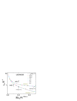
Figure 10: (Color online) Scaling plot for LSCNO25 according to Eq. (7) with $\beta$=0.75 and $\gamma$=3.6 for the nonlinear susceptibility $\chi_{nl}$ at various magnetic fields from 0.1 T to 5 T at temperatures below ($t$$<$0) and above ($t$$>$0) the SG-transition temperature $T_{g}$=10.2 K. The error bars are of the symbol size.

In the logarithmic scale of $y$-axis all values of $\chi_{nl}|t|^{-\beta}$, varying over two decades, are given equal weight and this allows to notice and compare any potential deviations from the universal curves at different ordinates. The scaling validity region at lower fields is noticeably smaller than at larger fields, i.e. the scaling does not work for the same argument $|t|/H^{2/(\beta+\gamma)}$ of function $\tilde{f}_{\mp}$ for which the scaling at larger fields is still valid. In terms of temperature critical region, this means that at the field 0.2 T scaling is valid in the interval $\sim 0.8T_{g}-1.1T_{g}$. The deviations of the data outside this $T$-region from the universal curves are larger than the measurements uncertainties (which are of the symbol size in Fig. 10). The scaling region expands with increasing field and the quality of scaling at 5 T is still excellent even at temperatures as far from $T_{g}$ as $0.2T_{g}$ (i.e. the lower limit of our measurement window) and $2T_{g}$. Such a large scaling region has been found experimentally to be typical for the canonical SG systems,Barbara et al. (1981) in agreement with the numerical simulations for the 3D Ising SG, by which the critical region has been estimated to extend up to $|t|\approx 0.55$.Ogielski (1985)

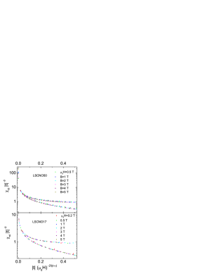
Figure 11: (Color online) Scaling plot for the nonlinear susceptibility $\chi_{nl}$ of LSCNO17 (LSCNO50) according to Eq. (7) with $\beta$=0.55 ($\beta$=0.75) and $\gamma$=3.2 ($\gamma$=3.8).

Results of the identical scaling procedure for LSCNO17 and LSCNO50 are similar to those for LSCNO25. In particular, the scaling according to Eq. (4) and its improved form, Eq. (7), gives clearly the better results than the scaling according to  Eq. (15). This remains true even for LSCNO17 where the strongest AF correlations among the investigated samples are expected and thus one might expect that the scaling approach described in Appendix B would work better than that described by Eq. (7). The best collapsing of the data at different magnetic fields onto two branches of the universal curve - below and above $T_{g}$ - have been found for LSCNO17 for $\beta$=0.55, i.e. the value closer to $\beta$=0.5, predicted by the numerical simulations for 3D Ising SG, than to $\beta$=1, predicted by the mean-field theory for isotropic 3D Heisenberg SG. The quality of scaling is excellent, as it can be seen in the bottom panel of Fig. 11. The scaling for LSCNO50 is best for $\beta$=0.75, i.e. for the same value as for LSCNO25. A comparable size of the $T$-region where the scaling is valid starts for LSCNO50 at larger fields than for LSCNO17 and LSCNO25, but the quality of the scaling is still very good (see the upper panel in Fig. 11).

The parameter $\beta$, found here as a result of simple adjusting procedure, is a critical exponent for the SG order parameter $q_{EA}$, originally introduced by Edwards and Anderson in the model based on the classical (mean-field) calculations.Edwards and Anderson (1975) The corresponding quantum-mechanical calculations have been carried out by Fischer.Fischer (1975) Since no lattice effects have been taken into account, the obtained results describe the amorphous SG, where the CW law with $\theta$=0 is found above $T_{SG}$.Fischer (1975) The possibility that the average exchange interaction $J$ is not zero, and thus causes that the ferromagnetic order competes with the SG phase, has been included into the model by Sherrington, Southern and Kirkpatrick (SSK), and the formula for extracting $q_{EA}$ from the measured $\chi$ has been given.Sherrington and Southern (1975); Sherrington and Kirkpatrick (1975); Kirkpatrick and Sherrington (1978) The calculations based on the local-mean-field approximation suggest that $q$ remains unchanged when $J$ changes its sign.Patterson et al. (1978) The one-component SSK model has been modified and extended subsequently to describe a two-component Ising-like magnetic system (with the separate order parameter for each component), where the re-entrant transition to the SG phase, both from the ferromagnetic and from the AF phase, is predicted.Korenblit and Shender (1985); Takayama (1988); Fyodorov et al. (1987) None of these models provides a realistic description of LSCNO. Due to lack of analytical expression for $q_{EA}$, the adjusting procedure seems to be the best approach to find $\beta$.

IV.2 Dynamical scaling

A more detailed insight into the dynamics of the SG state in LSCNO can be obtained from the analysis of the $\chi_{ac}$ measurements. In Fig.12 we depicted the temperature dependence of the real component of $\chi_{ac}$ for LSCNO25, measured with 1 Oe ac field amplitude at various frequencies.

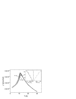
Figure 12: The real part of $\chi_{ac}$ as a function of temperature in the vicinity of the transition to the SG phase at various frequencies (from top to bottom: 1.00, 2.68, 7.19, 31.3, 138.7 and 997.3 Hz) for LSCNO25. The bottom inset shows the peak positions for this sample (open circles) together with those for LSCNO17 (solid squares) and LSCNO50 (solid diamonds). The thick solid lines are the best fits to Eq. 8. The details are described in the text and the obtained parameters are given in Table 1. In the upper inset, the slowing-down formula (Eq. 8) versus Vogel-Fulcher law (Eq. 9) is tested for description of experimental data for LSCNO25. The thick (thin) solid line in left (right) panel is the best fit to Eq. 8 (Eq. 9), correspondingly. Note the logarithmic scale of abscissa in the left panel and the linear one in the right panel.

The data have been collected after cooling the sample in zero field. The peak position $T_{f}$ moves toward higher temperature with increasing frequency. This frequency dependence can be described by the standard critical slowing down formula, given by the dynamic scaling theory,Hohenberg and Halperin (1977)

$$\tau=\tau_{0}\left(\frac{T_{f}-T_{g}}{T_{g}}\right)^{-z\nu}.$$ (8)

In this equation, the characteristic time $\tau$ describes the dynamical fluctuation time scale and corresponds to the observation time, $t_{obs}=1/\omega=1/2\pi f$, at the temperature of maximum in $\chi^{\prime}(T)$; $\tau_{0}$ is the shortest time available to the system, i.e. the microscopic flipping time of the fluctuating entities; $T_{f}$ is the frequency-dependent freezing temperature and $\nu$ is the critical exponent of the spin (or spin-cluster) correlation length $\xi$ ($\xi\propto[T_{f}/(T_{f}-T_{g})]^{\nu}$). Below $T_{f}$, the longest relaxation time of the system exceeds $t_{obs}$ and thus the system is out of equilibrium. According to the dynamic scaling hypothesis, the characteristic time $\tau$ in the vicinity of the transition changes with the correlation length $\xi$ as $\tau\propto\xi^{z}$.Ogielski (1985)

Fitting to the power law given by Eq.(8) requires adjusting three parameters: $\tau_{0}$, $T_{g}$ and the product $z\nu$. Since $T_{g}$ is the infinitely slow cooling value of $T_{f}$ (i.e. can be regarded as $\lim_{f\to 0}T_{f}$), we carried out a more restrictive fit by assigning $T_{g}$ the value of temperature at which the ZFC dc-$\chi(T)$ curve has its maximum. Additionally, this allows us to overcome the difficulties caused by the small number of the experimental points and the relatively large errors compared with the small change of $T_{f}$ within 3 decades of the frequency variation. Having $T_{g}$ fixed, it is possible to obtain directly $\tau_{0}$ and $z\nu$ from the linear fits of log $\tau$ vs log $(T_{f}-T_{g})/T_{g}$. The best fits, shown as the thick solid lines in the inset to Fig.12 (left panel), yield the parameters given in Table 1.

Table 1: The dynamic magnetic properties of LSCNO.

	y=0.17	y=0.25	y=0.50
$T_{g}$ (K)	6.8$\pm$0.1	10.4$\pm$0.1	13.1$\pm$0.1
$\tau_{0}$ (s)	$10^{-9.5\pm 0.4}$	$10^{-10.5\pm 1.0}$	$10^{-9.7\pm 0.5}$
$z\nu$	-6.8$\pm$0.4	-8.8$\pm$1.1	-8.7$\pm$0.5
$E_{a}/k_{B}$ (K)	$\sim$7.6	$\sim 27$	$\sim 34$
$T_{0}$ (K)	6.6$\pm$0.1	9.6$\pm 0.2$	12.2$\pm 0.1$
$\tau^{*}$ (s)	$10^{-6.4\pm 0.2}$	$10^{-8.3\pm 0.4}$	$10^{-7.8\pm 0.3}$

The typical values of $\tau_{0}$ for the canonical SG, i.e. $10^{-12}-10^{-14}$ s, are of the order of the spin-flip time of atomic magnetic moments ($\sim$$10^{-13}$ s).Wang et al. (2004); Vijayanandhini et al. (2009); Laiho et al. (2001); Gunnarsson et al. (1988) As it can be seen in Table 1, the LSCNO17 exhibits the slowest dynamics among the investigated samples. Its characteristic relaxation time is of the order of $\sim$$10^{-10}$ s and is evidently larger than $\sim$$10^{-13}$ s expected for the single atomic spins. This strongly suggests the existence of spin clusters. Even the shortest $\tau_{0}$ for LSCNO system, found for $y$=0.25, is of the order of $\sim 10^{-11}$ s and thus does not exclude the existence of spin clusters, albeit the number of spins in the fluctuating entities is expected to be smaller.Mukadam et al. (2005); Mathieu et al. (2005)

The dynamic magnetic properties of a glassy system may be tested in the frame of Vogel-Fulcher (VF) law,Tholence (1980)

$$\tau=\tau^{*}\text{exp}[E_{a}/k_{B}(T_{f}-T_{0})].$$ (9)

Taking the LSCNO25 data as an example, we show in the right panel of the upper inset to Fig.12 that the change of the relaxation time $\tau$ in LSCNO in the frequency range, which has been experimentally accessible to us, can be described by this formula equally well as by the power law given by Eq.(8).

The problem of discrimination between these two laws, the power law given by Eq.(8) and the VF law given by Eq.(9), was a subject of debate two decades ago and Eq.(8) has been found to describe the experimental data for the SG systems better than the VF law provided that the range of $\tau$ is sufficiently large.Souletie and Tholence (1985) However, the difference is clearly visible only when the variation of $\tau$ approaches 11 orders of magnitude (see Fig.2 in Ref.[Souletie and Tholence, 1985]). This probably explains why the phenomenological VF law is still used in literature to describe the frequency dependence of $T_{f}$ in the SG systems. The high-$T$ expansion of the VF law is identical with that of the power law up to terms of order $(T_{0}/T)^{3}$. Closer to $T_{0}$ (and $T_{g}$), the VF law can be adjusted to match a power law over a large frequency range through the relationSouletie and Tholence (1985)

$$ln\frac{40k_{B}T_{f}}{E_{a}}\sim\frac{25}{z\nu}.$$ (10)

With $T_{f}$$\sim$11.6 K found for LSCNO25 in the frequency range of the experiment, the formula (10) gives $E_{a}/k_{B}\sim 27$ K for this system. Taking this value of $E_{a}$ as granted, we have fitted Eq. (9) to the data. The best fit, marked in the right panel of the upper inset to Fig. 12 as the solid line, yields $\tau^{*}=10^{-8.3\pm 0.4}$ s and $T_{0}=9.6\pm 0.2$ K. The analogical analysis for LCNO17 and LSCNO25 leads to the parameters given in Table 1. The values of $T_{0}$ are smaller than $T_{g}$ from the power law (Eq. 8) only by a few percent, in accordance with the general trend found in the metallic SG systems.Souletie and Tholence (1985)

The phenomenological parameter $T_{0}$ has been introduced into the standard Arrhenius law for glasses to overcome the difficulties with keeping the magnitude of $\tau^{*}$ at a physically-meaning level. However, $\tau_{0}$ from Eq. (8) are believed to give more reliable insight into the SG dynamics than $\tau^{*}$ does.Souletie and Tholence (1985); Mukadam et al. (2005)

Despite this, the $T_{0}$ can be interpreted as a measure of the coupling between the interacting entities.Shtrikman and Wohlfarth (1981) In the frame of this picture, $T_{0}\ll E_{a}/k_{B}$ indicates a weak coupling and $T_{0}\gg E_{a}/k_{B}$ a strong one. As it can be seen in Table 1, $T_{0}$ for LSCNO varies from $\sim$0.4 $E_{a}/k_{B}$ to $\sim$0.9 $E_{a}/k_{B}$. Thus $T_{0}$ is in the intermediate regime and confirms the conclusion drawn in Sec. III.3 from the simple parameter $\delta$ about the presence of some interactions between the magnetic entities in the system, albeit does not settle whether they are single spins or spin clusters. The energy scale $k_{B}T_{0}$ is almost equal to $E_{a}$ for LSCNO17. This betokens the largest coupling between the magnetic entities among the examined Ni concentrations. This is consistent with the observation that $|\theta|$ in the CW law, describing $\chi(T)$ in the paramagnetic region, achieves its maximal value in the LSCNO system for $y$=0.15-0.17 (the inset to Fig. 4) and suggests that the local AF order, partially restored by trapping the mobile holes, is strongest at this Ni concentration.

IV.3 Role of Ni in the Cu-O network

As it is widely recognized, a 2D dynamic AF order persists even in the overdoped LSCO,Birgeneau et al. (1988) so the dynamical AF fluctuations are present in LSCO15. They may be regarded as a reminiscence of a 3D static AF order in the parent compound La₂CuO₄, destroyed by the frustrating impact of the mobile-hole spins introduced by Sr doping.Aharony et al. (1988) Near the famous $x$=1/8 anomaly, the neutron scattering experiments reveal a gap in the low-energy spin excitation spectrum, and presence of the magnetic incommensurate peaks that has been interpreted as an evidence for formation of the static stripes of spins and holes in the Cu-O planes.Tranquada et al. (1995); Kofu et al. (2009) In LSCO15, this static stripe order disappears but the spin gap of 4 meV is still visible in the neutron measurements. Introduction of even a small number of Ni atoms ($y$$<$0.03) into the system reduces the spin-excitation energy scale.Kofu et al. (2005)

Our study clearly shows that the low-temperature phase of Ni-doped LSCO15 exhibits all thermodynamical characteristics of the SG phase, including the static scaling. The dynamical scaling parameters suggest the presence of the ordered magnetic clusters. The XAFS measurements reveal that the Ni ions added to the Cu-O planes act as the hole absorbers.Hiraka et al. (2009) Such Ni²⁺ ion with the trapped hole has been suggested to form the Zhang-Rice doubletZhang and Rice (1988) with the effective spin $S$=1/2 and not to disturb the AF correlations between the $S$=1/2 spins of the Cu²⁺ ions.Hiraka et al. (2009) Our observation of the SG behavior suggests that the compensation of the $S$=1/2 Cu²⁺ spin vacancy in the Cu-O network by the effective spin of the complex formed by the Ni²⁺ ion and the bounded ligand hole is not perfect. The observed localized magnetic moment for $y$$<$0.09, attributed to the Ni site, is tiny (corresponding to $S$=0.11) but finite. The $T_{g}$ extrapolated into the SC region of the phase diagram takes finite values (see the inset to Fig. 3), what implies that the frustrating effects appear in the system with the first added Ni ions. Thus, on the contrary to the conclusions of Ref. [Hiraka et al., 2009], our study shows that Ni exhibits a magnetic character and affects the magnetic correlations between Cu spins in the Cu-O planes starting from its smallest concentrations.

The picture of a glassy system depends on the time scale of the used measuring probe. No static component in the magnetic signals has been revealed by neutron experiments on LSCNO up to $y$=0.029. On the other hand, formation of the short-range magnetic order in the vicinity of the Ni ions is strongly suggested even in the lightly doped LSCO15 by the zero-field $\mu$SR experiments revealing slowing down of the Cu spins fluctuations.Adachi et al. (2008) For larger Ni content, the procession of muon spins, indicating the long-range magnetic order, has been clearly observed for $y$=0.10 at 0.3 K and the static magnetic order has been suggested to form even for $y$$\geq$0.07 at temperatures below 2 K, outside our measurement window.Adachi et al. (2008) It should be remembered that any relaxation slower than 10^-5-10^-6 s is seen as a ”static” component by $\mu$SR.Binder and Young (1986); Adachi et al. (2004) Moreover, the damping rate in the $\mu$SR time-spectra term representing the muon-spin procession has been found to increase with increasing Ni content $y$ for $y$$\geq$0.03 in the Ni-doped LSCO with $x$=0.13 (LSCO13). Based on this, the less coherent magnetic order, seen by $\mu$SR experiments in LSCO13 with $y$=0.10, has been suggested to be a precursory state toward the SG state.Adachi et al. (2004) Our direct observation of the SG behavior in Ni-doped LSCO15 is in agreement with this conjecture and our results are consistent with the $\mu$SR measurements.

As presented in Sec. III.2, the susceptibility of LSCNO with large $y$ exhibits the CW dependence with the negative $\theta$. It is striking that the $|\theta|$ reaches its maximal value at around $y$=0.15-0.17, i.e. where the Ni concentration is equal to the hole concentration in the system (see the inset to Fig. 4). This can be qualitatively understood as a result of trapping mobile holes by Ni.

In the framework of this model, trapping the mobile holes in LSCO15 by Ni ions restores locally the AF order in the Cu-O planes.Tsutsui et al. (2009); Hiraka et al. (2009) The more Ni ions are present in the system, the more mobile holes become localized and the restored AF order is stronger. This is reflected as the increase of absolute value of the effective $\theta$ with $y$. When all mobile holes became localized, i.e. $y$ becomes equal to the hole concentration, there is no way to increase the AF correlations between the Cu spins and this explains why $|\theta|$ does not continue to increase with increasing $y$ above $y$=0.15-0.17.

As mentioned in Sec. III.2, the increase of the calculated $\mu_{eff}$ per Ni ion with increasing $y$ for $y$$>$0.07 means that some Ni ions are not in the Ni²⁺L hole-bounded state at these concentrations. Thus, a small number of the Ni²⁺ ions in $S$=1 state is probably present in the system even for $y$$<$0.15. However, their influence is not able to overwhelm the effect of restoring locally the AF correlations between the Cu spins. When the number of Ni ions is sufficiently large to localize all mobile holes, adding the further Ni atoms to the system means introducing the subsequent $S$=1 magnetic moments into the existing Cu-O network with the locally AF ordered regions. This destroys the restored local AF correlations between the Cu spins what is observed as decrease of $|\theta|$ with increasing $y$ above 0.15-0.17.

The SG transition temperature, $T_{g}$, in LSCNO increases linearly with increasing $y$ up to $y$=0.30, as shown in the inset to Fig. 4. In the cluster SG phase of LSCO, the monotonic decrease of $T_{g}$ with increasing hole concentration $x$ for 0.03$\leq$$x$$\leq$0.05 has been tried to explain by the finite-size-scaling hypothesis.Cho et al. (1992); Niedermayer et al. (1998) According to this proposition, $T_{g}$ is expected to be proportional to the size of the locally ordered regions $L^{d}$ ($d$=2), determined by the concentration $x$ of the mobile holes destroying the AF order, $T_{g}\propto L^{2}\propto 1/x$, in rough agreement with the experimental results.Niedermayer et al. (1998); Jul

Applying this model directly to LSCNO would mean assuming that the average size of the magnetically ordered region increases with increasing $y$ even up to the limit when 1/3 of the Cu ions is replaced by the Ni ions. However, decrease of $|\theta|$ with increasing $y$ above $y$$\simeq$0.17, presumably reflecting the destroying impact of the $S$=1 Ni ions on the locally restored AF order, suggests that this is not true. Thus, the finite-size effects are probably not the only factors determining the value of $T_{g}$ in LSCNO up to $y$$\approx$0.30.

At large $y$, magnetism of LSCNO is presumably dominated by the Ni ions with the spin $S$=1. As it can be seen in the inset to Fig. 4, the $T_{g}$ continue to increase with increasing $y$ above $y$$\approx$0.30, although with the smaller rate than for $y$$<$0.30, and exhibits a quasi-linear dependence on $y$ up to the largest examined Ni concentration. The situation bears some analogy to the standard metallic magnetic alloys, where the linear dependence $T_{g}$ on the impurity concentration $y_{im}$ is found at large $y_{im}$ (in addition to the similar $T_{g}$$\propto$$y_{im}$ dependence in the regime of the interacting single spins at low $y_{im}$$<$0.5%, followed by the $T_{g}$$\propto$$y_{im}^{2/3}$ relationship at larger $y$).Mydosh (1993) This takes place in the interval from about 10 at.% to the magnetic percolation limit (where a smooth transition to the inhomogeneous long-range order appears). The magnetism of the glassy system with $y_{im}$ within this concentration interval is dominated by the large ordered clusters embedded in the nonmagnetic SG matrix.Mydosh (1993) In LSCNO, the $S$=1 Ni ions are embedded in the very complex magnetic background but probability of forming clusters by these ions and the average size of such clusters increases with increasing $y$. Thus, the magnetic behavior of LSCNO might be dominated by these clusters at large $y$. The observed increase of the characteristic time for the fluctuating entities in the system, $\tau_{0}$, with increasing $y$ from 0.25 to 0.50 (see Table 1) is consistent with such supposition.

Alternatively, one may interpret the observed SG behavior in LSCNO in the framework of the stripe pinning picture. Following this concept, it was suggested that the dynamical stripe correlations of spins and holes are localized in the vicinity of Ni ions in LSCO15 leading to the formation of the static stripe order.Adachi et al. (2004, 2008)

However, the results of the remnant magnetization $M_{\text{TRM}}$ measurements, presented in detail in Sec. III.5, give us some grounds for speculations contrary to the above interpretation. The $M_{\text{TRM}}$ decay in LSCNO is described by a stretched exponential function with $1-n\approx 1/3$ exponent, in perfect agreement with the theoretical and experimental results for the canonical SG systems.Campbell (1986, 1988); Ogielski (1985); Chamberlin et al. (1984) In ”pure” LSNO (without Cu), where the presence of stripes has been unambiguously confirmed experimentally, the time dependence of the ”isothermal” remanent magnetization (i.e. obtained after ZFC, applying field at 2 K and next switching the field off again), is inconsistent with a stretched exponential function.Freeman et al. (2006) On this ground, it was concluded that the mechanism by which the LSNO come back to equilibrium is not the same as in the canonical SG, at least in the measured LSNO with $x$=1/3 Sr content where the stripes are commensurate with the square lattice of the Ni-O planes, i.e. where the charge and magnetic orders have the identical periods.Freeman et al. (2006)

At the opposite side of the LSCO-LSNO phase diagram, in the SG phase of ”pure” (without Ni) LSCO with $x$=0.04, the same time dependence of $M_{\text{TRM}}$ as that found in LSCNO, and with the same value of $1-n\approx 1/3$, has been reported.Chou et al. (1995) However, it has been underscored that the duration of the experiment had not been sufficient to exclude the different types of $M_{TRM}(t)$ dependence.Chou et al. (1995) In LSCNO, the sufficiently long time of the measurement and the standard analysis allow us to exclude those other possible forms of the $M_{\text{TRM}}$ vs $t$ dependence (see Sec. III.5).

To recapitulate, the above results can suggest that the origin of the SG phase in LSCNO is not related to the (potential) presence of the stripes and disorder in their array because the mechanism of relaxation seems to be identical with the one observed in the canonical SG and different from that observed in the reference stripe-ordered compound LSNO.

IV.4 Critical exponents

In general, the critical exponents are believed to be universal and thus capable of describing the behavior of the system near phase transition even when the detailed microscopic picture is not known. As regards exponent $z\nu$ from the dynamical scaling [Eq. 8], the numerical simulations for the 3D Ising SG model give $z\nu=7.9$ (while for a conventional phase transition $z\nu=2$ is expected).Ogielski (1985) Experimentally, the values of $z\nu$ between 5 and 11 have been observed for different SG systemsFischer and Hertz (1991b); Souletie and Tholence (1985) and thus $z\nu\sim 7-9$ found for LSCNO (see Table 1) are inside the SG realm and close to the value predicted for the Ising-like systems. However, it should be remember that it is not possible to distinguish significantly different $z\nu$ values on systems of different spin dimensionality.Nordblad (2004) For instance, $z\nu\sim 10-11$ has been reported both for a short-range Ising SG system, Fe_0.5Mn_0.5TiO₃,Gunnarsson et al. (1988); Mattsson et al. (1995) as well as for more isotropic vector SG: namely, for a 3D XY system, Eu_0.5Sr_1.5MnO₄,Mathieu et al. (2005) and for 3D Heisenberg-like AuFe_8%.Souletie and Tholence (1985); Lundgren et al. (1982)

With fitted $\delta$ and adjusted $\beta$, together with the dynamical critical exponent $z\nu$, the other critical exponents can be calculated using the scaling equations, in the similar manner to $\gamma$ from Eq. (5). Namely, the heat-capacity exponent $\alpha$ can be calculated now from the equation

$$\alpha+2\beta+\gamma=2,$$ (11)

and the spin-correlation length exponent $\nu$ can be obtained from the relationship

$$d\nu=2-\alpha,$$ (12)

where $d$ is the dimensionality of the magnetic interactions. Since the measurements of the canonical SG/metal multilayers have showed that even a very weak magnetic coupling between layers of 2D SG causes a 3D character of the whole system,Djurberg et al. (1995) we have taken $d$=3 in this equation for LSCNO. The known value of $\nu$ allows to extract the correlation-time exponent, $z$, from the results of the dynamical slowing-down formula fitting. The exponent $\eta$ that governs the spatial correlation function at $T_{g}$ can be deduced from the equation

$$(2-\eta)\nu=\gamma.$$ (13)

The whole set of the obtained critical exponents, including these from the dynamical scaling, is given in Table 2.

Table 2: The critical exponents for LSCNO together with the values reported for 3D Heisenberg SG (Ref.[Lévy, 1988]) and these predicted by numerical simulations for 3D Ising system (first row for a given exponent - Ref.[Ogielski, 1985], second row - Refs.[Ballesteros et al., 2000],[Campbell et al., 2006] and [Hasenbusch et al., 2008]).

	Heisenberg	y=0.17	y=0.25	y=0.50	Ising
$\delta$	3.3	6.8$\pm$0.1	5.8$\pm$0.1	6.0$\pm$0.1	6.8
					8–9
$\beta$	0.9	0.55$\pm$0.05	0.75$\pm$0.05	0.75$\pm$0.05	0.5
					0.7–0.8
$\gamma$	2.3	3.2$\pm$0.4	3.6$\pm$0.3	3.8$\pm$0.4	2.9
					5.0–6.5
$\alpha$	-2.1	-2.3$\pm$0.5	-3.1$\pm$0.4	-3.3$\pm$0.5	-1.9
					-4.5– -6.1
$\nu$	1.3	1.4$\pm 0.2$	1.7$\pm 0.1$	1.8$\pm 0.2$	1.3
					2.2–2.7
$\eta$	0.4	-0.23$\pm$0.01	-0.12$\pm$0.02	-0.14$\pm$0.02	-0.22
					-0.34– -0.40
$z\nu$	7	6.8$\pm 0.4$	8.8$\pm$1.1	8.7$\pm$0.5	7.9
$z$	5.4	4.8$\pm$1.1	5.2$\pm 1.0$	5.0$\pm$0.7	6.1

The corresponding values for the 3D Heisenberg and 3D Ising systems are listed for comparison. The critical exponents for AgMn from Ref. [Lévy, 1988], given in the first column of Table 2, are very typical for the canonical SG, being weakly anisotropic Heisenberg-like SG, and thus can serve as a reference point for the Heisenberg-class systems.Campbell and Petit (2010); Kawamura (2010); Mathieu et al. (2005). Since a good experimental realization of the Ising SG seems to be difficult,Kawamura (2010) we have used the results of the numerical simulations made by Ogielski,Ogielski (1985) revised by some later large-scale computations,Ballesteros et al. (2000); Campbell et al. (2006); Hasenbusch et al. (2008) as a reference point for this universality class. The measured values for FeMnTiO₃, regarded as the best laboratory realization of the Ising system so far, are roughly consistent with these numerical predictions.Gunnarsson et al. (1991)

A large variation of the critical-exponent values measured for the same SG exists in the literature, partially because of the different field and temperature ranges used.Fischer and Hertz (1991a) Thus any attempt to classify a given system to one of the universality classes, based solely on these experimental values, should be taken always with some caution. In the single crystals of ”pure” cuprate La_1.96Sr_0.04CuO₄, $\delta$=5.9$\pm$0.6 and $\gamma$=4.3$\pm$1.4, similar to the values for LSCNO, have been reported.Chou et al. (1995) They are significantly larger than those observed in the Heisenberg-like SG (see Table 2) and close to the exponents measured in the Ising-like systems: 2D Rb₂Cu_1-xCo_xF₄ ($\gamma$=4.5$\pm$0.2) and 3D Fe_0.5Mn_0.5TiO₃ ($\gamma$=4.0$\pm$0.3, $\delta$=8.4$\pm$0.15). However, the $\chi(T)$ curve in La_1.96Sr_0.04CuO₄ bifurcates below $T_{g}$ both for H$\parallel$ab-plane and for H$\parallel$c and thus the system has been classified as a 3D Heisenberg-like one.Chou et al. (1995)

Essentially, all exponents lie between those for Ising-like and Heisenberg-like SG. The values for $y$=0.25 are practically the same as for $y$=0.50 and no obvious trend is visible with changing $y$. In the single crystals of ”pure” nickelate La_2-xSr_xNiO_4+δ ($0.02\leq x\leq 0.5$) the difference between the FC and ZFC magnetization curves has been found only for B$\parallel$ab-plane.Freeman et al. (2006) Taking into account the aforementioned different result for the ”pure” cuprate La_1.96Sr_0.04CuO₄, one might naively expect an evolution of the LSCNO properties from the isotropic to more anisotropic ones with increasing $y$. No such clear evolution is reflected in the values of exponents for LSCNO.

Let us note that the critical exponents for LSCNO are very similar to those reported for Eu_0.5Sr_1.5MnO₄, classified as a 3D XY SG because the bifurcation of $\chi(T)$ curve and frequency dependence of the peak position in ac susceptibility has been found only for the field in the $ab$ plane.Mathieu et al. (2005) This suggests that LSCNO may belong to the XY SG universality class. However, without measurements on single crystals or at least on the magnetically ordered powders no definite conclusion can be made.

V Conclusions

The magnetic nature of a Ni dopant in LSCO cannot be neglected, even when its concentration is small. The low-temperature phase of LSCNO exhibits all the features that characterize the spin-glass behavior. The $\chi(T)$ curve displays a ZFC-FC bifurcation and a distinct peak is seen in the ZFC branch. A stretched-exponential decay of the thermoremnant magnetization takes place below the transition temperature. The position of a peak in the real part of the ac-susceptibility, which is accompanied by a step in the imaginary component, is frequency-dependent and this dependence is described by the standard critical slowing-down formula. The characteristic time that governs the internal dynamics of the system indicates possible existence of clusters. The nonlinear part of the dc susceptibility exhibits scaling behavior characteristic for the SG. All these features - when taken together - confirm presence of the SG state in LSCNO at low temperatures. The critical exponents lie between those characteristic for Ising-like and Heisenberg-like systems.

The transition temperature decreases linearly with decreasing Ni content $y$ and extrapolates to 0 K at $y$=0, suggesting that Ni exhibits a magnetic character and affects the AF correlations between Cu spins in the Cu-O layers starting from the smallest concentration $y$, in the superconducting region of LSCNO phase diagram. It is possible that the (cluster) SG phase coexists with the local AF order partially restored by trapping holes at Ni sites.

Appendix A Apical oxygen atoms

The Rietveld refinement procedure allows to determine the values of free atomic coordinates. The position of the apical oxygen atom O(2) in the tetragonal unit cell of LSCNO is (0,0,$z$). The $z_{\text{{O(2)}}}$ values as a function of Ni content are shown in the inset to Fig. 13.

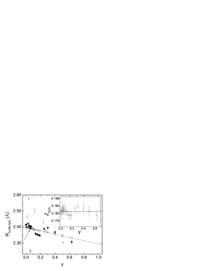
Figure 13: The average distance between Cu/Ni and apical oxygen atom in LSCNO with various Ni content, $y$. The solid circles mark the direct results of Rietveld refinement procedure while the open circles denote the same results with the assumption that $z_{\text{O(2)}}=0.181$ Å= const. The solid line is the linear interpolation of the results marked as open circles. The small open triangles mark the data from Ref. [Wu et al., 1996], the large solid diamond - the value of $R_{\text{Cu-O(2)}}$ from Ref. [Radaelli et al., 1994], and the open star - $R_{\text{Ni-O(2)}}($y$=0.06)$ from Ref. [Haskel et al., 2001]. The arrow indicates $R_{\text{Cu/Ni-O(2)}}($y$=0.06)$, marked as the solid star and calculated as described in the text. Inset: the refined $z$ coordinate of O(2) apical atom. The solid line marks the value 0.181.

The X-ray diffraction measurements are not light-atoms sensitive; therefore the uncertainties of $z_{\text{{O(2)}}}$ are relative large. Within the error margins, there are no obvious trend in the $z_{\text{{O(2)}}}$ vs $y$ dependence and $z_{\text{{O(2)}}}$ can be accepted as being constant and equal to 0.181(3) in the whole investigated doping range. The uncertainties in the determined $z_{\text{{O(2)}}}$ are transferred onto the calculated average interatomic Cu/Ni-O(2) distances, $R_{\text{{Cu/Ni-O(2)}}}\equiv R_{\text{O(2)}}$. Thus, the found $R_{\text{O(2)}}$ vs $y$ behavior mimics $z_{\text{{O(2)}}}$ vs $y$ dependence, as it can be clearly seen in the main panel of Fig. 13. However, taking $z_{\text{{O(2)}}}$=const as granted results in smooth linear dependence of $R_{\text{O(2)}}$ vs $y$ (see open circles in Fig. 13) that mimics linear decrease of $c$ with increasing $y$. This means that within the error margins our measurements do not reveal a nonmonotonic $R_{\text{O(2)}}$ vs $y$ behavior observed in Ref. [Wu et al., 1996]. As mentioned in Sec. III.1, XPD is not atom-specific in the sense that only averaged Cu/Ni-O(2) distance is measured. For a given $y$, this measured $R_{\text{{O(2)}}}$ distance can be expressed as $y\cdot R_{\text{{Ni-O(2)}}}+(1-y)\cdot R_{\text{{Cu-O(2)}}}$, where $R_{\text{{Ni-O(2)}}}$ ($R_{\text{{Cu-O(2)}}}$) is Ni-O(2) [Cu-O(2)] distance, respectively. $R_{\text{O(2)}}$ for $y$=0.06 can be calculated in this way with the use of $R_{\text{{Ni-O(2)}}}$=2.250(12) Å obtained for this Ni content by Haskel et al. from EXAFS spectra (Ref. [Haskel et al., 2001]) and $R_{\text{{Cu-O(2)}}}$=2.397(5) Å  from our XPD measurements for undoped ($y$=0) structure. The calculated $R_{\text{O(2)}}$($y$=0.06)=2.392 Å  is in perfect agreement with the value 2.391 Å  obtained directly from Rietveld analysis with the assumption that $z_{\text{O(2)}}=0.181$ Å  (see Fig. 13). No significant differences were found in the $R_{\text{{Ni-O(2)}}}$ values for $y\leq 0.07$.Haskel et al. (2001); Hiraka et al. (2009) The linear dependence of $R_{\text{{Cu/Ni-O(2)}}}$ vs $y$, when extrapolated to $y$=1, yields the value that is 0.04 Å  larger than $R_{\text{{Ni-O(2)}}}$($y$=0.06) (see the solid line in Fig. 13). This fact gives some grounds for speculation that $R_{\text{{Ni-O(2)}}}$ may change for $y>0.07$.

Appendix B Scaling analysis

Since the different approaches to the static scaling in SG exist in literature,Dekker et al. (1988); Chou et al. (1995); Geschwind et al. (1990) it is worth to explore them one after the other to check, which of them describes the experimental data in the best way. In the following, we will present the details of scaling analysis for LSCNO25, but we have also carried out the similar analysis for LSCNO17 and LSCNO50.

In the derivation of the Eq. 4 the interactions in the system are assumed to average perfectly to zero.Barbara et al. (1981); Fischer (1975); Suzuki (1977) Since evidently this is not our case and $\theta$ in the CW law describing $\chi_{l}$ of LSCNO has a substantial value, we first tried to follow the approach based on expanding magnetization $M$ in odd powers of $\chi_{l}H$ (instead of $H/T$)Omari et al. (1983); Yeung et al. (1987); Dekker et al. (1988); Gingras et al. (1996)

$$M(T,H)=\chi_{l}H-a_{3}(\chi_{l}H)^{3}+a_{5}(\chi_{l}H)^{5}-a_{7}(\chi_{l}H)^{7}+...,$$ (14)

The coefficients $a_{3}$, $a_{5}$,… here are $T$-dependent. Since now $\chi_{l}$ has not a simple Curie form, $\chi_{l}\propto 1/T$, the scaling described by Eq. (4) is replaced by the following relationshipDekker et al. (1988)

$$\frac{\chi_{nl}}{\mid t\mid^{\beta}}=g_{\mp}\left(\frac{\chi_{l}H}{|t|^{\frac{\beta+\gamma}{2}}}\right),$$ (15)

where $g_{-}$ and $g_{+}$ is another pair of the scaling functions.

Since both pair of scaling functions, $f_{\mp}(x)$ from Eq. (4) and $g_{\mp}(x)$ from Eq. (15), behave as const$\cdot x^{2/\delta}$ in the large-$x$ limit, Chalupa (1977); Barbara et al. (1981); Dekker et al. (1988) the same value $\delta$=5.8$\pm$0.1 found from the power dependence of $\chi_{nl}$ vs $H$ at $T_{g}$ (Eq. (5); see also the inset to Fig. 9) is used in both scalings to calculate $\gamma$ from the adjusted $\beta$ [Eq. (6)]. To perform scaling according to Eq. (15), $\beta$ is adjusted in such a way that coincidence of the data on two curves in $\chi_{nl}/|t|^{\beta}$ vs $\chi_{l}H/|t|^{(\beta+\gamma)/2}$ plot is as good qualitatively as possible. The best results have been obtained for $\beta$=0.75 and $\gamma$=3.6. As it is seen in Fig.14, the quality of the scaling is not satisfactory.

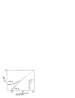
Figure 14: (Color online) Scaling plot for LSCNO25 according to Eq. (15) with $\beta$=0.75 and $\gamma$=3.6 for the nonlinear susceptibility $\chi_{nl}$ at various magnetic fields from 0.1 T to 5 T at temperatures below ($t$$<$0) and above ($t$$>$0) $T_{g}$=10.2 K.

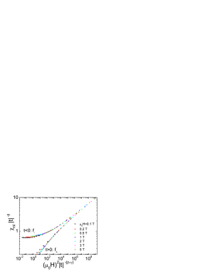
Figure 15: (Color online) Scaling plot for the nonlinear susceptibility $\chi_{nl}$ of LSCNO25 according to Eq. (4) with $\beta$=0.75 and $\gamma$=3.6 and at the same fields and temperatures as in Fig. 14.

To improve the quality of scaling we have employed Eq. (4). The best collapse of the data onto the two universal curves has been obtained once again for $\beta$=0.75 with the uncertainty estimated to be $\sim$0.05. This implies $\gamma$=3.6$\pm$0.3. The resulting scaling is shown in Fig.15. The quality of scaling is much better than this obtained by employing Eq. (15) and almost perfect for fields larger than 0.2 T. Thus, this form of scaling [i.e. given by Eq. (4)] is used for LSCNO.

However, while the log-log plots presented in Figs. 14 and 15 are enough to make direct comparison between the quality of obtained the best scalings according to Eq. (15) or Eq. (4), to estimate the critical temperature region where the scaling is valid, it is better to use Eq. (7), in which the argument of the scaling function is linear in $t$, as described in Sec. IV.1.

References

- (1)
- Bishop (2004) A. R. Bishop, J. Phys. Chem. Solids 65, 1449 (2004)
- Wu and Leighton (2003) J. Wu and C. Leighton, Phys. Rev. B 67, 174408 (2003)
- Phan et al. (2004) M.-H. Phan, T.-L. Phan, T.-N. Huynh, S.-C. Yu, J. R. Rhee, N. V. Khiem, and N. X. Phuc, J. Appl. Phys. 95, 7531 (2004)
- Salamon and Jaime (2001) M. B. Salamon and M. Jaime, Rev. Mod. Phys. 73, 583 (2001)
- Laiho et al. (2001) R. Laiho, E. Lähderanta, J. Salminen, K. G. Lisunov, and V. S. Zakhvalinskii, Phys. Rev. B 63, 094405 (2001)
- Lander et al. (1991) G. H. Lander, P. J. Brown, C. Stassis, P. Gopalan, J. Spalek, and G. Honig, Phys. Rev. B 43, 448 (1991)
- Freeman et al. (2006) P. G. Freeman, A. T. Boothroyd, D. Prabhakaran, and J. Lorenzana, Phys. Rev. B 73, 014434 (2006)
- Chou et al. (1995) F. C. Chou, N. R. Belk, M. A. Kastner, R. J. Birgeneau, and A. Aharony, Phys. Rev. Lett. 75, 2204 (1995)
- Niedermayer et al. (1998) C. Niedermayer, C. Bernhard, T. Blasius, A. Golnik, A. Moodenbaugh, and J. I. Budnick, Phys. Rev. Lett. 80, 3843 (1998)
- Dagotto (2005) E. Dagotto, Science 309, 257 (2005)
- Hasselmann et al. (2004) N. Hasselmann, A. H. C. Neto, and C. M. Smith, Phys. Rev. B 69, 014424 (2004)
- Alloul et al. (2009) H. Alloul, J. Bobroff, M. Gabay, and P. J. Hirschfeld, Rev. Mod. Phys. 81, 45 (2009), and references therein.
- Julien (2003) M.-H. Julien, Physica B 329-333, 693 (2003), ISSN 0921-4526, and references therein.
- Mitrović et al. (2008) V. F. Mitrović, M.-H. Julien, C. de Vaulx, M. Horvati, C. Berthier, T. Suzuki, and K. Yamada, Phys. Rev. B 78, 014504 (2008)
- Panagopoulos and Dobrosavljević (2005) C. Panagopoulos and V. Dobrosavljević, Phys. Rev. B 72, 014536 (2005)
- Raičević et al. (2008) I. Raičević, J. Jaroszyski, D. Popović, C. Panagopoulos, and T. Sasagawa, Phys. Rev. Lett. 101, 177004 (2008)
- Zhang and Rice (1988) F. C. Zhang and T. M. Rice, Phys. Rev. B 37, 3759 (1988)
- Aharony et al. (1988) A. Aharony, R. J. Birgeneau, A. Coniglio, M. A. Kastner, and H. E. Stanley, Phys. Rev. Lett. 60, 1330 (1988)
- Kivelson et al. (2003) S. A. Kivelson, I. P. Bindloss, E. Fradkin, V. Oganesyan, J. M. Tranquada, A. Kapitulnik, and C. Howald, Rev. Mod. Phys. 75, 1201 (2003)
- Lüscher et al. (2006) A. Lüscher, G. Misguich, A. I. Milstein, and O. P. Sushkov, Phys. Rev. B 73, 085122 (2006)
- Cho et al. (1992) J. H. Cho, F. Borsa, D. C. Johnston, and D. R. Torgeson, Phys. Rev. B 46, 3179 (1992)
- Sanna et al. (2010) S. Sanna, F. Coneri, A. Rigoldi, G. Concas, S. R. Giblin, and R. De Renzi, Phys. Rev. B 82, 100503 (2010)
- Coneri et al. (2010) F. Coneri, S. Sanna, K. Zheng, J. Lord, and R. De Renzi, Phys. Rev. B 81, 104507 (2010)
- Yang et al. (2009) J. Yang, J. Hwang, E. Schachinger, J. P. Carbotte, R. P. S. M. Lobo, D. Colson, A. Forget, and T. Timusk, Phys. Rev. Lett. 102, 027003 (2009)
- Panagopoulos et al. (2002) C. Panagopoulos, J. L. Tallon, B. D. Rainford, T. Xiang, J. R. Cooper, and C. A. Scott, Phys. Rev. B 66, 064501 (2002)
- Panagopoulos et al. (2004) C. Panagopoulos, A. P. Petrovic, A. D. Hillier, J. L. Tallon, C. A. Scott, and B. D. Rainford, Phys. Rev. B 69, 144510 (2004)
- Sachdev (2010) S. Sachdev, Phys. Status Solidi B 247, 537 (2010)
- Mendels et al. (1994) P. Mendels, H. Alloul, J. H. Brewer, G. D. Morris, T. L. Duty, S. Johnston, E. J. Ansaldo, G. Collin, J. F. Marucco, C. Niedermayer, et al., Phys. Rev. B 49, 10035 (1994)
- Zaanen and Gunnarsson (1989) J. Zaanen and O. Gunnarsson, Phys. Rev. B 40, 7391 (1989)
- Machida (1989) K. Machida, Physica C 158, 192 (1989)
- Schultz (1989) H. J. Schultz, J. Phys.(Paris) 50, 2833 (1989)
- Hayden et al. (1992) S. M. Hayden, G. H. Lander, J. Zarestky, P. J. Brown, C. Stassis, P. Metcalf, and J. M. Honig, Phys. Rev. Lett. 68, 1061 (1992)
- Tranquada et al. (1995) J. M. Tranquada, B. J. Sternlieb, J. D. Axe, Y. Nakamura, and S. Uchida, Nature 375, 561 (1995)
- Freeman et al. (2004) P. G. Freeman, A. T. Boothroyd, D. Prabhakaran, M. Enderle, and C. Niedermayer, Phys. Rev. B 70, 024413 (2004)
- Pines (1997) D. Pines, Physica C 282-287, 273 (1997), and references herein
- Mendels et al. (1999) P. Mendels, J. Bobroff, G. Collin, H. Alloul, M. Gabay, J. F. Marucco, N. Blanchard, and B. Grenier, Europhys. Lett. 46, 678 (1999)
- Kofu et al. (2005) M. Kofu, H. Kimura, and K. Hirota, Phys. Rev. B 72, 064502 (2005)
- Xiao et al. (1990) G. Xiao, M. Z. Cieplak, J. Q. Xiao, and C. L. Chien, Phys. Rev. B 42, 8752 (1990)
- Nakano et al. (1998) T. Nakano, N. Momono, T. Nagata, M. Oda, and M. Ido, Phys. Rev. B 58, 5831 (1998)
- Hudson et al. (2001) E. W. Hudson, K. M. Lang, V. Madhavan, S. H. Pan, H. Eisaki, S. Uchida, and J. C. Davis, Nature 411, 920 (2001)
- Pimenov et al. (2005) A. V. Pimenov, A. V. Boris, L. Yu, V. Hinkov, T. Wolf, J. L. Tallon, B. Keimer, and C. Bernhard, Phys. Rev. Lett. 94, 227003 (2005)
- Hiraka et al. (2009) H. Hiraka, D. Matsumura, Y. Nishihata, J. Mizuki, and K. Yamada, Phys. Rev. Lett. 102, 037002 (2009)
- Paszkowicz (2005) W. Paszkowicz, Nucl. Instrum. Meth. A 551, 162 (2005)
- Rodriguez-Carvajal (2001) J. Rodriguez-Carvajal, Newslett. IUCr Commission Powd. Diffr. 26, 12 (2001)
- Wu et al. (1996) X. Wu, S. Jiang, F. Pan, J. Lin, N. Xu, Z. Yuheng, X. Gaoji, and M. Zhiqiang, Physica C 271, 331 (1996)
- Zhiqiang et al. (1998) M. Zhiqiang, X. Gaojie, Y. Hongjie, W. Bin, Q. Xueyin, and Z. Yuheng, Phys. Rev. B 58, 15116 (1998)
- Haskel et al. (2001) D. Haskel, E. A. Stern, V. Polinger, and F. Dogan, Phys. Rev. B 64, 104510 (2001)
- (49) R. Minikayev et al.; unpublished
- Marcano et al. (2007) N. Marcano, J. C. G. Sal, J. I. Espeso, L. F. Barquín, and C. Paulsen, Phys. Rev. B 76, 224419 (2007)
- K rner et al. (2000) S. K rner, A. Weber, J. Hemberger, E.-W. Scheidt, and G. R. Stewart, J. Low. Temp. Phys 121, 1573 (2000)
- Johnston (1989) D. C. Johnston, Phys. Rev. Lett. 62, 957 (1989)
- Malinowski et al. (2010) A. Malinowski, V. L. Bezusyy, R. Minikayev, W. Paszkowicz, P. Dziawa, Y. Syryanny, and M. Sawicki, Acta Phys. Pol. A 118, 244 (2010), V. L. Bezusyy, A. Malinowski, R. Minikayev, W. Paszkowicz, P. Dziawa, and R. Gorzelniak, ibid. 118, 402 (2010)
- Ishikawa et al. (1992) N. Ishikawa, N. Kuroda, H. Ikeda, and R. Yoshizaki, Physica C 203, 284 (1992)
- Süllow et al. (1997) S. Süllow, G. J. Nieuwenhuys, A. A. Menovsky, J. A. Mydosh, S. A. M. Mentink, T. E. Mason, and W. J. L. Buyers, Phys. Rev. Lett. 78, 354 (1997)
- Mulder et al. (1982) C. A. M. Mulder, A. J. van Duyneveldt, and J. A. Mydosh, Phys. Rev. B 25, 515 (1982)
- Fisher and Huse (1986) D. S. Fisher and D. A. Huse, Phys. Rev. Lett. 56, 1601 (1986)
- Giot et al. (2008) M. Giot, A. Pautrat, G. André, D. Saurel, M. Hervieu, and J. Rodriguez-Carvajal, Phys. Rev. B 77, 134445 (2008)
- Pytte and Imry (1987) E. Pytte and Y. Imry, Phys. Rev. B 35, 1465 (1987)
- Binder and Young (1986) K. Binder and A. P. Young, Rev. Mod. Phys. 58, 801 (1986)
- J. L. Dormann and Fiorani (1988) L. B. J. L. Dormann and D. Fiorani, J. Phys. C: Solid State Phys. 21, 2015 (1988)
- Néel (1949) L. Néel, Ann. Geophys. 5, 99 (1949)
- Brown (1963) W. F. Brown, Phys. Rev. 130, 1677 (1963)
- Mulder et al. (1981) C. A. M. Mulder, A. J. van Duyneveldt, and J. A. Mydosh, Phys. Rev. B 23, 1384 (1981), To compare the numerical values note that in this Ref. and in some others as well, a log is used in the definition of the parameter , not ln.
- Mydosh (1993) J. A. Mydosh, Spin glasses: An experimental introduction (Taylor & Francis Ltd., London, 1993)
- Li et al. (2005) D. X. Li, T. Yamamura, S. Nimori, K. Yubuta, and Y. Shiokawa, Appl.Phys. Lett. 87, 142505 (2005)
- Tien et al. (2000) C. Tien, C. H. Feng, C. S. Wur, and J. J. Lu, Phys. Rev. B 61, 12151 (2000)
- Bean and Livingston (1959) C. P. Bean and J. D. Livingston, J. Appl. Phys. 30, S120 (1959)
- Westerholt et al. (1986) K. Westerholt, I. Abs-Wurmbach, and R. Dahlbeck, Phys. Rev. B 34, 6437 (1986)
- Morgownik and Mydosh (1981) A. F. J. Morgownik and J. A. Mydosh, Phys. Rev. B 24, 5277 (1981)
- Morgownik and Mydosh (1982) A. F. J. Morgownik and J. A. Mydosh, J. Appl. Phys. 53, 2211 (1982)
- Morgownik et al. (1984) A. F. J. Morgownik, J. A. Mydosh, and C. L. Foiles, Phys. Rev. B 29, 4144 (1984)
- Rao et al. (1983) K. V. Rao, M. Fähnle, E. Figueroa, O. Beckman, and L. Hedman, Phys. Rev. B 27, 3104 (1983)
- V. Degiorgio and T.Bellini (1990) F. V. Degiorgio, R. Piazza and T.Bellini, J. Phys.: Condens. Matter 2, 2 SA69 (1990), and the references cited herein.
- (75) For the very interesting history of using the stretched exponential function in different fields see: M. Cardona et al., Ann. Phys. (Leipzig) , 842 (2007).
- Lois et al. (2009) G. Lois, J. Blawzdziewicz, and C. S. O’Hern, Phys. Rev. Lett. 102, 015702 (2009)
- Phillips (1996) J. C. Phillips, Rep. Prog. Phys. 59, 1133 (1996)
- Böhmer et al. (1993) R. Böhmer, K. L. Ngai, C. A. Angell, and D. J. Plazek, J. Chem. Phys. 99, 4201 (1993)
- Phillips (2006) J. C. Phillips, Phys. Rev. B 73, 104206 (2006)
- Jund et al. (2001) P. Jund, R. Jullien, and I. Campbell, Phys. Rev. E 63, 036131 (2001)
- Continentino and Malozemoff (1986) M. A. Continentino and A. P. Malozemoff, Phys. Rev. B 33, 3591 (1986)
- Ogielski (1985) A. T. Ogielski, Phys. Rev. B 32, 7384 (1985)
- C. De Dominicis and Lainee (1985) H. O. C. De Dominicis and F. Lainee, J. Phys. (Paris) Lett. 46, L463 (1985)
- Hoogerbeets et al. (1985) R. Hoogerbeets, W.-L. Luo, and R. Orbach, Phys. Rev. Lett. 55, 111 (1985)
- G. Sinha and Majumdar (1996) M. U. G. Sinha, R. Chatterjee and A. K. Majumdar, J. Magn. Magn. Mat. 164, 345 (1996)
- Patel et al. (2002) R. S. Patel, D. Kumar, and A. K. Majumdar, Phys. Rev. B 66, 054408 (2002)
- Kinzel (1979) W. Kinzel, Phys. Rev. B 19, 4595 (1979)
- Guy (1977) C. N. Guy, J. Phys. F: Met. Phys. 7, 1505 (1977)
- Guy (1978) C. N. Guy, J. Phys. F: Met. Phys. 8, 1309 (1978)
- Dhar et al. (2003) S. Dhar, O. Brandt, A. Trampert, K. J. Friedland, Y. J. Sun, and K. H. Ploog, Phys. Rev. B 67, 165205 (2003)
- Smith et al. (1994) M. Smith, A. Dissanayake, and H. X. Jiang, Phys. Rev. B 49, 4514 (1994)
- Tiwari and Rajeev (2005) S. D. Tiwari and K. P. Rajeev, Phys. Rev. B 72, 104433 (2005)
- Campbell (1986) I. A. Campbell, Phys. Rev. B 33, 3587 (1986)
- Campbell (1988) I. A. Campbell, Phys. Rev. B 37, 9800 (1988)
- Chamberlin et al. (1984) R. V. Chamberlin, G. Mozurkewich, and R. Orbach, Phys. Rev. Lett. 52, 867 (1984)
- Fischer (1975) K. H. Fischer, Phys. Rev. Lett. 34, 1438 (1975)
- Sherrington and Kirkpatrick (1975) D. Sherrington and S. Kirkpatrick, Phys. Rev. Lett. 35, 1792 (1975)
- Widom (1965) B. Widom, J. Chem. Phys. 43, 3898 (1965)
- Kadanoff (1966) L. P. Kadanoff, Physics 2, 263 (1966)
- Fischer and Hertz (1991a) K. H. Fischer and J. Hertz, Spin glasses (Cambridge University Press, Cambridge, 1991a)
- Chalupa (1977) J. Chalupa, Solid State Commun. 22, 315 (1977)
- Suzuki (1977) M. Suzuki, Prog. Theor. Phys. 58, 1151 (1977)
- Omari et al. (1983) R. Omari, J. J. Prejean, and J. Souletie, J. Phys. (Paris) 44, 1069 (1983)
- Dekker et al. (1988) C. Dekker, A. F. M. Arts, and H. W. de Wijn, Phys. Rev. B 38, 8985 (1988)
- Fischer and Hertz (1991b) K. H. Fischer and J. Hertz, Spin glasses (Cambridge University Press, Cambridge, 1991b), chap. 8
- Beauvillain et al. (1984) P. Beauvillain, C. Dupas, J. P. Renard, and P. Veillet, Phys. Rev. B 29, 4086 (1984), and references therein.
- Barbara et al. (1981) B. Barbara, A. P. Malozemoff, and Y. Imry, Phys. Rev. Lett. 47, 1852 (1981)
- Malozemoff et al. (1983) A. P. Malozemoff, S. E. Barnes, and B. Barbara, Phys. Rev. Lett. 51, 1704 (1983)
- Geschwind et al. (1990) S. Geschwind, D. A. Huse, and G. E. Devlin, Phys. Rev. B 41, 2650 (1990)
- Edwards and Anderson (1975) S. F. Edwards and P. W. Anderson, J. Phys. F. 5, 965 (1975)
- Sherrington and Southern (1975) D. Sherrington and B. W. Southern, J. Phys. F 5, L49 (1975)
- Kirkpatrick and Sherrington (1978) S. Kirkpatrick and D. Sherrington, Phys. Rev. B 17, 4384 (1978)
- Patterson et al. (1978) J. D. Patterson, G. R. Gruzalski, and D. J. Sellmyer, Phys. Rev. B 18, 1377 (1978)
- Korenblit and Shender (1985) I. Y. Korenblit and E. F. Shender, Sov. Phys. JETP 62, 1030 (1985)
- Takayama (1988) H. Takayama, Prog. Theor. Phys. 80, 827 (1988)
- Fyodorov et al. (1987) Y. V. Fyodorov, I. Y. Korenblit, and E. F. Shender, J. Phys. C: Solid State Phys. 20, 1835 (1987)
- Hohenberg and Halperin (1977) P. C. Hohenberg and B. I. Halperin, Rev. Mod. Phys. 49, 435 (1977)
- Wang et al. (2004) F. Wang, J. Zhang, Y.-f. Chen, G.-j. Wang, J.-r. Sun, S.-y. Zhang, and B.-g. Shen, Phys. Rev. B 69, 094424 (2004)
- Vijayanandhini et al. (2009) K. Vijayanandhini, C. Simon, V. Pralong, V. Caignaert, and B. Raveau, Phys. Rev. B 79, 224407 (2009)
- Gunnarsson et al. (1988) K. Gunnarsson, P. Svedlindh, P. Nordblad, L. Lundgren, H. Aruga, and A. Ito, Phys. Rev. Lett. 61, 754 (1988)
- Mukadam et al. (2005) M. D. Mukadam, S. M. Yusuf, P. Sharma, S. K. Kulshreshtha, and G. K. Dey, Phys. Rev. B 72, 174408 (2005)
- Mathieu et al. (2005) R. Mathieu, A. Asamitsu, Y. Kaneko, J. P. He, and Y. Tokura, Phys. Rev. B 72, 014436 (2005)
- Tholence (1980) J. L. Tholence, Solid State Commun. 35, 113 (1980)
- Souletie and Tholence (1985) J. Souletie and J. L. Tholence, Phys. Rev. B 32, 516 (1985)
- Shtrikman and Wohlfarth (1981) S. Shtrikman and E. P. Wohlfarth, Phys. Lett. A 85, 467 (1981)
- Birgeneau et al. (1988) R. J. Birgeneau, D. R. Gabbe, H. P. Jenssen, M. A. Kastner, P. J. Picone, T. R. Thurston, G. Shirane, Y. Endoh, M. Sato, K. Yamada, et al., Phys. Rev. B 38, 6614 (1988)
- Kofu et al. (2009) M. Kofu, S.-H. Lee, M. Fujita, H.-J. Kang, H. Eisaki, and K. Yamada, Phys. Rev. Lett. 102, 047001 (2009)
- Adachi et al. (2008) T. Adachi, N. Oki, Risdiana, S. Yairi, Y. Koike, and I. Watanabe, Phys. Rev. B 78, 134515 (2008)
- Adachi et al. (2004) T. Adachi, S. Yairi, Y. Koike, I. Watanabe, and K. Nagamine, Phys. Rev. B 70, 060504 (2004)
- Tsutsui et al. (2009) K. Tsutsui, A. Toyama, T. Tohyama, and S. Maekawa, Phys. Rev. B 80, 224519 (2009)
- (131) For a condensed review of the recent experimental results see: M.-H. Julien, Physica B, 329-333, 693 (2003).
- Nordblad (2004) P. Nordblad, J. Phys.: Condens. Matter 16, S715 (2004)
- Mattsson et al. (1995) J. Mattsson, T. Jonsson, P. Nordblad, H. Aruga Katori, and A. Ito, Phys. Rev. Lett. 74, 4305 (1995)
- Lundgren et al. (1982) L. Lundgren, P. Svedlindh, and O. Beckman, Phys. Rev. B 26, 3990 (1982)
- Djurberg et al. (1995) C. Djurberg, J. Mattsson, P. Nordblad, L. Hoines, and J. A. Cowen, J. Magn. Magn. Mater. 140-144, 1721 (1995)
- Lévy (1988) L. P. Lévy, Phys. Rev. B 38, 4963 (1988)
- Ballesteros et al. (2000) H. G. Ballesteros, A. Cruz, L. A. Fernández, V. Martín-Mayor, J. Pech, J. J. Ruiz-Lorenzo, A. Tarancón, P. Téllez, C. L. Ullod, and C. Ungil, Phys. Rev. B 62, 14237 (2000)
- Campbell et al. (2006) I. A. Campbell, K. Hukushima, and H. Takayama, Phys. Rev. Lett. 97, 117202 (2006)
- Hasenbusch et al. (2008) M. Hasenbusch, A. Pelissetto, and E. Vicari, Phys. Rev. B 78, 214205 (2008)
- Campbell and Petit (2010) I. A. Campbell and D. C. M. C. Petit, J. Phys. Soc. Jpn. 79, 011006 (2010), and the references given therein.
- Kawamura (2010) H. Kawamura, J. Phys.: Conf. Ser. 233, 1 (2010)
- Gunnarsson et al. (1991) K. Gunnarsson, P. Svedlindh, P. Nordblad, L. Lundgren, H. Aruga, and A. Ito, Phys. Rev. B 43, 8199 (1991)
- Radaelli et al. (1994) P. G. Radaelli, D. G. Hinks, A. W. Mitchell, B. A. Hunter, J. L. Wagner, B. Dabrowski, K. G. Vandervoort, H. K. Viswanathan, and J. D. Jorgensen, Phys. Rev. B 49, 4163 (1994)
- Yeung et al. (1987) I. Yeung, R. Roshko, and G. Williams, J. Magn. Magn. Mater. 68, 39 (1987)
- Gingras et al. (1996) M. J. P. Gingras, C. V. Stager, B. D. Gaulin, N. P. Raju, and J. E. Greedan, J. Appl. Phys. 79, 6170 (1996)