Renormalization and cyclotron resonance
in bilayer graphene with weak electron-hole asymmetry

Abstract

Cyclotron resonance in bilayer graphene is studied with weak electron-hole asymmetry, suggested by experiment, taken into account and with the focus on many-body corrections that evade Kohn’s theorem. It is shown by direct calculation that the theory remains renormalizable to $O(e^{2})$ in the presence of electron-hole asymmetry parameters, and a general program to carry out renormalization for graphene under a magnetic field is presented. Inclusion of electron-hole asymmetry in part improves the theoretical fit to the existing data and the data appear to indicate the running of the renormalized velocity factor with the magnetic field, which is a key consequence of renormalization.

I Introduction

Graphene NG ; ZTSK ; ZJS ; ZA ; PGN supports charge carriers that behave as Dirac fermions, which, in a magnetic field, lead to a particle-hole symmetric and unequally-spaced pattern of Landau levels. Accordingly, graphene gives rise to a variety of cyclotron resonance, both intraband and interband, with resonance energies varying from one resonance to another. This is in sharp contrast to standard quantum Hall systems with a parabolic energy dispersion, where cyclotron resonance takes place between adjacent Landau levels, hence at a single frequency $\omega_{c}=eB/m^{*}$, which, according to Kohn’s theorem, Kohn is unaffected by electron-electron interactions. The nonparabolic spectra AA in graphene offer the challenge of detecting many-body corrections to cyclotron resonance.

Theoretical studies AFsr ; IWFB ; BMgr ; KCC ; KScr over the past few years have revealed some notable features of quantum corrections to cyclotron resonance in graphene and bilayer NMMKF ; MF graphene. The genuine many-body corrections arise from vacuum polarization, specific to graphene, which diverges logarithmically at short wavelengths. This means that one has to carry out renormalization properly, as in quantum electrodynamics, to extract observable results. In particular, for bilayer graphene it turns out that both the leading intralayer and interlayer coupling strengths undergo renormalization and that their renormalized strengths run with the magnetic field. Bilayer graphene is marked with the unique property that its band gap is externally controllable. OBSHR ; Mc ; CNMPL ; OHL ; Mucha

Experiment has so far verified, via infrared spectroscopy, some basic features of cyclotron resonance in monolayer JHT ; DCN ; HCJL and bilayer HJTS ; OFB graphene. The data for the monolayer show a good symmetry between the electron and hole bands but generally show no clear sign of the many-body effect, except for a datum. JHT Indeed, a comparison between some leading intraband and interband cyclotron resonances revealed a small deviation in excitation energy, consistent with the presence of many-body corrections roughly in magnitude and sign.

The situation is quite different for bilayer graphene, for which only a limited number of data are available so far. The data HJTS on intraband resonances show a weak electron-hole asymmetry, and generally defy a good fit by theory. Actually one has to employ different values of the velocity factor $v$ to fit the electron data and hole data separately.

Earlier Raman Malard spectroscopy and subsequent infrared LHJH ; ZLBF ; KHML spectroscopy of bilayer graphene under zero magnetic field also revealed a significant asymmetry between the conduction and valence bands, mainly due to subleading intra- and inter-layer couplings $\triangle$ and $\gamma_{4}$.

The purpose of this paper is to reexamine cyclotron resonance in bilayer graphene, with possible electron-hole and valley asymmetries taken into account. It is not clear a priori whether the renormalizability of the low-energy effective theory is maintained in the presence of electron-hole asymmetry, since the asymmetry parameters (especially, $\gamma_{4}$) critically modify the ultraviolet structure of the theory. We show that the theory indeed remains renormalizable to $O(e^{2})$ (at least), and that the renormalization counterterms depend on $\gamma_{4}$ in a nontrivial way. We present a general algorithm to carry out renormalization for graphene under a magnetic field, executable even numerically. Inclusion of electron-hole asymmetry parameters partially improves the theoretical fit to the existing data, and the fit in turn suggests some nontrivial modification of the spectra of the zero-mode and pseudo-zero-mode Landau levels specific to bilayer graphene.

In Sec. II we briefly review the effective theory of bilayer graphene and examine the effect of electron-hole and valley asymmetries. In Sec. III we study the Coulombic many-body corrections to cyclotron resonance, with a focus on renormalization and its consequences. Section IV is devoted to a summary and discussion.

II bilayer graphene

Bilayer graphene consists of two coupled honeycomb lattices of carbon atoms, arranged in Bernal $A^{\prime}B$ stacking. The electrons in it are described by four-component spinor fields on the four inequivalent sites $(A,B)$ and $(A^{\prime},B^{\prime})$ in the bottom and top layers, and their low-energy features are governed by the two inequivalent Fermi points $K$ and $K^{\prime}$ in the Brillouin zone. The intralayer coupling $\gamma_{0}\equiv\gamma_{AB}\sim 3$  eV is related to the Fermi velocity $v=(\sqrt{3}/2)\,a_{\rm L}\gamma_{0}/\hbar\sim 10^{6}$ m/s (with $a_{\rm L}=0.246$nm) in monolayer graphene. The interlayer couplings Malard ; ZLBF $\gamma_{1}\equiv\gamma_{A^{\prime}B}\sim 0.4$ eV and $\gamma_{3}\equiv\gamma_{AB^{\prime}}\sim 0.1$ eV are one-order of magnitude weaker than $\gamma_{0}$. Actually, interlayer hopping via the $(A^{\prime},B)$ dimer bonds modifies the intralayer linear spectra to yield quasi-parabolic spectra MF in the low-energy branches $|\epsilon|<\gamma_{1}$.

The bilayer Hamiltonian with the leading intra- and inter-layer couplings $v\propto\gamma_{0}$ and $\gamma_{1}$ lead to electron-hole symmetric spectra. Infrared spectroscopy ZLBF of bilayer graphene, however, has detected some weak asymmetry between the electron and hole bands, such as (i) the energy difference $\triangle\approx 18$ meV between the $A$ and $B$ sublattices within the same layer and (ii) the next-nearest-neighbor interlayer coupling $\gamma_{4}\equiv\gamma_{AA^{\prime}}=\gamma_{BB^{\prime}}\approx 0.04\,\gamma_{0}$.

The effective Hamiltonian with such intra- and inter-layer couplings is written as MF ; NCGP

$$H^{\rm bi} = \!\!\int\!d^{2}{\bf x}\,\Big{[}\Psi^{{\dagger}}\,{\cal H}_{+}\Psi+\tilde{\Psi}^{{\dagger}}\,{\cal H}_{-}\,\tilde{\Psi}\Big{]},$$

$${\cal H}_{+} = \left(\begin{array}[]{cccc}{1\over{2}}u&&v_{4}\,p^{{\dagger}}&v\,p^{{\dagger}}\\ &-{1\over{2}}u&v\,p&v_{4}\,p\\ v_{4}\,p&v\,p^{{\dagger}}&\triangle-{1\over{2}}u&\gamma_{1}\\ v\,p&v_{4}\,p^{{\dagger}}&\gamma_{1}&\triangle+{1\over{2}}u\\ \end{array}\right),$$ (5)

with $p=p_{x}+i\,p_{y}$, $p^{{\dagger}}=p_{x}-i\,p_{y}$. Here $\Psi=(\psi_{A},\psi_{B^{\prime}},\psi_{A^{\prime}},\psi_{B})^{\rm t}$ stands for the electron field at the $K$ valley, with $A$ and $B$ referring to the associated sublattices; $u$ stands for the interlayer bias, which opens a tunable gap OBSHR between the $K$ and $K^{\prime}$ valleys. We ignore the effect of trigonal warping $\propto\gamma_{3}$ which, in a strong magnetic field, causes only a negligibly small level shift. KSbgr We also ignore weak Zeeman coupling and, for conciseness, suppress the electron spin. Our definition of $v_{4}\equiv-(\gamma_{4}/\gamma_{0})\,v$ differs in sign and by factor $v$ from the one ($v_{4}\rightarrow\gamma_{4}/\gamma_{0}$) in the literature Malard ; LHJH ; ZLBF ; NCGP ; this choice is made simply for notational convenience.

The Hamiltonian ${\cal H}_{-}$ at another ($K^{\prime}$) valley is given by ${\cal H}_{+}$ with $(v,v_{4},u)\rightarrow(-v,-v_{4},-u)$, and acts on a spinor of the form $\tilde{\Psi}=(\psi_{B^{\prime}},\psi_{A},\psi_{B},\psi_{A^{\prime}})^{\rm t}$. Note that ${\cal H}_{+}$ is unitarily equivalent to ${\cal H}_{-}$ with the sign of $u$ reversed,

$$U^{{\dagger}}{\cal H}_{+}|_{u}U={\cal H}_{-}|_{-u}$$ (6)

with $U={\rm diag}(1,1,-1,-1)$. This implies that the electronic spectrum at the $K^{\prime}$ valley is obtained from the spectrum at the $K$ valley by reversing the sign of $u$; in particular, the spectra at the two valleys are the same for $u=0$. Nonzero interlayer voltage $u\not=0$ thus acts as a valley-symmetry breaking.

We adopt the set of experimental values ZLBF

$$v \approx 1.1\times 10^{6}\,{\rm m/s},\ \gamma_{1}\approx 404\,{\rm meV},$$

$$v_{4}/v \equiv -\gamma_{4}/\gamma_{0}\approx-0.04,\ \triangle\approx 18\,{\rm meV},$$ (7)

in what follows. Full account is also taken of the effect of interlayer bias $u$. For notational simplicity, however, we often present analytical expressions only for $u=0$.

The Hamiltonian $H^{\rm bi}$ gives rise to four bands with electron and hole spectra, which, for $u=0$, read

$$\epsilon_{4}({\bf p}) = \sqrt{v_{+}^{2}\,{\bf p}^{2}+(\gamma_{+}/2)^{2}}+\gamma_{+}/2,$$

$$\epsilon_{3}({\bf p}) = \sqrt{v_{-}^{2}\,{\bf p}^{2}+(\gamma_{-}/2)^{2}}-\gamma_{-}/2,$$

$$\epsilon_{2}({\bf p}) = -\sqrt{v_{+}^{2}\,{\bf p}^{2}+(\gamma_{+}/2)^{2}}+\gamma_{+}/2,$$

$$\epsilon_{1}({\bf p}) = -\sqrt{v_{-}^{2}\,{\bf p}^{2}+(\gamma_{-}/2)^{2}}-\gamma_{-}/2,$$ (8)

where $v_{\pm}\equiv v\pm v_{4}$ and $\gamma_{\pm}\equiv\gamma_{1}\pm\triangle$. Note that $v_{4}$ and $\triangle$ effectively modify $v$ and $\gamma_{1}$, respectively, in a manner different for electrons and holes; the spectra are electron-hole asymmetric unless $v_{4}=\triangle=0$. These band spectra acquire nonzero valley gaps for $u\not=0$.

Let us place bilayer graphene in a strong uniform magnetic field $B_{z}=-B<0$ normal to the sample plane; we set, in ${\cal H}_{\pm}$, $p\rightarrow\Pi=p+eA$ and $p^{{\dagger}}\rightarrow\Pi^{{\dagger}}$ with $A=A_{x}+iA_{y}=B\,y$, and denote the the magnetic length as $\ell=1/\sqrt{eB}$. It is easily seen that the eigenmodes of ${\cal H}_{+}$ have the structure

$$\Psi_{n}=\Big{(}|n\rangle\,b_{n}^{(1)},|n\!-\!2\rangle\,b_{n}^{(2)},|n\!-\!1\rangle\,b_{n}^{(3)},|n\!-\!1\rangle\,b_{n}^{(4)}\Big{)}^{\rm t}$$ (9)

with $n=0,1,2,\dots$, where only the orbital eigenmodes are shown using the standard harmonic-oscillator basis $\{|n\rangle\}$ (with the understanding that $|n\rangle=0$ for $n<0$). The coefficients ${\bf b}_{n}=(b_{n}^{(1)},b_{n}^{(2)},b_{n}^{(3)},b_{n}^{(4)})^{\rm t}$ for $n=2,3,\dots$ are given by the eigenvectors of the reduced Hamiltonian

$$\hat{\cal H}_{\rm red}=\omega_{c}\,\left(\begin{array}[]{cccc}{1\over{2}}u^{\prime}&&r\sqrt{n}&\sqrt{n}\\ &-{1\over{2}}u^{\prime}&\sqrt{n\!-\!1}&r\sqrt{n\!-\!1}\\ r\sqrt{n}&\sqrt{n\!-\!1}&d-{1\over{2}}u^{\prime}&\gamma^{\prime}\\ \sqrt{n}&r\sqrt{n\!-\!1}&\gamma^{\prime}&d+{1\over{2}}u^{\prime}\\ \end{array}\right),$$ (10)

where

$$\omega_{c}\equiv\sqrt{2}\,v/\ell\approx 36.3\times v[10^{6}{\rm m/s}]\,\sqrt{B[{\rm T}]}\ {\rm meV},$$ (11)

with $v$ measured in units of $10^{6}$m/s and $B$ in tesla, is the characteristic cyclotron energy for monolayer graphene; $r\equiv v_{4}/v=-\gamma_{4}/\gamma_{0}\ (\approx-0.04)$, $\gamma^{\prime}\equiv\gamma_{1}/\omega_{c}$, $d\equiv\triangle/\omega_{c}$ and $u^{\prime}\equiv u/\omega_{c}$.

The energy eigenvalues $\epsilon_{n}$ of $\hat{\cal H}_{\rm red}$ are determined from the secular equation, which, for $u=0$, reads

$$n(n-1)(1-r^{2})^{2}-\Big{[}\gamma^{\prime 2}-d^{2}+c_{n}\,(1\!+r^{2})\Big{]}\,\epsilon^{\prime 2}+(\epsilon^{\prime 2})^{2}$$

$$-c_{n}\,[2\,r\,\gamma^{\prime}-d\,(1+r^{2})]\,\epsilon^{\prime}-2d\,(\epsilon^{\prime})^{3}=0,$$ (12)

with $c_{n}=2n-1$ and $\epsilon^{\prime}\equiv\epsilon_{n}/\omega_{c}$. We first consider the $u=0$ case. Let us denote the four solutions of the secular equation as $\epsilon_{-n}^{-}<\epsilon_{-n}<0<\epsilon_{n}<\epsilon_{n}^{+}$ for each integer $n\geq 2$, so that the index $\pm n$ reflects the sign of the energy eigenvalues. For $n=0$ $H^{\rm bi}$ has an obvious zero eigenvalue $\epsilon_{0}=0$, with the eigenvector ${\bf b}_{0}=(1,0,0,0)^{\rm t}$. For $n=1$ the secular equation (12) is reduced to a cubic equation in $\epsilon^{\prime}$, excluding $\epsilon^{\prime}=0$, and leads to three solutions, which, for the present choice (7) of parameters, are given, e.g., by $\epsilon^{\prime}=(-3.96,0.029,4.29)$ at $B=10$ T; we thus denote the corresponding eigenvalues as $(\epsilon^{-}_{-1},\epsilon_{1},\epsilon^{+}_{1})$. This eigenvalue $\epsilon_{1}$ changes sign if one sets $d\rightarrow-d$ and $r\rightarrow-r$ simultaneously. Thus the assignment of $\epsilon_{\pm 1}$ in general depends on the choice of asymmetry parameters $(v_{4},\triangle)$ and also on the interlayer bias $u$. Actually, for zero bias $u=0$, $\epsilon_{1}$ deviates from zero as $v_{4}$ and $\triangle$ develop. In this sense, the $n=1$ Landau level is a pseudo-zero-mode level while the $n=0$ level is a genuine zero-mode level.

As $u$ is turned on, these $n=(0,\pm 1)$ levels go up or down oppositely at the two valleys; e.g., $\epsilon_{0}|_{K}=-\epsilon_{0}|_{K^{\prime}}=u/2$. Their spectra vary linearly with $u$ while other levels $(|n|\geq 2)$ get shifted only slightly. Interestingly, for $0<|u|\ll\omega_{c}$, $\epsilon_{1}\gtrsim\epsilon_{0_{+}}$ at one valley while $\epsilon_{|n|=1}$ at another valley crosses fnx $\epsilon_{0_{+}}$ from below with increasing magnetic field $B$. A nonzero $u$ thus critically spoils the valley symmetry of the $n=(0,\pm 1)$ sector.

The spectra $\epsilon^{+}_{n}$ and $\epsilon^{-}_{-n}$ with $n\geq 1$ form the high-energy branches of the electron and hole Landau levels, respectively; $|\epsilon^{\pm}|\gtrsim\gamma_{1}$. Let us combine $\epsilon_{\pm n}$ into the low-energy branch of Landau levels $\{\epsilon_{n}\}=\{\dots,\epsilon_{-3},\epsilon_{-2},\epsilon_{0},\epsilon_{1},\epsilon_{2},\dots\}$, and denote the three branches $(\epsilon_{-n}^{-},\epsilon_{n},\epsilon_{n}^{+})$ as

$$\epsilon_{n}=\omega_{c}\,\eta_{n}(\gamma^{\prime},d,r,u^{\prime}),\ \epsilon^{\pm}_{n}=\omega_{c}\,\eta^{\pm}_{n}(\gamma^{\prime},d,r,u^{\prime}).$$ (13)

These $(\eta_{n},\eta^{\pm}_{n})\sim\epsilon^{\prime}$ are uniquely determined from $\hat{\cal H}_{\rm red}$ of Eq. (10) or from Eq. (12) as functions of $(\gamma^{\prime},d,r,u^{\prime})$. One can thereby construct the associated eigenvectors, which, e.g., for $u=0$ and $|n|\geq 1$, read ${\bf b}_{n}=(b_{n}^{(1)},b_{n}^{(2)},b_{n}^{(3)},b_{n}^{(4)})^{\rm t}=b_{n}^{(1)}\,(1,\beta_{n}^{(2)},\beta_{n}^{(3)},\beta_{n}^{(4)})^{\rm t}$ with

$$\beta_{n}^{(3)} = -{|n|-\eta_{n}\,(\eta_{n}-d)+(|n|-1)\,r^{2}\over{\sqrt{|n|}\,G_{n}}},$$

$$\beta_{n}^{(4)} = \Big{[}\gamma^{\prime}\,\eta_{n}+(2|n|-1)\,r\Big{]}/\Big{(}\sqrt{|n|}\,G_{n}\Big{)},$$

$$\beta_{n}^{(2)} = \sqrt{|n|-1}\,(\beta_{n}^{(3)}+r\,\beta_{n}^{(4)})/\eta_{n},$$ (14)

where $G_{n}=\gamma^{\prime}+r\,\{\eta_{n}-d+(|n|-1)\,(1-r^{2})/\eta_{n}\}$ and $b_{n}^{(1)}=1/\sqrt{1+\sum_{i=2,3,4}(\beta_{n}^{(i)})^{2}}$. These expressions are equally valid for eigenvectors belonging to $\epsilon_{n}^{\pm}$, with $\eta_{n}\rightarrow\eta_{n}^{\pm}$.

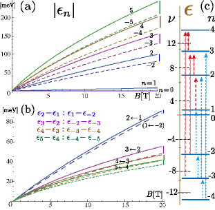
Figure 1: The $3\leftarrow-2$ (or $2\leftarrow-3$) resonance (a) Landau levels as a function of magnetic field $B$ for $\gamma_{1}=404$ meV, $\triangle=18$ meV, $v_{4}/v=-0.04$ and $u=0$; $\epsilon_{n}$ for electrons (solid curves) and $-\epsilon_{-n}$ for holes (dashed curves). (b) Landau gaps for electrons (solid curves) and holes (dashed curves). (c) Typical channels of cyclotron resonance for $u=0$; circularly polarized light can distinguish between the two classes of transitions indicated by different types of arrows.

The Landau-level spectrum $\epsilon_{n}=\omega_{c}\,\eta_{n}(\gamma^{\prime},d,r,u^{\prime})$ depends on the magnetic field $B$ in a nontrivial manner through the dimensionless quantities $\gamma^{\prime}$, $d$ and $u^{\prime}$. Actually, for the choice of $\gamma_{1}=404$ meV, $\triangle=18$ meV, $r=-0.04$ and $u=0$, the electron and hole spectra differ considerably, as shown in Fig. 1. In particular, the zero-mode level $(n=0)$ remains intact while the pseudo-zero-mode level ($n=1$) gets shifted, e.g., by $\sim$ 8 meV as $B$ is increased from 0 to 20 T. The Landau gaps are generally larger for electrons than holes; this is readily understood from the behavior of $\epsilon_{3}({\bf p})\approx(v_{-}^{2}/\gamma^{\prime}_{-})\,{\bf p}^{2}$ for ${\bf p}\rightarrow 0$, which implies that the effective mass $m^{*}\sim\gamma_{-}/(2\,v_{-}^{2})$ is smaller for electrons. The asymmetry between the electron Landau levels $L_{n}$ and hole levels $L_{-n}$ becomes more prominent for higher levels $|n|\geq 2$.

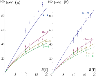
Figure 2: Landau gaps in Fig. 1 (b), compared with the experimental data in Ref. HJTS, on cyclotron resonance energies. (a) Electron band. (b) Hole band.

Cyclotron resonance in bilayer graphene is governed by the selection rule AFsr $\triangle|n|=\pm 1$, and there are two classes of transitions, (i) $L_{\pm(n-1)}\leftarrow L_{-n}$ and (ii) $L_{n}\leftarrow L_{\pm(n-1)}$ (with $n\geq 2$), which are distinguished by the use of circularly-polarized light. See Fig. 1 (c).

As for experiment, Henriksen et al. HJTS measured, via infrared spectroscopy, cyclotron resonance in bilayer graphene in magnetic fields up to 18T. They observed intraband resonances, which are identified with the $L_{2}\leftarrow L_{1}$, $L_{3}\leftarrow L_{2}$, $L_{4}\leftarrow L_{3}$ and $L_{5}\leftarrow L_{4}$ transitions at filling factor $\nu$= 4, 8, 12 and 16, respectively, and the corresponding hole resonances at $\nu$= -4, -8, -12 and -16, together with a significant asymmetry between the electron and hole data.

Such data from Ref. HJTS, are reproduced in Fig. 2. Also included are the zeroth-order Landau gaps of Fig. 1 (b), which apparently fit the experimental data reasonably well, except for the $\nu=4$ electron data on the $L_{2}\leftarrow L_{1}$ resonance, which deviates considerably.

It is worth discussing the effect of interlayer bias $u$ here. The $n=(0,1)$ levels are very sensitive to $u$ and may easily acquire valley gaps for $u\not=0$ while other levels $|n|\geq 2$ are relatively inert as long as $|u|\ll\omega_{c}$. Cyclotron resonances involving the $n=1$ level, i.e., $(1\leftarrow-2)$ and $(2\leftarrow 1)$ resonances, therefore tend to be affected by $u$. Actually, with $u\sim 20\,{\rm meV}$ one can apparently fit the data for those resonances at one valley. The asymmetry, however, is reversed at another valley. Nonzero $u$ may thus broaden the observed widths of the $(1\leftarrow-2)$ and $(2\leftarrow 1)$ resonances but would not account for their asymmetry.

It is clear now that one should treat those resonances separately from the rest of the resonances, which are barely sensitive to $|u|\ll\omega_{c}$. The former and latter are also different in their sensitivities to electron-hole asymmetry $\propto\triangle$ and $v_{4}$. See Fig. 1 (b) again. It shows that for $u=0$ the $2\leftarrow 1$ and $1\leftarrow-2$ gaps barely differ while other Landau gaps exhibit significant asymmetry between the electron and hole bands. In this sense, Fig. 2 shows us that $\triangle\approx 18$meV and $v_{4}\approx-0.04\,v$, obtained from independent experiments, account for the electron-hole asymmetry between the $\nu=(8,12,16)$ data and the $\nu=(-8,-12,-16)$ data reasonably well. It is a nontrivial fact that this single set of parameters can fit the electron and hole data simultaneously.

Poor fitting to the $\nu=4$ data, on the other hand, would suggest that the spectrum of the pseudo-zero-mode level $(|n|=1)$ is further modified AbCh by some other sources. Actually it is expected theoretically BCNM ; KSpzm ; CLBM that the $n=(0,\pm 1)$ sector of bilayer graphene has nontrivial dynamics due to orbital mixing and supports characteristic collective excitations, orbital pseudospin waves. It would be interesting to study how the electron-hole asymmetry affects the detailed structure of this special sector.

III Cyclotron resonance and many-body corrections

In this section we study the many-body corrections to cyclotron resonance, with emphasis on how to carry out renormalization. The Coulomb interaction is written as

$$H^{\rm Coul}={1\over{2}}\sum_{\bf p}v_{\bf p}\,:\rho_{\bf-p}\,\rho_{\bf p}:,$$ (15)

where $\rho_{\bf p}$ is the Fourier transform of the electron density $\rho=\Psi^{{\dagger}}\Psi+\tilde{\Psi}^{{\dagger}}\tilde{\Psi}$; $v_{\bf p}=2\pi\alpha/(\epsilon_{\rm b}|{\bf p}|)$ is the Coulomb potential with $\alpha=e^{2}/(4\pi\epsilon_{0})\approx 1/137$ and the substrate dielectric constant $\epsilon_{\rm b}$; $\sum_{\bf p}=\int d^{2}{\bf p}/(2\pi)^{2}$.

The Landau-level structure is made explicit by passing to the $|n,y_{0}\rangle$ basis (with $y_{0}\equiv\ell^{2}p_{x}$) via the expansion $(\Psi({\bf x},t),\tilde{\Psi}({\bf x},t))=\sum_{n,y_{0}}\langle{\bf x}|n,y_{0}\rangle\,\psi_{n}(y_{0},t)$; remember that fields $\psi_{n}$ carry (suppressed) spin and valley indices. The Hamiltonian $H^{\rm bi}$ is thereby rewritten as

$$H^{\rm bi}=\int\!dy_{0}\!\!\!\sum_{n=-\infty}^{\infty}\!\!\!\psi^{{\dagger}}_{n}(y_{0},t)\,\epsilon_{n}\,\psi_{n}(y_{0},t),$$ (16)

and the charge density $\rho_{-{\bf p}}(t)=\int d^{2}{\bf x}\,e^{i{\bf p\cdot x}}\,\rho$ as KSbgr

$$\rho_{-{\bf p}} = \sum_{k,n=-\infty}^{\infty}\rho^{kn}_{\bf-p}=\sum_{k,n=-\infty}^{\infty}g^{kn}_{\bf p}\,R^{kn}_{\bf p},$$

$$R^{kn}_{\bf p} = \gamma_{\bf p}\int dy_{0}\,\psi_{k}^{{\dagger}}(y_{0},t)\,e^{i{\bf p\cdot r}}\,\psi_{n}(y_{0},t),$$ (17)

where $\gamma_{\bf p}=e^{-\ell^{2}{\bf p}^{2}/4}$; ${\bf r}=(i\ell^{2}\partial/\partial y_{0},y_{0})$ stands for the center coordinate with uncertainty $[r_{x},r_{y}]=i\ell^{2}$. The charge operators $R^{kn}_{\bf p}$ obey two $W_{\infty}$ algebras GMP associated with intralevel center-motion and interlevel mixing of electrons.

The coefficient matrix $g^{kn}_{\bf p}$ is constructed from the knowledge of the eigenvectors ${\bf b}_{n}$,

$$g^{kn}_{\bf p} = b_{k}^{(1)}\,b_{n}^{(1)}\,f_{\bf p}^{|k|,|n|}+b_{k}^{(2)}\,b_{n}^{(2)}\,f_{\bf p}^{|k|-2,|n|-2}$$ (18)

$$+(b_{k}^{(3)}\,b_{n}^{(3)}+b_{k}^{(4)}\,b_{n}^{(4)})\,f_{\bf p}^{|k|-1,|n|-1},$$

where

$$f^{kn}_{\bf p}=\sqrt{{n!\over{k!}}}\,\Big{(}{-\ell p\over{\sqrt{2}}}\Big{)}^{k-n}\,L^{(k-n)}_{n}\Big{(}{1\over{2}}\ell^{2}{\bf p}^{2}\Big{)}$$ (19)

for $k\geq n\geq 0$, and $f^{nk}_{\bf p}=(f^{kn}_{\bf-p})^{{\dagger}}$; $p=p_{x}\!+i\,p_{y}$. Expression $(\ref{gkn})$ is valid for $|n|$ = 0, 1 as well, with the understanding that $f^{kn}_{\bf p}=0$ for $k<0$ or $n<0$.

For zero bias $u=0$, $g^{kn}_{\bf p}$ are the same at the two valleys, i.e., $g^{kn}_{\bf p}|_{K^{\prime}}=g^{kn}_{\bf p}|_{K}$ with $(b_{n}^{(1)},b_{n}^{(2)},b_{n}^{(3)},b_{n}^{(4)})|_{K^{\prime}}=(b_{n}^{(1)},b_{n}^{(2)},-b_{n}^{(3)},-b_{n}^{(4)})|_{K}$. This follows from the unitary equivalence (6) of the Hamiltonians ${\cal H}_{\pm}|_{\pm u}$ and the invariance of the charge density $\rho_{\bf p}$ under $U$ there.

The Coulombic correction to cyclotron resonance in graphene to $O(\alpha/\ell)$ was calculated earlier KScr using the single-mode approximation. GMP Here we consider cyclotron resonance (at integer filling $\nu$) from the filled $a$th Landau level $(L_{a})$ to the empty $b$th level $(L_{b})$ at zero momentum transfer ${\bf k}=0$, where no mixing takes place in spin and valley. The cyclotron-resonance energy for a general $L_{b}\leftarrow L_{a}$ transition with the Landau levels filled up to $n=n_{\rm f}$ $(a\leq n_{\rm f}<b)$ is written as KScr

$$\epsilon^{b\leftarrow a}_{\rm exc}=\epsilon_{b}-\epsilon_{a}+\triangle\epsilon^{b\leftarrow a},$$ (20)

with the correction

$$\triangle\epsilon^{b\leftarrow a}=\sum_{\bf p}v_{\bf p}\,\gamma_{\bf p}^{2}\,\Big{[}\sum_{n\leq n_{\rm f}}(|g^{an}_{\bf-p}|^{2}-|g^{bn}_{\bf p}|^{2})-g^{bb}_{\bf p}\,g^{aa}_{\bf-p}\Big{]},\\$$

diagonal in spin and valley. As shown by Fig. 1 (c), $n_{\rm f}=-4,-3,-2,1,2,3,...$ correspond to the filling factor $\nu=-12,-8,-4,4,8,12,...$, respectively.

One can now substitute Eq. (18) into this formula and calculate the Coulombic corrections with the effect of electron-hole asymmetry taken into account. There is, however, one technical problem to solve. The $\sum_{n\leq n_{\rm f}}(|g^{an}_{\bf p}|^{2}-|g^{bn}_{\bf-p}|^{2})$ term in Eq. (III) refers to quantum fluctuations of the filled states and actually diverges logarithmically with the number $N_{\rm L}\rightarrow\infty$ of filled Landau levels in the valence band (or the Dirac sea).

One has to handle such ultraviolet (UV) divergences by renormalization of the basic parameters $(v,v_{4},\gamma_{1},\triangle)$ and, if necessary, the tunable parameter $u$. In the electron-hole symmetric case, $v$ and $\gamma_{1}$ turn out to be renormalized in the same way, KScr i.e., $v=Z_{v}\,v^{\rm ren}$ and $\gamma_{1}=Z_{\gamma}\,\gamma_{1}^{\rm ren}$ with $Z_{v}=Z_{\gamma}$ to $O(\alpha/\ell)$. Actually, it is not clear a priori if the theory remains renormalizable in the presence of asymmetry parameters $v_{4}$ and $\triangle$. If inclusion of $v_{4}$ and $\triangle$ were to yield a new type of divergence unremovable by rescaling of the existing parameters, the theory would lose renormalizability (or one would have to introduce a new parameter to remove the divergence and, if necessary, repeat this process). We prove by direct calculations below that the theory is renormalizable to $O(\alpha/\ell)$.

The key to this problem of renormalization is to note that the magnetic field supplies only a long-wavelength cutoff through the magnetic length $\ell=1/\sqrt{eB}$, leaving the UV structure of the theory intact. One can therefore first look into the theory in free space $(B=0)$ and determine the UV structure of the Coulomb exchange corrections. Such corrections are written as $\sum_{\bf k}v_{\bf k}\,iS({\bf p+k})$, a convolution of the photon propagator $v_{\bf k}=2\pi\alpha/(\epsilon_{b}|{\bf k}|)$ and the instantaneous electron propagator $\langle\Psi\Psi^{{\dagger}}\rangle_{t=t^{\prime}}\stackrel{{\scriptstyle\rm F.T.}}{{=}}iS({\bf p})$. Their UV structure is thus read from the asymptotic behavior of $S({\bf p})$.

The resulting divergences are then absorbed into the counterterms $\delta v$, $\delta\gamma_{1}$, $\delta v_{4}$, $\delta\triangle$ and $\delta u$, generated by rescaling

$$v = Z_{v}\,v^{\rm ren}=v^{\rm ren}+\delta v,$$

$$\gamma_{1} = \gamma_{1}^{\rm ren}+\delta\gamma_{1},\dots,$$ (21)

where $``$ren” refers to renormalized parameters. See Appendix A for such an analysis of divergences. Here we quote only the result: (i) The counterterm for velocity factor $v$ turns out to be the same as in the electron-hole symmetric case (and in the case of monolayer graphene velrenorm as well),

$$\delta v=(Z_{v}-1)\,v^{\rm ren}\sim-(\alpha/8\epsilon_{b})\,\log\Lambda^{2},$$ (22)

where $\Lambda$ stands for the momentum cutoff which is related to the Dirac-sea cutoff so that KScr $\Lambda^{2}\approx 2N_{L}/\ell^{2}$. (ii) Remarkably, $v_{4}$ and $u$ remain finite,

$$\delta v_{4}=\delta u=0,$$ (23)

and require no renormalization, $v_{4}=v_{4}^{\rm ren}$ and $u=u^{\rm ren}$. (iii) The dimensional parameters $\gamma_{1}$ and $\triangle$ are mixed under renormalization,

$$\delta\gamma_{1} = (\gamma_{1}^{\rm ren}-r^{\rm ren}\,\triangle^{\rm ren})\,h[r^{\rm ren}]\,\delta v/v^{\rm ren},$$

$$\delta\triangle = 2\,(\triangle^{\rm ren}-r^{\rm ren}\,\gamma_{1}^{\rm ren})\,h[r^{\rm ren}]\,\delta v/v^{\rm ren},$$ (24)

where $h[r]=1/(1-r^{2})$ and $r^{\rm ren}=v_{4}^{\rm ren}/v^{\rm ren}$. Note that the counterterms are highly nonlinear in $r^{\rm ren}\propto v_{4}$.

One can now pass to the $B\not=0$ case with these counterterms. Let us denote by ${\cal H}_{+}^{\rm ren}$ the Hamiltonian ${\cal H}_{+}$ [of Eq. (5)] in magnetic field $B$ with $(v,v_{4},\gamma_{1},\triangle,u)$ replaced by $(v^{\rm ren},v_{4}^{\rm ren},\gamma_{1}^{\rm ren},\triangle^{\rm ren},u^{\rm ren})$, and write its spectrum as $\epsilon_{n}^{\rm ren}=\omega_{c}^{\rm ren}\,\eta_{n}(\gamma^{\prime\rm ren},d^{\rm ren},r^{\rm ren},{u^{\prime}}^{\rm ren})$ with $\omega_{c}^{\rm ren}=\sqrt{2}\,v^{\rm ren}/\ell$, etc., in obvious notation; see Eq.$~{}(\ref{En})$. Suppose now that we start with ${\cal H}_{+}^{\rm ren}$ and calculate Coulombic corrections to $O(\alpha/\ell)$. The divergences we encounter are removed by the counterterms formally written as $\delta_{\rm ct}{\cal H}_{+}^{\rm ren}$, where the differential operator

$$\delta_{\rm ct}=\delta v{\partial\over{\partial v^{\rm ren}}}+\delta\gamma_{1}{\partial\over{\partial\gamma_{1}^{\rm ren}}}+\delta\triangle{\partial\over{\partial\triangle^{\rm ren}}}$$ (25)

acts on ${\cal H}_{+}^{\rm ren}$. For the related reduced Hamiltonian $\hat{\cal H}_{\rm red}^{\rm ren}$, defined as in Eq. (10), the counterterm is also written as $\delta_{\rm ct}\hat{\cal H}_{\rm red}^{\rm ren}$. If, for example, one is to subtract divergences from the $O(\alpha/\ell)$ correction to the spectrum $\epsilon_{n}^{\rm ren}$, the required counterterm is obtained from the expectation value of $\delta_{\rm ct}\hat{\cal H}_{\rm red}^{\rm ren}$, which equals fndH $\delta_{\rm ct}\,\epsilon_{n}^{\rm ren}$, the variation of the eigenvalue itself. One can equally handle it numerically by writing

$$\delta_{\rm ct}\,\epsilon_{n}^{\rm ren}=({\bf b}_{n})^{{\dagger}}\!\cdot\delta_{\rm ct}\hat{\cal H}_{\rm red}^{\rm ren}\!\cdot{\bf b}_{n}.$$ (26)

Rewriting $\delta_{\rm ct}$ in favor of renormalized parameters, $\delta_{\rm ct}=(\delta v/v^{\rm ren})\,(v^{\rm ren}\partial/\partial v^{\rm ren}+{\cal D})$, yields

$$\delta_{\rm ct}\epsilon_{n}^{\rm ren} = \omega_{c}^{\rm ren}\,(\delta v/v^{\rm ren})\ (\eta_{n}+{\cal D}\,\eta_{n}),$$

$${\cal D} = -r\,{\partial\over{\partial r}}+{r(r\,\gamma^{\prime}-d)\over{1-r^{2}}}\,{\partial\over{\partial\gamma^{\prime}}}$$ (27)

$$+{(1+r^{2})\,d-2\,r\,\gamma^{\prime}\over{1-r^{2}}}\,{\partial\over{\partial d}}\ ;$$

for conciseness, we have suppressed $"$ren” in ${\cal D}$.

With this in mind, let us rewrite Eq. (20) as

$$\epsilon_{\rm exc}^{b\leftarrow a}=\epsilon_{b}^{\rm ren}-\epsilon_{a}^{\rm ren}+(\triangle\epsilon^{ba})^{\rm ren},$$ (28)

where the renormalized correction $(\triangle\epsilon^{ba})^{\rm ren}\equiv\delta_{\rm ct}\epsilon_{b}^{\rm ren}-\delta_{\rm ct}\epsilon_{a}^{\rm ren}+\triangle\epsilon^{ba}$ is now made finite. Writing the counterterm as $\delta_{\rm ct}\epsilon_{b}^{\rm ren}-\delta_{\rm ct}\epsilon_{a}^{\rm ren}=\eta^{b\leftarrow a}\,\omega_{c}^{\rm ren}\,(\delta v/v^{\rm ren})$, with

$$\eta^{b\leftarrow a}\equiv\eta_{b}-\eta_{a}+{\cal D}(\eta_{b}-\eta_{a}),$$ (29)

and setting $\triangle\epsilon^{b\leftarrow a}/\eta^{b\leftarrow a}\equiv V_{c}\,c^{b\leftarrow a}$, in units of the characteristic Coulomb energy

$$V_{c}\equiv\alpha/(\epsilon_{b}\ell)\approx(56.1/\epsilon_{b})\,\sqrt{B[{\rm T}]}\,{\rm meV},$$ (30)

yields the expression

$$(\triangle\epsilon^{ba})^{\rm ren}=\eta^{b\leftarrow a}\,\{V_{c}\,c^{b\leftarrow a}+(\sqrt{2}/\ell)\,\delta v\}.$$ (31)

This reveals that the UV divergence is common to all ratios $\triangle\epsilon^{b\leftarrow a}/\eta^{b\leftarrow a}=V_{c}\,c^{b\leftarrow a}$, independent of $(b,a)$ and $(v,v_{4},\gamma_{1},\triangle)$; the dimensionless quantities $c^{b\leftarrow a}$ have the structure $c^{b\leftarrow a}=(\sqrt{2}/8)\,[\log(\Lambda^{2}/B)+F^{ba}(\gamma^{\prime\rm ren},d^{\rm ren},\cdots)]$, where $F^{ba}$ denote finite corrections.

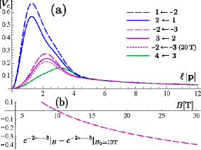
Figure 3: (a) Momentum profiles of the many-body corrections $\triangle\epsilon^{b\leftarrow a}/\eta^{b\leftarrow a}$ for some typical channels, with $v=1.1\times 10^{6}$m/s, $\gamma_{1}=404\,{\rm meV}$, $\triangle=18\,{\rm meV}$ and $v_{4}/v=-0.04$ at $B$= 10 T. (b) $c^{-2\leftarrow-3}|_{B}-c^{-2\leftarrow-3}|_{B_{0}}$ reveals the running of $v^{\rm ren}|_{B}$.

Figure 3 (a) shows for some typical resonance channels the (rescaled) momentum profiles $\gamma_{\bf p}^{2}\,[\cdots]$ in $\triangle\epsilon^{b\leftarrow a}$ of Eq. (III), which, when integrated over $\ell|{\bf p}|$, give $\triangle\epsilon^{b\leftarrow a}/\eta^{b\leftarrow a}$ in units of $V_{c}$. Note that the slowly decreasing high-momentum tail $\sim(\sqrt{2}/4)/(\ell\,|{\bf p}|)$, common to all profiles, is responsible for the UV divergence. This numerically verifies the UV scaling law (31) of the ratios $\triangle\epsilon^{b\leftarrow a}/\eta^{b\leftarrow a}$.

For renormalization let us refer to a specific channel $(b_{0}\leftarrow a_{0})$ and choose to define $v^{\rm ren}$ and other renormalized parameters by writing $\epsilon_{\rm exc}^{b_{0}\leftarrow a_{0}}=\omega_{c}^{\rm ren}\,(\eta_{b_{0}}-\eta_{a_{0}})$ at magnetic field $B$, or equivalently, $(\triangle\epsilon^{b_{0}a_{0}})^{\rm ren}=0$, which yields $\delta v=-(\alpha/\sqrt{2}\,\epsilon_{b})\,c^{b_{0}\leftarrow a_{0}}$. The renormalized velocity then runs with $B$,

$$v^{\rm ren}|_{B}=v^{\rm ren}|_{B_{0}}+{\alpha\over{\sqrt{2}\,\epsilon_{b}}}\,\Big{\{}c^{b_{0}\leftarrow a_{0}}|_{B}-c^{b_{0}\leftarrow a_{0}}|_{B_{0}}\Big{\}},$$ (32)

and decreases gradually with increasing $B$. The leading correction $c^{b_{0}\leftarrow a_{0}}|_{B}-c^{b_{0}\leftarrow a_{0}}|_{B_{0}}\sim-(\sqrt{2}/8)\,\log(B/B_{0})$ is logarithmic but corrections coming from finite terms $F^{b_{0}a_{0}}$ are equally important for relatively low magnetic fields. For definiteness let us take $L_{-2}\leftarrow L_{-3}$ as the reference channel, as chosen experimentally. HJTS For this channel the contribution from the low-momentum region decreases with $B$, as seen from the $(-2\leftarrow-3)$ profiles for $B=(10{\rm T},20{\rm T})$ in Fig. 3 (a), and numerically the correction is roughly doubled, fncba

$$c^{-2\leftarrow-3}|_{B}-c^{-2\leftarrow-3}|_{B_{0}}\approx-2.1\times{\sqrt{2}\over{8}}\,\log{B\over{B_{0}}}$$ (33)

over the range $10\,{\rm T}\lesssim B\lesssim 30\,{\rm T}$, as shown in Fig. 3 (b). One can multiply it by factor $\alpha/(\sqrt{2}\,\epsilon_{b}v)\sim 1.5/\epsilon_{b}\sim 0.3$ (with $\epsilon_{b}\sim 5$) to estimate the rate of decrease in $v^{\rm ren}|_{B}$ with $B$, which is about 10% for $B=10{\rm T}\rightarrow 20{\rm T}$.

The renormalized Coulombic corrections in all other channels are thereby fixed uniquely,

$$(\triangle\epsilon^{ba})^{\rm ren}=V_{c}\,\eta^{b\leftarrow a}\,(c^{b\leftarrow a}-c^{b_{0}\leftarrow a_{0}})|_{B}.$$ (34)

These observable corrections are essentially calculated from the profiles in the low-momentum region $\ell\,|{\bf p}|\lesssim 15$.

It is enlightening to write the resonance energies as

$$\epsilon_{\rm exc}^{b\leftarrow a} = (\eta_{b}-\eta_{a})\,\Big{[}\omega_{c}^{\rm ren}+V_{c}\,\tilde{\triangle}\,c^{b,a}\Big{]},$$ (35)

$$\tilde{\triangle}c^{b,a} \equiv {\eta^{b\leftarrow a}\over{\eta_{b}-\eta_{a}}}\,(c^{b\leftarrow a}-c^{b_{0}\leftarrow a_{0}})|_{B},$$ (36)

so that the Coulombic corrections $V_{c}\,\tilde{\triangle}\,c^{b,a}$ seemingly arise relative to $\omega_{c}^{\rm ren}$. Using the set of parameters in Eq. (7), one finds, for some typical intraband channels,

$$\tilde{\triangle}c^{5,4} \stackrel{{\scriptstyle\nu=16}}{{=}} -0.317,\ \ (-0.259),$$

$$\tilde{\triangle}c^{4,3} \stackrel{{\scriptstyle\nu=12}}{{=}} -0.223,\ \ (-0.175),$$

$$\tilde{\triangle}c^{3,2} \stackrel{{\scriptstyle\nu=8}}{{=}} -0.073,\ \ (-0.040),$$

$$\tilde{\triangle}c^{2,1} \stackrel{{\scriptstyle\nu=4}}{{=}} 0.650,\ \ (0.533),$$

$$\tilde{\triangle}c^{1,-2} \stackrel{{\scriptstyle\nu=-4}}{{=}} 0.897,\ \ (0.675),$$

$$\tilde{\triangle}c^{-2,-3} \stackrel{{\scriptstyle\nu=-8}}{{=}} 0,\ \ (0),$$

$$\tilde{\triangle}c^{-3,-4} \stackrel{{\scriptstyle\nu=-12}}{{=}} -0.165,\ \ (-0.150),$$

$$\tilde{\triangle}c^{-4,-5} \stackrel{{\scriptstyle\nu=-16}}{{=}} -0.275,\ \ (-0.247),$$ (37)

at $B=10$T ($B=20$T). For comparison, setting $v_{4}=\triangle=0$ yields the electron-hole symmetric values $\tilde{\triangle}c^{1,-2}=0.815$, $\tilde{\triangle}c^{-2,-3}=0$, $\tilde{\triangle}c^{-3,-4}=-0.159$ and $\tilde{\triangle}c^{-5,-4}=-0.303$ at $B=10$T. Similarly, some interband channels yield

$$\tilde{\triangle}c^{3,-2} \stackrel{{\scriptstyle\nu=-4}}{{=}} 0.353,\ \ (0.375),$$

$$\tilde{\triangle}c^{2,-3} \stackrel{{\scriptstyle\nu=-8}}{{=}} 0.370,\ \ (0.363),$$

$$\tilde{\triangle}c^{3,-4} \stackrel{{\scriptstyle\nu=-12}}{{=}} 0.261,\ \ (0.278).$$ (38)

Note that those corrections are ordered regularly in magnitude for a sequence of resonances; see also the theoretical curves for $\epsilon_{\rm exc}^{b\leftarrow a}$ in Figs. 4(b) and 4(d).

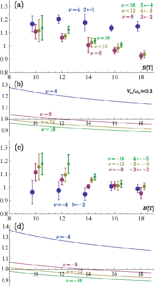
Figure 4: Cyclotron-resonance data of Ref. HJTS, with error bars, reorganized in the form $\epsilon^{b\leftarrow a}_{\rm exc}/(\eta^{b}-\eta^{a})$ and plotted in units of $\omega_{c}=\sqrt{2}\,v_{0}/\ell$ (with $v_{0}=1.1\times 10^{6}$m/s) for $\gamma_{1}\approx 404\,{\rm meV}$, $\triangle\approx 18\,{\rm meV}$ and $v_{4}/v\equiv-\gamma_{4}/\gamma_{0}\approx-0.04$. (a) Electron data; for clarity the data points, originally at $B$=(10, 12, 14, 16, 18) T, are slightly shifted in $B$. (b) Theoretical expectation according to Eq. (̃32), with $V_{c}/\omega_{c}\approx 0.3$ (or $\epsilon_{b}\approx 5)$. (c) Hole data. (d) Theoretical curves.

Our formula (35) summarizes the effect of renormalization in a concise form and is also useful in analyzing the experimental results. One may rescale the observed excitation energies $\epsilon^{b\leftarrow a}_{\rm exc}$ in the form $\epsilon^{b\leftarrow a}_{\rm exc}/(\eta_{b}-\eta_{a})$ and plot them in units of $1/\ell\propto\sqrt{B}$ for each given value of $B$. The Coulombic many-body effect will then be seen as a variation in characteristic velocity $v^{\rm ren}|_{B}[1+O(V_{c})]$ from one resonance to another, and a deviation of $\omega_{c}^{\rm ren}$ from $\sqrt{B}$ behavior would indicate the running of $v^{\rm ren}$ with $B$.

Figures 4(a) and 4(c) show such plots for the series of cyclotron resonance reported in Ref. HJTS, . Both electron and hole data are plotted in units of $\omega_{c}=\sqrt{2}\,v_{0}/\ell\approx 40\sqrt{B[{\rm T}]}$ meV (with reference velocity $v_{0}=1.1\times 10^{6}$ m/s kept fixed). These plots offer a closer look into the plots in Fig. 2.

They are to be compared with Figs. 4(b) and 4(d), which illustrate how each resonance would behave with $B$, according to Eq. (35), for $V_{c}\approx 11\sqrt{B[{\rm T}]}$ meV (or $\epsilon_{b}\approx 5)$. The $\nu=-8$ curve for $\epsilon_{\rm exc}^{-2\leftarrow-3}|_{\nu=-8}$, in particular, represents the running of $v^{\rm ren}|_{B}$ according to Eq. (32) (normalized to 1 at $B_{0}=14$T). These theoretical curves and experimental data look similar but differ in details. They are not quite consistent, but there are some notable features: (i) The $2\leftarrow 1$ and $1\leftarrow-2$ resonances (the $\nu=\pm 4$ data) appear distinct from the rest, especially in their variation with $B$. In addition, the $\nu=\pm 4$ theoretical curves are separated from the rest by appreciable Coulombic gaps, but such a gap is not seen in the hole data. This would indicate, as noted in Sec. II, that the $n=(0,1)$ sector in bilayer graphene is significantly modified from the naive one we have supposed.

(ii) The $\nu=(8,12,16)$ electron data and the $\nu=(-8,-12,-16)$ hole data show a general trend to decrease with $B$, consistent with possible running of $v^{\rm ren}$ with $B$. Such ($\sim$ logarithmic) running of $v^{\rm ren}|_{B}$ is a direct consequence of renormalization and is thus the key signature of the Coulomb interaction. In both electron and hole data $v^{\rm ren}$ appears to run in the same way at a rate somewhat faster than naively expected. Such enhanced running could in part be attributed to possible quantum screening KSpzm of the Coulomb interaction in graphene such that $\epsilon_{b}$ is effectively larger KSbgr for lower $B$.

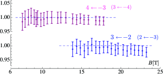
Figure 5: Interband cyclotron resonances in bilayer inclusions in multilayer epitaxial graphene reported by Orlita et al. Here some data from Ref. OFB, are analyzed in the same way as in Fig. 4, using $v_{0}=1.02\times 10^{6}$m/s and $\gamma_{1}\approx 385\,{\rm meV}$ for zero asymmetry $\triangle=\gamma_{4}=0$.

Interband cyclotron resonance was recently observed by Orlita et al. OFB in bilayer inclusions in multilayer epitaxial graphene on the C-face of SiC. They identify some $n-1\leftarrow-n$ [or $n\leftarrow-(n-1)$] resonances with $n\geq 3$ and obtain, via fitting, $v\approx 1.02\times 10^{6}$ m/s and $\gamma_{1}\approx 385$ meV, which are somewhat smaller than those for bilayer graphene.

Some of their data are analyzed according to our formula (35) in Fig. 5; there we have set $\gamma_{4}=\triangle=0$ since this experiment searched for no intraband resonances which would clarify a possible electron-hole asymmetry. The data appear to indicate slight running of $v^{\rm ren}$ with $B$, far slower than in the data in Fig. 4 on bilayer graphene. This suggests that the Coulomb interaction could be significantly weaker (or more efficiently screened) in multilayered epitaxial graphene than in exfoliated bilayer graphene.

IV summary and discussion

Experiment suggests that bilayer graphene has intrinsic electron-hole asymmetry due to subleading intralayer and interlayer couplings. In this paper we have studied cyclotron resonance in bilayer graphene with such asymmetry taken into account.

The set of asymmetry parameters, $\triangle\approx 18$ meV and $\gamma_{4}/\gamma_{0}\approx 0.04$ derived from independent measurements, entails a considerable modification of Landau levels in bilayer graphene and improves the theoretical fit to the data on cyclotron resonance between higher levels $|n|\geq 2$ in both electron and hole bands. In contrast, the fit to the data on $(2\leftarrow 1)$ and $(1\leftarrow-2)$ resonances appears somewhat puzzling, and this suggests that the zero- and pseudo-zero-mode Landau levels $n=(0,\pm 1)$ are further affected by some sources other than $\triangle$ and $\gamma_{4}$. It would be important to clarify, both theoretically and experimentally, the detailed structure of this special sector in bilayer graphene.

The Coulombic many-body corrections to cyclotron resonance in graphene, unlike in standard quantum-Hall systems, are afflicted with UV divergences, and one has to carry out renormalization to extract genuine observable corrections. We have shown how to perform renormalization for bilayer graphene under a magnetic field by first constructing necessary conterterms in free space. This renormalization program, formulated analytically, can equally be handled numerically in practical calculations by use of the reduced matrix Hamiltonian $\hat{\cal H}_{\rm red}^{\rm ren}$ in Eq. (10) and counterterm $\delta_{\rm ct}\hat{\cal H}_{\rm red}^{\rm ren}$ in Eq. (26). As a further illustration, we present the renormalization program for monolayer graphene with a possible valley gap in Appendix B.

Equation (35) summarizes the effect of renormalization on cyclotron-resonance energies in a neat and concise form. This formula is also useful in analyzing the experimental data; it magnifies possible effects of the Coulombic corrections per channel and running of the renormalized velocity $v^{\rm ren}$ with $B$, as we have seen in Sec. III. In particular, the nearly logarithmic running of $v^{\rm ren}$ is a direct consequence of renormalization, specific to graphene. EGM ; AddRef It is remarkable that such a renormalization effect is apparently seen in the data.

More detailed measurements of cyclotron resonance, both intraband and interband ones, are highly desired to pin down the many-body effects as well as the structure of the zero-mode and pseudo-zero-mode sector in bilayer graphene.

Appendix A Analysis of divergence

In this appendix we examine the UV structure of the Coulomb exchange correction. Let us first look at ${\cal H}_{+}$ in Eq. (5) and construct the electron propagator in free space,

$$\langle\Psi(x)\Psi^{{\dagger}}(x^{\prime})\rangle=\langle x|i/(i\partial_{t}-{\cal H}_{+})|x^{\prime}\rangle$$ (39)

with $|x\rangle\equiv|{\bf x}\rangle\,|t\rangle$. We divide ${\cal H}_{+}$ into $2\times 2$ blocks,

$${\cal H}_{+} = \left(\begin{array}[]{cc}m\,\sigma_{3}&v\,P+v_{4}\,Q\\ v\,P+v_{4}\,Q^{{\dagger}}&-m\,\sigma_{3}+\triangle+\gamma_{1}\,\sigma_{1}\\ \end{array}\right),$$ (42)

where we have set $m\equiv u/2$; $P=p^{{\dagger}}\sigma_{+}+p\,\sigma_{-}$ with $p=p_{x}+i\,p_{y}$ and $\sigma_{\pm}=(\sigma_{1}\pm i\sigma_{2})/2$; $Q={\rm diag.}(p^{{\dagger}},p)$; the unit matrix $1$, which, e.g., multiplies $\triangle$ in Eq.$~{}(\ref{HplusAp})$, will be suppressed in what follows.

We go to the Fourier $({\bf p},\omega)$ space and invert $(\omega-{\cal H}_{+})$ in this $2\times 2$ block form. A direct calculation yields $\langle\Psi\Psi^{{\dagger}}\rangle_{jk}=i\,N_{jk}/D$ with

$$N_{11} = \Gamma+\{(v^{2}+v_{4}^{2})\,\gamma_{1}+2v_{4}v\,(\omega-\triangle)\}\,P\sigma_{1}P$$

$$+m\,(\Xi-2\,\triangle\,\omega+\triangle^{2}-\gamma_{1}^{2})\,\sigma_{3},$$

$$N_{22} = \Gamma-2\,v\,(v\,\triangle-v_{4}\gamma_{1})\,{\bf p}^{2}$$

$$+\omega\,(\gamma_{1}^{2}-\triangle^{2})+\triangle\,(\Xi+2m^{2})$$

$$-m\,\Xi\,\sigma_{3}+\{\gamma_{1}\,(\omega^{2}-m^{2})+2\,v_{4}v\,{\bf p}^{2}\,\omega\}\,\sigma_{1},$$

$$N_{12} = v\,(\omega^{2}-v_{+}v_{-}\,{\bf p}^{2}+m^{2})\,P$$ (43)

$$+2m\,v_{4}\,\sigma_{3}P+v_{4}\,\Xi\,Q$$

$$+(v_{4}\,\gamma_{1}-v\,\triangle)\,(\omega+m\,\sigma_{3})\,P$$

$$+(v\,\gamma_{1}-v_{4}\triangle)\,(\omega+m\,\sigma_{3})\,Q,$$

and $N_{21}=(N_{12})^{{\dagger}}$, where

$$\Gamma = \omega\,\{(\omega-\triangle)^{2}-(v^{2}+v_{4}^{2})\,{\bf p}^{2}-m^{2}-\gamma_{1}^{2}\}$$

$$+\{(v^{2}+v_{4}^{2})\,\triangle-2\,v_{4}v\,\gamma_{1}\}\,{\bf p}^{2},$$

$$\Xi = \omega^{2}+v_{+}v_{-}\,{\bf p}^{2}-m^{2};$$ (44)

$v_{\pm}\equiv v\pm v_{4}$ and $P\sigma_{1}P=(p^{{\dagger}})^{2}\,\sigma_{+}+p^{2}\,\sigma_{-}$. The denominator $D={\rm det}\,(\omega-{\cal H}_{+})$ is cast in the form

$$D = \{\omega^{2}-\triangle\,\omega-(v^{2}+v_{4}^{2})\,{\bf p}^{2}-m^{2}\}^{2}$$ (45)

$$-(\gamma_{1}\,\omega+2v_{4}v\,{\bf p}^{2})^{2}$$

$$-m^{2}\,(4\,v^{2}{\bf p}^{2}-\gamma_{1}^{2}-\triangle^{2}),$$

which, for $u=2m\rightarrow 0$, leads to the band spectra $\{\epsilon_{i}\}$ in Eq. (8).

The Coulomb exchange correction to $O(\alpha/\ell)$ is written as the convolution $\sum_{\bf k}v_{\bf k}\,iS({\bf p+k})$ of $v_{\bf k}=2\pi\alpha/|{\bf k}|$ and the instantaneous limit of the electron propagator $\langle\Psi\,\Psi^{{\dagger}}\rangle|_{t^{\prime}=t}=\int(d\omega/2\pi)\,\langle\Psi\,\Psi^{{\dagger}}\rangle_{\omega,{\bf p}}=iS({\bf p})$. In particular, divergences arise from the portion of $S({\bf p})$, that decreases like $1/|{\bf p}|$ or slower for ${\bf p}\rightarrow\infty$, and we shall focus on that portion.

Integration over $\omega$, with the standard boundary condition, is readily carried out, yielding, e.g.,

$$\int{d\omega\over{2\pi}}{1\over{D(\omega)}}=i\,{a+b+c+d\over{(a+c)(b+c)(a+d)(b+d)}},$$ (46)

where $D(\omega)=(\omega-a)(\omega-b)(\omega+c)(\omega+d)$ $(a,b,c,d>0)$ is short for $D$ in Eq. (45). When the integrand is $\omega/D$, replace the numerator on the the right-hand side with $ab-cd$; for $\omega^{2}/D$ replace it with $-ab(c+d)-(a+b)cd$. Actually, this structure combined with the band spectra (8) gives rise to a simple rule to handle the integration over $\omega$: One can effectively replace

$$\omega \rightarrow (\triangle-r\,\gamma_{1})/2+\cdots,$$

$$\omega^{2} \rightarrow -v_{+}v_{-}\,{\bf p}^{2}+\cdots,$$ (47)

in $N_{jk}$ in evaluating their large-${\bf p}$ behavior.

One may further note the following: (i) The denominator $(a+c)...(b+d)\approx 16v^{2}v_{+}v_{-}\,({\bf p}^{2})^{2}$ for large ${\bf p}$. (ii) For $v_{4}\rightarrow 0$ and $\triangle\rightarrow 0$, $D(\omega)$ becomes an even function of $\omega$. As a result, odd powers of $\omega$ in $N_{jk}$ necessarily lead to $v_{4}\gamma_{1}$ or $\triangle$, and are one power of $|{\bf p}|$ less than naively expected; e.g., $ab-cd\approx 2(v\triangle-v_{4}\,\gamma_{1})\,|{\bf p}|$; corrections of the form $v_{4}\,m$ do not arise since $D$ is even in $m=u/2$.

With this in mind one can now retain only the portion

$$N_{11} \approx \Gamma+\{(v^{2}+v_{4}^{2})\,\gamma_{1}+2v_{4}v\,(\omega-\triangle)\}\,P\sigma_{1}P,$$

$$N_{22} \approx \Gamma-2\,v\,(v\,\triangle-v_{4}\gamma_{1})\,{\bf p}^{2}+(\gamma_{1}\,\omega^{2}+2\,v_{4}v\,{\bf p}^{2}\,\omega)\,\sigma_{1},$$

$$N_{12} \approx v\,(\omega^{2}-v_{+}v_{-}\,{\bf p}^{2})\,P,$$ (48)

for further consideration. Note that, in view of Eq. (47), the particular combination $\Xi$, despite its appearance, yields no divergent correction. As a result, terms $\propto\sigma_{3}$ in $N_{11}$ and $N_{22}$ lead to finite corrections. This fact has the important consequence that the interlayer bias $u=2m$ requires no infinite renormalization.

The structure of the $O(\alpha/\ell)$ Coulombic selfenergy correction precisely reflects the structure of $S({\bf p})$ after convolution with $v_{\bf p}\propto 1/|{\bf p}|$. Let us therefore compare Eq. (48) with ${\cal H}_{+}$ in Eq. (42). Applying first the rule (47) to $N_{12}$ in Eq. (48) yields the asymptotic form

$$\langle\Psi\Psi^{{\dagger}}\rangle_{12}|_{t=t^{\prime}}=P/(2\,|{\bf p}|)+\cdots.$$ (49)

This $P/2\,|{\bf p}|$ term leads to a divergent correction of the form $\propto P\,\log\Lambda^{2}$, which requires renormalization of velocity velrenorm $v$. Actually this leading form $P/2\,|{\bf p}|$ is the same as the one obtained previously KScr for $v_{4}=\triangle=0$, and this implies that (the divergent part of) velocity renormalization is unaffected by the electron-hole asymmetry $\propto v_{4},\triangle$. On the other hand, the portion $\propto Q$ in $\langle\Psi\Psi^{{\dagger}}\rangle_{12}$ has the asymptotic form $\propto Q/{\bf p}^{2}$ which leads to no divergence and this means that $v_{4}$ remains finite.

Let us next consider $\langle\Psi\Psi^{{\dagger}}\rangle_{11}$ or $N_{11}$ in Eq. (48). Its $P\sigma_{1}P$ portion has the asymptotic structure $P\sigma_{1}P/|{\bf p}|^{3}$, which, though potentially singular, actually yields no divergent correction via symmetric ${\bf p}$ integration [since $P\sigma_{1}P\propto p^{2}$ or $(p^{{\dagger}})^{2}$]. The remaining portion $\propto\Gamma$ is common to $N_{11}$ and $N_{22}$. Those common $\Gamma$ terms, though leading to a divergent correction, simply shift the zero of energy and are of no physical relevance. One can now eliminate this $\Gamma$ term from $\langle\Psi\Psi^{{\dagger}}\rangle_{22}|_{t=t^{\prime}}$ and determine its asymptotic form

$$\langle\Psi\Psi^{{\dagger}}\rangle_{22}|_{t=t^{\prime}}={v\,\gamma_{1}-v_{4}\,\triangle\over{4\,v_{+}v_{-}|{\bf p}|}}\,\sigma_{1}+{v\,\triangle-v_{4}\,\gamma_{1}\over{2\,v_{+}v_{-}|{\bf p}|}}+\cdots.$$ (50)

This implies that both $\gamma_{1}$ and $\triangle$ undergo infinite renormalization. Evaluating the convolution integral $\int d^{2}{\bf k}\,v_{\bf k}\,S({\bf p+k})$ with momentum cutoff $\Lambda$ eventually leads to the counterterms in Eqs. (22) $\sim$ (24).

Appendix B monolayer graphene with a valley gap

In this appendix we outline the renormalization prescription for monolayer graphene with a possible valley gap $M$. The effective Hamiltonian is written as

$${\cal H}_{+}=v\,{\bf p}\cdot\vec{\sigma}+M\,\sigma_{3}$$ (51)

at one valley and acts on a two-component spinor of the form $\Psi=(\psi_{A},\psi_{B})^{\rm t}$. One can pass to another valley by setting $M\rightarrow-M$ and $\Psi\rightarrow\Psi^{\prime}=(-\psi^{\prime}_{B},\psi^{\prime}_{A})^{\rm t}$.

Using the instantaneous propagator

$$\langle\Psi\Psi^{{\dagger}}\rangle_{t=t^{\prime}}={1\over{2}}\,{v\,{\bf p}\cdot\vec{\sigma}+M\,\sigma_{3}\over{\sqrt{v^{2}\,{\bf p}^{2}+M^{2}}}}$$ (52)

one can calculate the Coulombic selfenergy correction to $O(\alpha)$ and find divergences of the form

$$\delta v\sim-(\alpha/8\epsilon_{b})\,\log\Lambda^{2},\ \delta M=2\,(M^{\rm ren}/v^{\rm ren})\,\delta v,$$ (53)

which implies that the mass gap $M$, as well as $v$, undergoes renormalization.

Let us now pass to the $B\not=0$ case and denote the zeroth order Landau-level spectrum as $\epsilon_{n}^{\rm ren}=\omega_{c}^{\rm ren}\,\eta_{n}$ with $\omega_{c}^{\rm ren}=\sqrt{2}\,v^{\rm ren}/\ell$ and

$$\eta_{n}={\rm sgn}[n]\,\sqrt{|n|+(M^{\rm ren}/\omega_{c}^{\rm ren})^{2}}.$$ (54)

Letting $\delta_{\rm ct}=\delta v\,\partial/\partial v^{\rm ren}+\delta M\,\partial/\partial M^{\rm ren}$ act on $\epsilon_{n}^{\rm ren}$ then yields the counterterm $\delta_{\rm ct}\epsilon_{n}^{\rm ren}$. In particular, one finds that ${\cal D}\eta_{n}$ in Eq. (29) is now replaced by

$${\cal D}\eta_{n}\rightarrow(M^{\rm ren}/\omega_{c}^{\rm ren})^{2}/\eta_{n}.$$ (55)

With Eqs. (54) and (55), velocity and mass renormalization for monolayer graphene in a magnetic field is carried out according to formula (35); we have checked numerically that this renormalization program works correctly.

References

- (1) K. S. Novoselov, A. K. Geim, S. V. Morozov, D. Jiang, M. I. Katsnelson, I. V. Grigorieva, S. V. Dubonos, and A. A. Firsov, Nature (London) 438, 197 (2005).
- (2) Y. Zhang, Y.-W. Tan, H. L. Stormer, and P. Kim, Nature (London) 438, 201 (2005).
- (3) Y. Zhang, Z. Jiang, J.P. Small, M.S. Purewal, Y.-W. Tan, M. Fazlollahi, J.D. Chudow, J.A. Jaszczak, H. L. Stormer, and P. Kim, Phys. Rev. Lett. 96, 136806 (2006).
- (4) N. H. Shon and T. Ando, J. Phys. Soc. Jpn. 67, 2421 (1998); Y. Zheng and T. Ando, Phys. Rev. B 65, 245420 (2002).
- (5) N. M. R. Peres, F. Guinea, and A. H. Castro Neto, Phys. Rev. B 73, 125411 (2006).
- (6) W. Kohn, Phys. Rev. 123, 1242 (1961).
- (7) For many-body corrections in quantum Hall systems, see K. Asano and T. Ando, Phys. Rev. B 58, 1485 (1998). Kohn’s theorem is also discussed for graphene by R. Roldán, J.-N, Fuchs, and M. O. Goerbig, Phys. Rev. B 82, 205418 (2010).
- (8) D. S. L. Abergel and V. I. Fal’ko, Phys. Rev. B 75, 155430 (2007).
- (9) A. Iyengar, J. Wang, H. A. Fertig, and L. Brey, Phys. Rev. B 75, 125430 (2007).
- (10) Yu. A. Bychkov and G. Martinez, Phys. Rev. B 77, 125417 (2008).
- (11) S. Viola Kusminskiy, D. K. Campbell, and A. H. Castro Neto, Euro. Phys. Lett. 85, 58005 (2009).
- (12) K. Shizuya, Phys. Rev. B 81, 075407 (2010).
- (13) K. S. Novoselov, E. McCann, S. V. Morozov, V. I. Fal’ko, M. I. Katsnelson, U. Zeitler, D. Jiang, F. Schedin, and A. K. Geim, Nat. Phys. 2, 177 (2006).
- (14) E. McCann and V. I. Fal’ko, Phys. Rev. Lett. 96, 086805 (2006).
- (15) T. Ohta, A. Bostwick, T. Seyller, K. Horn, and E. Rotenberg, Science 313, 951 (2006).
- (16) E. McCann, Phys. Rev. B 74, 161403(R) (2006).
- (17) E. V. Castro, K. S. Novoselov, S. V. Morozov, N. M. R. Peres, J. M. B. Lopes dos Santos, J. Nilsson, F. Guinea, A. K. Geim, and A. H. Castro Neto, Phys. Rev. Lett. 99, 216802 (2007).
- (18) J. B. Oostinga, H. B. Heersche, X. Liu, A. F. Morpurgo, and L. M. K. Vandersypen, Nature Mater. 7, 151 (2008).
- (19) M. Mucha-Kruczyński, E. McCann, and V. I. Fal’ko, Solid State Commun. 149, 1111 (2009).
- (20) Z. Jiang, E. A. Henriksen, L. C. Tung, Y.-J. Wang, M. E. Schwartz, M. Y. Han, P. Kim, and H. L. Stormer, Phys. Rev. Lett. 98, 197403 (2007).
- (21) R. S. Deacon, K.-C. Chuang, R. J. Nicholas, K. S. Novoselov, and A. K. Geim, Phys. Rev. B 76, 081406(R) (2007).
- (22) E. A. Henriksen, P. Cadden-Zimansky, Z. Jiang, Z. Q. Li, L.-C. Tung, M. E. Schwartz, M. Takita, Y.-J. Wang, P. Kim, and H. L. Stormer, Phys. Rev. Lett. 104, 067404 (2010).
- (23) E. A. Henriksen, Z. Jiang, L.-C. Tung, M. E. Schwartz, M. Takita, Y.-J. Wang, P. Kim, and H. L. Stormer, Phys. Rev. Lett. 100, 087403 (2008).
- (24) M. Orlita, C. Faugeras, J. Borysiuk, J. M. Baranowski, W. Strupiński, M. Sprinkle, C. Berger, W. A. de Heer, D. M. Basko, G. Martinez, and M. Potemski, Phys. Rev. B 83, 125302 (2011).
- (25) L. M. Malard, J. Nilsson, D. C. Elias, J. C. Brant, F. Plentz, E. S. Alves, A. H. Castro Neto, and M. A. Pimenta, Phys. Rev. B 76, 201401(R) (2007).
- (26) L. M. Zhang, Z. Q. Li, D. N. Basov, and M. M. Fogler, Z. Hao, and M. C. Martin, Phys. Rev. B 78, 235408 (2008).
- (27) Z. Q. Li, E. A. Henriksen, Z. Jiang, Z. Hao, M. C. Martin, P. Kim, H. L. Stormer, and D. N. Basov, Phys. Rev. Lett. 102, 037403 (2009).
- (28) A. B. Kuzmenko, E. van Heumen, D. van der Marel, P. Lerch, P. Blake, K. S. Novoselov, and A. K. Geim, Phys. Rev. B 79, 115441 (2009).
- (29) J. Nilsson, A. H. Castro Neto, F. Guinea, and N. M. R. Peres, Phys. Rev. B 78, 045405 (2008).
- (30) D. S. L. Abergel and T. Chakraborty, Phys. Rev. Lett. 102, 056807 (2009).
- (31) T. Misumi and K. Shizuya, Phys. Rev. B 77, 195423 (2008); K. Shizuya, Phys. Rev. B 75, 245417 (2007).
- (32) Numerically, for meV crossing takes place at T.
- (33) Y. Barlas, R. Côté, K. Nomura, and A. H. MacDonald, Phys. Rev. Lett. 101, 097601 (2008).
- (34) K. Shizuya, Phys. Rev. B 79, 165402 (2009).
- (35) R. Côté, J. Lambert, Y. Barlas, and A. H. MacDonald, Phys. Rev. B 82, 035445 (2010).
- (36) S. M. Girvin, A. H. MacDonald, and P. M. Platzman, Phys. Rev. B 33, 2481 (1986).
- (37) J. González, F. Guinea, and M. A. H. Vozmediano, Nucl. Phys. B 424, 595 (1994).
- (38) For an eigenmode of with eigenvalue one generally finds that for an arbitrary variation .
- (39) is calculated by integrating the underlying momentum profile over the interval , with the momentum cutoff kept fixed.
- (40) Recently the effect of renormalization on the electronic spectrum has been measured for suspended graphene, in which runs with the electron density as . See, D. C. Elias, R. V. Gorbachev, A. S. Mayorov, S. V. Morozov, A. A. Zhukov, P. Blake, K. S. Novoselov, A. K. Geim, and F. Guinea, preprint arXiv:1104.1396.
- (41) Renormalization of electron interactions in bilayer graphene under zero magnetic field was discussed by Y. Barlas and K. Yang, Phys. Rev. B 80, 161408(R) (2009); O. Vafek and K. Yang, Phys. Rev. B 81, 041401(R) (2010); R. Nandkishore and L. Levitov, Phys. Rev. B 82, 115431 (2010).