Electromagnetic Decay of the $\Sigma^{0}(1385)$ to $\Lambda\gamma$

Abstract

The electromagnetic decay $\Sigma^{0}(1385)\to\Lambda\gamma$ was studied using the CLAS detector at the Thomas Jefferson National Accelerator Facility. A real photon beam with a maximum energy of 3.8 GeV was incident on a proton target, producing an exclusive final state of $K^{+}\Sigma^{*0}$. We report the decay widths ratio $\Sigma^{0}(1385)\to\Lambda\gamma$/ $\Sigma^{0}(1385)\to\Lambda\pi^{0}$ = $1.42\pm 0.12(\text{stat})_{-0.07}^{+0.11}(\text{sys})$%. This ratio is larger than most theoretical predictions by factors ranging from 1.5-3, but is consistent with the only other experimental measurement. From the reported ratio we calculate the partial width and electromagnetic transition magnetic moment for $\Sigma^{0}(1385)\to\Lambda\gamma$.

I Introduction

One well-known success of the constituent quark model (CQM) is its prediction of the low-mass baryon magnetic moments, using just the SU(6) wavefunctions Beg ; Rubin . Calculations of the magnetic moments IsgKar , assuming that quarks behave as point-like Dirac dipoles, are typically within $\sim$10% of the current measured values PDG . However, today we know that the spin of the proton is much more complex than the CQM representation, with only about one-third of the proton’s spin coming from the quarks and the rest of the spin resulting from a combination of the gluon spins and the orbital angular momentum of the quarks Alexakhin ; Airapetian . Clearly, the CQM is an over-simplification of the spin dynamics inside baryons, yet somehow the CQM captures the degrees of freedom that are relevant to the measured magnetic moments. Further measurements of baryon magnetic moments, utilizing the electromagnetic decays of excited baryons, will continue to test our understanding of baryon wavefunctions.

Experimentally, it is difficult to measure the electromagnetic (EM) transitions of decuplet-to-octet baryons because of the competition between EM and strong decays. For example, the branching ratio for EM decay of the $\Delta$ resonance has been measured to be about 0.55% PDG and branching ratios for other decuplet baryons are predicted to be of the same order of magnitude. The EM transition form factors for the $\Delta$ may be directly measured via pion photoproduction Dalitz ; Sato .

It has been shown Lee that pion cloud effects contribute significantly ($\sim$40%) to the $\gamma p\to\Delta^{+}$ magnetic dipole transition form factor, $G_{M}(Q^{2})$, at low $Q^{2}$ (below $\sim 0.1$ GeV²). In the naive non-relativistic quark model CQM , the value of $G_{M}(0)$ is directly proportional to the proton magnetic moment, and measurements of $G_{M}$ near $Q^{2}=0$ can only be explained (within this quark model) if the experimental magnetic moment is lowered by about 30%. This again suggests that the CQM is an over-simplification of reality.

To extend these measurements to the other decuplet baryons, which have non-zero strangeness, hyperons must be produced through strangeness-conserving reactions. Then their EM decay, which has a small branching ratio, must be measured directly. Although these measurements are difficult, it is important to measure the EM decays of strange baryons to extract information on their wavefunctions, which in turn, constrains theoretical models of baryon structure. The measurements of EM transition form factors for decuplet baryons with strangeness may also be sensitive to meson cloud effects. A comparison of the EM decay measurements to predictions of quark models for decay of decuplet hyperons, $\Sigma^{*}$, to octet hyperons, $Y$, can provide a measure of the importance of meson cloud diagrams in the $\Sigma^{*}\to Y\gamma$ transition.

Here, we present measurements of the EM decay $\Sigma^{*0}\to\Lambda\gamma$ normalized to the strong decay $\Sigma^{*0}\to\Lambda\pi^{0}$. The present results can be compared to previous measurements of the $\Sigma^{*0}$ EM decay Taylor (also from CLAS data) that had a larger uncertainty ($\sim$25% statistical and $\sim$15% systematic uncertainty). The smaller uncertainties here are due to a larger data set (more than 10 times bigger) and, subsequently, better control over systematic uncertainties. The reduced uncertainty is important because, as mentioned above, meson cloud effects are predicted to be on the order of $\sim$30-40%. In order to quantify the effect of meson clouds for baryons with non-zero strangeness, it is desirable to keep measurement uncertainties below $\sim$10%.

Table 1: Theoretical predictions for the models referenced in the text and the experimental values for the electromagnetic decay widths (in keV).

Model	$\Delta(1232)\to N\gamma$	$\Sigma(1193)\to\Lambda\gamma$	$\Sigma(1385)\to\Lambda\gamma$
NRQM Koniuk ; kaxiras ; DHK	360	8.6	273
RCQM warns		4.1	267
$\chi$CQM wagner	350		265
MIT Bag kaxiras		4.6	152
Soliton Schat			243
Skyrme Abada ; Haberichter	309-326		157-209
Algebraic model Bijker	341.5	8.6	221.3
HB$\chi$PT butler †	(670-790)		290-470
Experiment PDG	660$\pm$47	8.9$\pm$0.9	470$\pm$160
† Normalized to experiment for the $\Delta\to N\gamma$ range shown.

There are many theoretical calculations of the EM decays of decuplet hyperons such as: the non-relativistic quark model (NRQM) DHK ; Koniuk , a relativized constituent quark model (RCQM) warns , a chiral constituent quark model ($\chi$CQM) wagner , the MIT bag model kaxiras , the bound-state soliton model Schat , a three-flavor generalization of the Skyrme model that uses the collective approach Abada ; Haberichter , an algebraic model of hadron structure Bijker , and heavy baryon chiral perturbation theory (HB$\chi$PT) butler , among others. Table 1 summarizes the theoretical predictions and experimental branching ratios for the EM transitions of interest.

A comprehensive study of electromagnetic strangeness production has been undertaken using the CLAS detector at the Thomas Jefferson National Accelerator Facility. Many data on ground-state hyperon photoproduction have already been published mcnabb ; bradford ; mccracken using data from the CLAS run group $g1$ and $g11$ data sets. The $g1$ experiment had an open trigger mcnabb and a lower data acquisition speed, whereas the $g11$ experiment required that at least two particles be detected mccracken , and used a higher beam current, resulting in much higher data acquisition speed. The result is that the $g11$ data set had over 20 times more reconstructed events than the $g1$ data set. The present results use the $g11$ data set, whereas Taylor et al. Taylor used the $g1$ data set. Published CLAS results mccracken from $g11$ demonstrate the accurate calibration of this data set, and that the cross section of $\gamma p\to K^{+}\Lambda$ matches previous CLAS data.

The EM decay of the $\Sigma^{*0}$ is only about 1% of the total decay width. To isolate this signal from the dominant strong decay $\Sigma^{*0}\to\Lambda\pi^{0}$, the missing mass of the detected particles, $\gamma p\to K^{+}\Lambda(X)$, is calculated. Because of its proximity to the $\pi^{0}$ peak in the mass spectrum from strong decay, the EM decay signal is difficult to separate using simple peak-fitting methods. The strategy here is to understand and eliminate as much background as possible using standard kinematic cuts, and then use a kinematic fitting procedure for each channel. As described below, by varying the cut points on the confidence levels of each kinematic fit, the systematic uncertainty associated with the extracted ratio for EM decay can be quantitatively determined. The increased statistics for the $g11$ data helps greatly to study and to determine the systematic uncertainty associated with the measurement.

II The Experiment

For the present measurements, a bremsstrahlung photon beam was produced from a 4.019 GeV electron beam, resulting in a photon energy range of 1.6-3.8 GeV. The photon energy was deduced from a magnetic spectrometer tagnim that “tagged” the electron with an energy resolution of $\sim 0.1\%$. A liquid-hydrogen target was used that was 40 cm long and placed such that the center of the target was 10 cm upstream from the center of CLAS. As mentioned above, a trigger requiring two charged particles in coincidence with the tagged electron was used. The data acquisition recorded approximately 20 billion events. Details of the experimental setup are given elsewhere mccracken ; mecking .

II.1 Event Selection

We selected events for the reaction $\gamma p\to K^{+}\Sigma^{*0}$, where the $\Sigma^{*0}$ decays with 87.0$\pm$1.5$\%$ probability to $\Lambda\pi^{0}$ and 1.3$\pm$0.4% probability to $\Lambda\gamma$ PDG . The $\Lambda$ then decays weakly with 63.9$\pm$0.5$\%$ probability to $p\pi^{-}$ PDG , leading to the final states $\gamma p\to K^{+}p\pi^{-}\pi^{0}$ and $\gamma p\to K^{+}p\pi^{-}\gamma$, respectively. The charged particles are tracked by the CLAS drift chambers through the magnetic field of the spectrometer, giving their momentum, and are detected by the time-of-flight scintillators, giving their velocity. The drift chamber tracking covariance matrix is obtained for each track. This contains the uncertainty in each measured variable used in track reconstruction along with the appropriate correlations. The $\pi^{0}$ and $\gamma$ must be deduced indirectly using conservation of energy and momentum via the missing mass technique.

In the present analysis, two positively charged particles and one negatively charge particle are selected. The mass of the detected particles was calculated from the measured velocity and momentum. The mass is given by

$$m_{\text{cal}}=\sqrt{{p^{2}(1-\beta^{2})\over\beta^{2}}},$$ (1)

where $\beta=L/t_{\text{meas}}$ for path length $L$ and measured time-of-flight $t_{\text{meas}}$, and the speed of light is set to 1. The pions, kaons, and protons were identified using mass cuts of $0.0\leq M_{\pi^{-}}\leq 0.3$ GeV, $0.3<M_{K^{+}}<0.8$ GeV, and $0.8\leq M_{p}\leq 1.2$ GeV, respectively. From this initial identification it is possible to incorporate additional timing information to improve event selection. The time-of-flight $t_{\text{meas}}$ is the time difference between the event vertex time and the time at which the particle strikes the time-of-flight scintillator wall at the outside of the CLAS detector. We define $\Delta t=t_{\text{meas}}-t_{\text{cal}}$, where $t_{\text{cal}}$ is the time-of-flight calculated for an assumed mass such that

$$t_{\text{cal}}=L\sqrt{1+{\left(m\over p\right)}^{2}},$$ (2)

where $m$ is the assumed mass for the particle of interest and $p$ is the momentum magnitude. A cut on $\Delta t$ or $m_{\text{cal}}$ should be effectively equivalent.

Using $\Delta t$ for each particle it is possible to reject events that are not associated with the correct RF beam bunch, which are separated by 2 ns. This is done by accepting only events with $|\Delta t|\leq$1 ns.

A $\Delta\beta$ cut also helps to clean up the identification scheme. $\Delta\beta$ is the difference between the above measured $\beta$ and the calculated $\beta_{c}$ defined by $\beta_{c}=p/\sqrt{p^{2}+m^{2}}$, where $p$ is the particle momentum and $m$ is the known particle mass. The good events were required to have $-0.02\leq\Delta\beta\leq 0.02$.

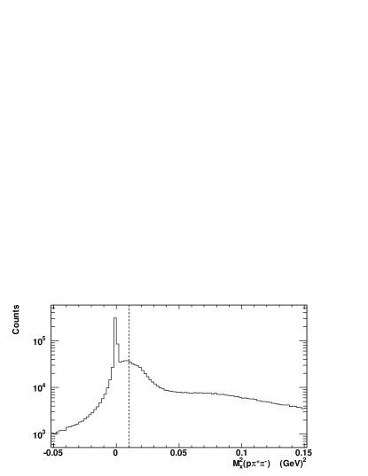
Figure 1: Missing mass squared $(M^{2}_{x})$ for the reaction $\gamma p\to p\pi^{+}\pi^{-}(X)$, where the $\pi^{+}$ was a potentially misidentified kaon. Events above the dotted line at 0.01 GeV² were kept.

The energy lost by charged particles passing through the CLAS detector was accounted for by adjusting the measured particle’s energy according to the average $dE/dx$ losses in the target material, target wall, target scattering chamber, and the start counter scintillators surrounding the target. After correcting for energy loss, several kinematic cuts are applied as described below.

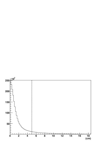
Figure 2: The distance of closest approach between the proton and $\pi^{-}$ shown in cm. The cut used at 5 cm is indicated by the dotted line.

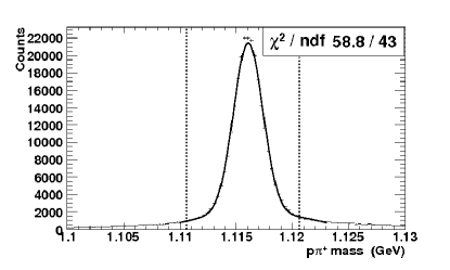
Figure 3: The invariant mass of the $p$-$\pi^{-}$ showing the $\Lambda$ peak with a Gaussian fit giving a $\sigma=1.3$ MeV. A cut of $\pm 0.005$ GeV around the PDG mass of the $\Lambda$ is used indicated by the dotted lines.

Due to the finite resolution of the measured velocity and momentum, in addition to particle decay-in-flight, it is possible that some pions could be misidentified as kaons. To clean up the kaon signal for the analysis, it is common to recalculate the energy of the identified kaon using the mass of the pion. Then the missing mass squared is studied for the reaction $\gamma p\rightarrow p\pi^{+}\pi^{-}(X)$, where the $\pi^{+}$ is actually identified by the above mass cuts as a $K^{+}$. A spike at zero mass squared indicates that the reaction $\gamma p\rightarrow p\pi^{+}\pi^{-}$ is prominent. Most particle misidentified events can be removed by cutting slightly above zero, as shown in Fig. 1. The events above 0.01 GeV² are kept as a cleaner sample of the $\gamma p\rightarrow pK^{+}\pi^{-}(X)$ events. Reactions involving decays such as $\rho\to\pi^{+}\pi^{-}$, where the $\pi^{+}$ is mistakenly identified as a $K^{+}$, are vastly reduced by this cut.

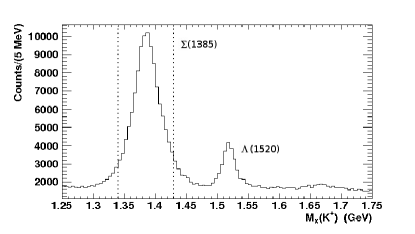
Figure 4: Missing mass for the reaction $\gamma p\to K^{+}(X)$, for events passing the cut on the $\Lambda$ mass. The dotted lines show the 1.34 GeV to 1.43 GeV cut used to select the $\Sigma(1385)$.

The four-momentum of the detected $\Lambda$ was reconstructed from the proton and $\pi^{-}$ four-momenta. The distance of closest approach (DOCA) from the proton and $\pi^{-}$ four-momenta is found and restricted to be less than 5 cm (see Fig. 2). A Gaussian fit to the $p\pi^{-}$ invariant mass peak shown in Fig. 3 resulted in a $\sigma=1.3$ MeV, which is consistent with the instrumental resolution. After restricting the $\Lambda$ mass to be $1.1157\pm 0.005$ GeV, the remaining events were used to construct the missing mass off the $K^{+}$, giving the excited-state hyperon mass spectrum shown in Fig. 4.

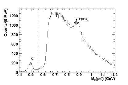
Figure 5: Missing mass for the reaction $\gamma p\to\Lambda(X)$ for events passing cuts on the $\Lambda$ and $\Sigma^{*}$ masses. The dotted line at 0.55 GeV shows the cut used to remove the $\gamma p\to K^{+}\Lambda$ channel. (A looser timing cut was used to illustrate that these accidentals are at the $K^{+}$ mass.)

After making a cut on the $\Sigma^{*}$ peak from 1.34-1.43 GeV, as shown in Fig. 4, one can study the missing mass off of the $\Lambda$, such that $\gamma p\to\Lambda(X)$, shown in Fig. 5. Small peaks are seen at the mass of the kaon and the $K^{*}(892)$. The kaon peak is from exclusive $\gamma p\to K^{+}\Lambda$ production due to accidentals under the TOF peak, and can easily be cut out. The dotted line shows the $M_{x}(\Lambda)>0.55$ GeV event selection used to eliminate this background.

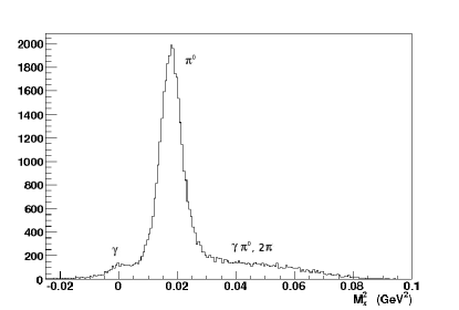
Figure 6: Missing mass squared for the reaction $\gamma p\to K^{+}p\pi^{-}(X)$ after all kinematic cuts.

After including all of the cuts listed above, the missing mass of the reaction $\gamma p\to K^{+}\Lambda(X)$ is shown in Fig. 6. A very prominent peak is seen at the mass of the $\pi^{0}$ with a very small number of counts about zero missing mass due to the EM decay. The counts above the $\pi^{0}$ peak are mostly due to the $\gamma p\to K^{+}\Sigma^{0}(X)$ reaction from photoproduction of higher-mass hyperons.

A small fraction of the events near zero missing mass in the spectrum of Fig. 6 come from accidentals and double bremsstrahlung. In the case of double bremsstrahlung it is possible for false EM decay signals caused by the reaction $\gamma_{1}+\gamma_{2}p\to K^{+}\Lambda+\gamma_{1}$ to mimic the final state of interest $\gamma p\to K^{+}\Lambda\gamma$. The $\gamma_{1}$ from double bremsstrahlung will point down the $z$-axis (along the beam), which can also occur if the event is accidental or due to inefficiencies in the tagger plane from incorrect electron selection. By calculating the transverse missing momentum ($P_{xy}^{2}=P^{2}_{x}+P^{2}_{y}$), it is possible to eliminate double bremsstrahlung. The peak at small values in the distribution in Fig. 7 was removed by requiring $P^{2}_{xy}>0.0009$ GeV² as illustrated by the dashed line. Clearly the effect is quite small, however this step is critical for an accurate measure.

Figure 7: (A) Transverse missing momentum and (B) transverse missing momentum squared for the reaction $\gamma p\to K^{+}\Lambda(X)$. The dashed line shows the cut used at $P^{2}_{xy}>0.0009$ GeV².

In Fig. 6 the tail of the $\pi^{0}$ peak continues into the zero missing mass region. Resolving the two contributions with a simple Gaussian fit does not give systematically consistent results. A technique involving kinematic fitting is required to separate the background from the events of interest, as well as to separate the $\pi^{0}$ events from the radiative signal.

III Simulations

A Monte Carlo simulation of the CLAS detector was performed using GEANT geant , set up for the $g11$ run conditions. Events were generated for the radiative channel ($\Sigma^{0}(1385)\rightarrow\Lambda\gamma$), the normalization reaction ($\Sigma^{0}(1385)\rightarrow\Lambda\pi^{0}$), and several background reactions; see Table 2 for a complete list. Using the data as a guide, the photon beam energy dependence of $K^{+}$ production and the $K^{+}$ angular dependence were used iteratively to tune the Monte Carlo to match the data. After reconstruction, the Monte Carlo momentum distributions for the proton, $\pi^{-}$, and $K^{+}$ matched (within error bars) to that of the data. The generated Monte Carlo events were analyzed using the same analysis procedure used for the data.

After studying the various channels of interest and background, a constant $t$-slope ($d\sigma/d\Omega\sim e^{-bt}$) of $b=$2.0 GeV^-2 was used for the generated $\gamma p\to K^{+}\Lambda(1405)$ channel. The form of the angular distributions of the cross section from data were used in the generator to produce all the $\Sigma^{*}$ simulations.

IV Kinematic Fitting

The kinematic fitting employed in this analysis technique takes advantage of the information in the measured kinematic variables and their uncertainties to fit constraints of energy and momentum conservation, thereby improving the measured quantities using constraint equations. This procedure is useful to improve the separation of signal from background. The method of Lagrange multipliers is the approach implemented here to fit the constraints with a least squares criteria keller .

Assume there are $n$ independently measured data values $y$, which in turn are functions of $m$ unknown variables $q_{i}$, with $m\leq n$. The condition that $y=f_{k}(q_{i})$ is introduced, where $f_{k}$ is a function dependent on the data points that are being tested for each $k$ independent variable at each point.

Because each $y_{k}$ is a measurement with a corresponding standard deviation $\sigma_{k}$, the equation $y_{k}=f_{k}(q_{i})$ cannot be satisfied exactly for $m<n$. It is possible to require that the relationship be satisfied by defining the $\chi^{2}$ relation such that

$$\chi^{2}=\sum_{k}{{(y_{k}-f_{k}(q))}^{2}\over{\sigma_{k}^{2}}},$$ (3)

and require that the preserved values are $q_{i}$, which are the values of $q$ that minimize $\chi^{2}$.

The unknowns are divided into a set of measured variables ($\vec{\eta}$), such as the measured momentum components, and unmeasured variables ($\vec{u}$), such as the missing momentum or the four-vector of an undetected particle in the reaction. The variable $\mathcal{L}_{i}$ is introduced to be used for each constraint equation. The Lagrange multipliers ($\mathcal{L}_{i}$) are used to write the equation for $\chi^{2}$ for a set of constraint equations $\mathcal{F}$ such that,

$$\chi^{2}(\vec{\eta},\vec{u},\mathcal{L})=(\vec{\eta}_{0}-\vec{\eta})^{T}V^{-1}(\vec{\eta}_{0}-\vec{\eta})+2\mathcal{L}^{T}\mathcal{F}(\vec{\eta},\vec{u}),$$ (4)

where $\vec{\eta}_{0}$ is a vector of initial measured quantities and $V^{-1}$ is the inverse of the covariance matrix containing all of the resolutions and correlations of the measured variables from the drift chamber tracking for each charged particle.

The $\chi^{2}$ minimization occurs by differentiating $\chi^{2}$ with respect to each of the variables, while linearizing the constraint equations and obtaining improved measured values from the fit. These values are used as the input for a series of iterations. The iteration procedure is continued until the difference in magnitude between the current $\chi^{2}$ and the previous value is smaller than $\Delta\chi^{2}_{test}$ ($\leq$0.001).

The implemented covariance matrix $V$ was corrected for multiple scattering and energy loss in the target cell, the scattering chamber, and the start counter. These corrections to the diagonal terms in the covariance matrix are applied according to the distance each charged particle travels through the corresponding material.

V Analysis Procedure

A useful kinematic fit for a topology that has a particle that is not detected is the 1C fit. Such a fit requires that a missing mass hypothesis be used to constrain the detected four-momentum, leading to three unknowns from the non-detected particle momentum and four constraints from conservation of energy and momentum. To ensure only high quality $\Lambda$ events, an additional constraint can be implemented on the proton and $\pi^{-}$ tracks to constrain the invariant mass to be the known mass of the $\Lambda$. After the detected particle tracks are kinematically fit, the events can be filtered with a confidence level cut. In this fit there are three unknowns ($\vec{p}_{x}$) and five constraint equations, four from conservation of energy and momentum and the additional invariant mass condition. No additional constraints are required. This makes it a 2C kinematic fit.

To separate the contributions of the $\Sigma^{*0}$ EM decay and the strong decay, the events were fit using the hypotheses for each topology with the constraint equations,

$$\mathcal{F}=\left[\begin{array}[]{c}(E_{\pi}+E_{p})^{2}-(\vec{p}_{\pi}+\vec{p}_{p})^{2}-M_{\Lambda}^{2}\\ E_{\text{beam}}+M_{p}-E_{K}-E_{p}-E_{\pi}-E_{X}\\ \vec{p}_{\text{beam}}-\vec{p}_{K}-\vec{p}_{p}-\vec{p}_{\pi}-\vec{p}_{X}\end{array}\right]=\vec{0},$$ (5)

where $\vec{p}_{X}$ and $E_{X}$ are the momentum and energy of the undetected $\pi^{0}$ or $\gamma$.

To test the functionality of the kinematic fit used to separate the radiative signal from the overwhelming $\pi^{0}$ background, the probability density function keller is used to fit the resulting $\chi^{2}$ distribution. The additional constraint on the invariant mass of the $\Lambda$ takes the probability density function from the more difficult to fit one degree of freedom $\chi^{2}$ distribution (containing a singularity) to the more manageable two degrees of freedom. The fit function takes the form,

$$f(\chi^{2})=\frac{P_{0}}{2}e^{-P_{1}\chi^{2}/2}+P_{2},$$ (6)

where $P_{2}$ is a background term, $P_{1}$ is a quantitative closeness parameter (which gives a measure of how close the distribution in the histogram is to the ideal theoretical $\chi^{2}$ distribution), and $P_{0}$ is for normalization. For a kinematic fit to a missing $\gamma$ with significant background contamination from the $\pi^{0}$, the $\chi^{2}$ distribution will be highly distorted. The ideal $P_{1}$ from a fit to a $\chi^{2}$ distribution with no background is determined from simulations. The deviation of the $P_{1}$ fit parameter from the ideal $P_{1}$ is used as an indicator of the signal to background contribution going into the kinematic fit under the radiative hypothesis and how effective a confidence level cut is expected to be for that given deviation.

Using the $\pi^{0}$-hypothesis for the kinematic fit, the $\chi^{2}$ distribution follows the trend of the probability density function for two degrees of freedom from Eq. (6), see Fig. 8A. The confidence level in Fig. 8B is reasonably flat for the vast majority of events. The spike at zero confidence level in Fig. 8B is from events that do not satisfy the hypothesis in the kinematic fit.

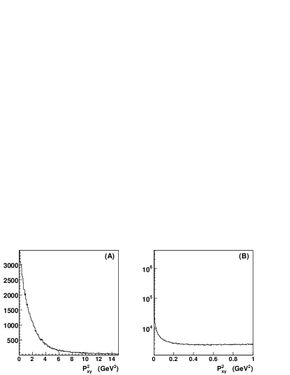
Figure 8: (A) $\chi^{2}$ distribution and (B) confidence level distribution for a missing $\pi^{0}$ hypothesis in the kinematic fit.

For the $\gamma$-hypothesis, without any cuts to reduce the $\pi^{0}$ background, the $\chi^{2}$ distribution is not consistent with the expected probability density function for a 2C fit. Simulations indicate that the $P_{1}$ parameter should be $P_{1}\sim 0.9$, but due to the sensitive nature of the $\chi^{2}$ distribution for two degrees of freedom, a fit to obtain the $P_{1}$ parameter does not return a realistic value. This can be seen in the distorted shape of the distribution in Fig. 9A. Additionally, the confidence level distribution rises up near the low confidence end (Fig. 9B) and is clearly not as flat as the distribution in Fig. 8B. This is an indication that the vast majority of data being kinematically fit at this stage are not satisfying the base assumption of a massless missing particle. This suggests that, even with a high confidence level cut, there is still an overwhelming amount of $\pi^{0}$ events leaking through. However, it is possible to take an additional step in the kinematic fitting procedure for a cleaner separation.

A two-step kinematic fitting procedure is used to systematically reduce the large $\pi^{0}$ background and optimize the extraction of the number of radiative events. First, a fit to a $\pi^{0}$-hypothesis is done and only the low confidence level ($P^{a}_{\pi}(\chi^{2})$) events are retained, followed by a fit of these candidate events to a $\gamma$-hypothesis and retaining the high confidence level ($P^{b}_{\gamma}(\chi^{2})$) events. Because of the previous kinematic cuts, there should now be primarily a $\pi^{0}$ background and the true EM decay signal. Any other background is expected to be very small relative to the radiative signal and will be accounted for through simulations. By first fitting to a $\pi^{0}$-hypothesis and taking the low confidence level candidates, one reduces the probability that the surviving candidates will have a missing mass of the $\pi^{0}$ before they are fit to a $\gamma$-hypothesis.

The selection of the confidence level cuts $P^{a}_{\pi}(\chi^{2})$ and $P^{b}_{\gamma}(\chi^{2})$ is derived using simulations. After testing the ability to recover various mixed ratios on the order of the expected experimental ratio ($\sim 1\%$), a Monte Carlo (MC) simulation of the data was studied for a given ratio of the $\gamma p\to K^{+}\Sigma^{*0}\to K^{+}\Lambda\pi^{0}$ and $\gamma p\to K^{+}\Sigma^{*0}\to K^{+}\Lambda\gamma$ channels. The optimization occurs when considering both the increase in statistical uncertainty from a higher $P^{a}_{\pi}(\chi^{2})$ cut and the increase in MC ratio “recovery” uncertainty from a lower $P^{a}_{\pi}(\chi^{2})$ cut. The “recovery” uncertainty is defined by the difference in the MC generated ratio and the measured ratio or “recovered” ratio found by analyzing the MC with a given $P^{a}_{\pi}(\chi^{2})$ and $P^{b}_{\gamma}(\chi^{2})$. The final confidence level cut in $P^{b}_{\gamma}(\chi^{2})$ is determined by the fit parameter $P_{1}$ indicating how much $\pi^{0}$ background is left after the $P^{a}_{\pi}(\chi^{2})$ cut. Again, the statistical uncertainty and the MC ratio “recovery” uncertainty are considered in the optimization of the $P^{b}_{\gamma}(\chi^{2})$ cut.

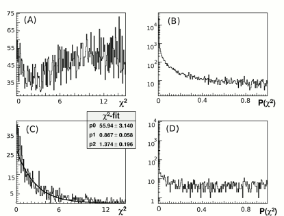
Figure 9: (A) The $\chi^{2}$ distribution and (B) the confidence level distribution for a missing $\gamma$ hypothesis in the kinematic fit before the two-step kinematic fit. (C) The $\chi^{2}$ distribution and the (D) the confidence level distribution for a missing $\gamma$ hypothesis in the kinematic fit after the $P^{a}_{\pi}(\chi^{2})<1\%$ cut.

The results of the optimization study indicate that a confidence level cut of $P^{a}_{\pi}(\chi^{2})<1\%$ sufficiently reduces the $\pi^{0}$ background so that a $P^{b}_{\gamma}(\chi^{2})>10\%$ cut can be used to isolate the radiative signal in the kinematic fit to $\gamma$.

After the two-step kinematic fitting procedure, one can again study the $\gamma$-hypothesis $\chi^{2}$ fit. It now looks more like a standard distribution for two degrees of freedom, returning a value of $P_{1}=0.87\pm 0.06$, see Fig. 9C. The confidence level now appears relatively flat in Fig. 9D, as it should. This is an indication that an improvement has been made on the quality of candidates going into the fit with respect to the hypothesis. This gives some assurance that the candidates going into the secondary fit can be accurately filtered with a confidence level cut.

To ensure the quality of the $\pi^{0}$ extraction, the same two-step kinematic fitting procedure is done by first fitting to a $\gamma$ hypothesis and taking the low confidence level $P^{a}_{\gamma}(\chi^{2})$ candidates, then fitting to the $\pi^{0}$ hypothesis and taking only the high confidence level $P^{b}_{\pi}(\chi^{2})$ candidates.

Once the confidence level cuts are optimized for extracting both the $\pi^{0}$ and radiative signal, the final selected candidates for each case can be seen in the missing mass spectrum, see Fig. 10. The extracted counts are shown for (A) the $\pi^{0}$, (B) the electromagnetic signal, and (C) together in the full spectrum of the missing mass squared. The final raw yields taken directly from the kinematic fit are $n_{\gamma}=635$ and $n_{\pi}=13950$.

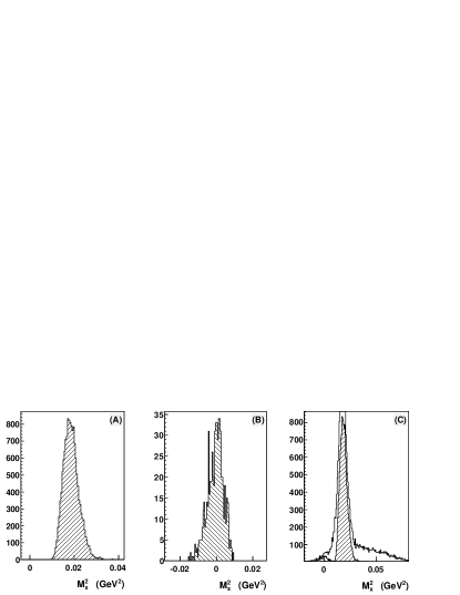
Figure 10: (A) The $n_{\pi}$ counts extracted using the confidence level cuts $P^{a}_{\gamma}<1\%$ and $P^{b}_{\pi}>10\%$. (B) The $n_{\gamma}$ counts extracted using the confidence level cuts $P^{a}_{\pi}<1\%$ and $P^{b}_{\gamma}>10\%$. (C) The counts $n_{\pi}$ and $n_{\gamma}$ shown in the spectrum before any kinematic fit.

Table 2: Acceptances (in units of $10^{-3}$) for the channels used in the calculation of the branching ratio. Here there is a $P^{a}(\chi^{2})<1\%$ confidence level used with a $P^{b}(\chi^{2})>10\%$ cuts. The uncertainties listed are statistical only.

Reaction	$A_{\pi}$	$A_{\gamma}$	$A_{\gamma\pi}$
$\Lambda(1405)\rightarrow\Sigma^{0}\pi^{0}$	0.0495$\pm$0.0031	0.001$\pm$0.0001	1.189$\pm$0.019
$\Lambda(1405)\rightarrow\Sigma^{+}\pi^{-}$	0.029$\pm$0.002	0.0013$\pm$0.0001	0.0078$\pm$0.001
$\Lambda(1405)\rightarrow\Lambda\gamma$	0.0011$\pm$0.0001	1.65$\pm$0.031	0.0223$\pm$0.002
$\Lambda(1405)\rightarrow\Sigma^{0}\gamma$	0.170$\pm$0.012	0.191$\pm$0.009	0.437$\pm$0.013
$\Sigma(1385)\rightarrow\Lambda\pi$	1.421$\pm$0.0278	0.0321$\pm$0.002	0.0312$\pm$0.002
$\Sigma(1385)\rightarrow\Sigma^{+}\pi^{-}$	0.161$\pm$0.01	0.00254$\pm$0.001	0.00138$\pm$0.0006
$\Sigma(1385)\rightarrow\Lambda\gamma$	0.0184$\pm$0.002	2.335$\pm$0.039	0.0704$\pm$0.005
$\Sigma(1385)\rightarrow\Sigma^{0}\gamma$	0.191$\pm$0.011	0.058$\pm$0.0001	0.225$\pm$0.015
$\Lambda K^{*+}\rightarrow K^{+}\pi^{0}$	0.213$\pm$0.010	0.010$\pm$0.006	2.931$\pm$0.051
$\Lambda K^{*+}\rightarrow K^{+}\gamma$	0.0022$\pm$0.0001	0.158$\pm$0.003	2.351$\pm$0.046

The $\pi^{0}$ leakage into the $\gamma$ channel is the dominant correction to the branching ratio. The final result also needs to be corrected for backgrounds, such as $K^{*}\to K^{+}X$ and decays to $\Sigma^{+}\pi^{-}$, as well as the contributions from $\Lambda(1405)\to\Lambda\gamma$. Taking these backgrounds into consideration, and following the notation of Taylor et al. Taylor , the branching ratio $R=N(\Lambda\gamma)/N(\Lambda\pi)$ is

$$R = \frac{1}{\Delta n_{\pi}A^{\Sigma}_{\gamma}(\Lambda\gamma)-\Delta n_{\gamma}A^{\Sigma}_{\pi}(\Lambda\gamma)}$$ (7)

$$\times\left[\Delta n_{\gamma}\left(A^{\Sigma}_{\pi}(\Lambda\pi)+\frac{R^{\Sigma\pi}_{\Lambda\pi}}{2}A^{\Sigma}_{\pi}(\Sigma\pi)\right)\right.$$

$$\left.-\Delta n_{\pi}\left(A^{\Sigma}_{\gamma}(\Lambda\pi)+\frac{R^{\Sigma\pi}_{\Lambda\pi}}{2}A^{\Sigma}_{\gamma}(\Sigma\pi)\right)\right],$$

where terms starting with $A$ are acceptance factors (given below) and

$$\Delta n_{\pi} = n_{\pi}-N_{\pi}(\Lambda^{*}\rightarrow\Sigma^{+}\pi^{-})-N_{\pi}(\Lambda^{*}\rightarrow\Sigma^{0}\pi^{0})$$ (8)

$$-N_{\pi}(\Lambda^{*}\rightarrow\Sigma^{0}\gamma)-N_{\pi}(\Lambda^{*}\rightarrow\Lambda\gamma)$$

$$-N_{\pi}(K^{*}\rightarrow K\pi^{0}),$$

$$\Delta n_{\gamma} = n_{\gamma}-N_{\gamma}(\Lambda^{*}\rightarrow\Sigma^{+}\pi^{-})-N_{\gamma}(\Lambda^{*}\rightarrow\Sigma^{0}\pi^{0})$$ (9)

$$-N_{\gamma}(\Lambda^{*}\rightarrow\Sigma^{0}\gamma)-N_{\gamma}(\Lambda^{*}\rightarrow\Lambda\gamma)$$

$$-N_{\gamma}(K^{*}\rightarrow K\gamma),$$

with $n_{\gamma}$ ($n_{\pi}$) equal to the yield of the kinematic fits, representing the measured number of photon (pion) candidates. In the notation used, lower case $n$ represents an observed number of counts, while upper case $N$ represents the acceptance corrected or derived quantities. Here the $\pi$ and $\gamma$ subscripts indicate the kinematic fit hypothesis and the decay channel is shown in parentheses (note that $\Lambda^{*}$ denotes the $\Lambda(1405)$). These corrections are necessary to take into account due to the fact that the background underneath the $\Sigma(1385)$ is not zero, which could lead to an over-counting of the $\Sigma(1385)$ contribution. For the detector acceptance, the notation has the pion (photon) hypothesis from the $\Sigma(1385)$ decay given by $A^{\Sigma}_{\pi}$ ($A^{\Sigma}_{\gamma}$), so that $A^{\Sigma}_{\gamma}(\Lambda\pi)$ denotes the relative leakage of the $\Sigma^{*0}\to\Lambda\pi$ decay channel into the $\Lambda\gamma$ extraction and $A^{\Sigma}_{\pi}(\Lambda\gamma)$ denotes the relative leakage of the $\Lambda\gamma$ decay channel into the $\Lambda\pi$ extraction. The form of the ratio given in Eq. (7) is developed in more detail in the Appendix.

VI Background Contributions

Table 2 lists all decay channels taken into consideration and the value of the acceptance for the confidence level cuts $P^{a}_{\pi}(\chi^{2})<1$% followed by $P^{b}_{\gamma}(\chi^{2})>10$% for the $\gamma$-hypothesis and $P^{a}_{\gamma}(\chi^{2})<1$% followed by $P^{b}_{\pi}(\chi^{2})>10$% for the $\pi^{0}$-hypothesis. To use these acceptance terms to correct the signal yields, an estimate of the number $n_{\Lambda}$ for the $\Lambda(1405)$ in the event sample is required. The corrections for the $\gamma$ channel are given by

$$N_{\gamma}(\Lambda^{*}\rightarrow\Lambda\gamma) = {A^{\Lambda}_{\gamma}(\Lambda\gamma)BR(\Lambda^{*}\rightarrow\Lambda\gamma)n_{\Lambda}\over A^{\Lambda}_{\gamma\pi}(\Sigma^{0}\pi^{0})+A^{\Lambda}_{\gamma\pi}(\Sigma^{+}\pi^{-})},$$ (10)

$$N_{\gamma}(\Lambda^{*}\rightarrow\Sigma^{0}\gamma) = {A^{\Lambda}_{\gamma}(\Sigma^{0}\gamma)BR(\Lambda^{*}\rightarrow\Sigma^{0}\gamma)n_{\Lambda}\over A^{\Lambda}_{\gamma\pi}(\Sigma^{0}\pi^{0})+A^{\Lambda}_{\gamma\pi}(\Sigma^{+}\pi^{-})},$$ (11)

$$N_{\gamma}(\Lambda^{*}\rightarrow\Sigma^{0}\pi^{0}) = {A^{\Lambda}_{\gamma}(\Sigma^{0}\pi^{0})n_{\Lambda}\over A^{\Lambda}_{\gamma\pi}(\Sigma^{0}\pi^{0})+A^{\Lambda}_{\gamma\pi}(\Sigma^{+}\pi^{-})},$$ (12)

$$N_{\gamma}(\Lambda^{*}\rightarrow\Sigma^{+}\pi^{-}) = {A^{\Lambda}_{\gamma}(\Sigma^{+}\pi^{-})n_{\Lambda}\over A^{\Lambda}_{\gamma\pi}(\Sigma^{0}\pi^{0})+A^{\Lambda}_{\gamma\pi}(\Sigma^{+}\pi^{-})},$$ (13)

where $BR$ is the branching ratio for the decay shown, and likewise for the $\pi^{0}$ channel.

Isospin symmetry is assumed so that $BR(\Sigma^{0}\pi^{0})=BR(\Sigma^{+}\pi^{-})=BR(\Sigma^{-}\pi^{+})\approx 1/3$ for the $\Lambda(1405)$ decay channels. The subscript “$\gamma\pi$” denotes the acceptance for events that do not satisfy the confidence level cuts for either hypotheses of the kinematic fit (i.e. it is likely to come from some background reaction). The values for $BR(\Lambda(1405)\to\Lambda\gamma)=5.4\pm 0.2\times 10^{-4}\%$ and $BR(\Lambda(1405)\to\Sigma^{0}\gamma)=2.0\pm 0.1\times 10^{-4}\%$ are taken from Ref. Burkhardt .

Contributions from the $\Sigma\pi$ decay of the $\Sigma^{0}(1385)$ are also considered. The term in Eq. (7) that takes the $\Sigma^{*}\to\Sigma^{+}\pi^{-}$ counts into consideration uses $R^{\Sigma\pi}_{\Lambda\pi}=0.135\pm 0.011$ PDG , with the acceptance for the individual channels subject to the radiative ($\pi^{0}$) hypothesis and denoted as $A^{\Sigma}_{\gamma}(\Sigma\pi)$ ($A^{\Sigma}_{\pi}(\Sigma\pi)$). The $\Sigma^{*}\to\Sigma^{0}\gamma$ decay branch is also considered, however no measured branching ratio currently exists for this channel. The acceptances are very small and using the higher theoretical prediction of the Algebraic model Bijker yielded only negligible contributions to the background.

In order to find $n_{\Lambda}$, one can look at the events for which neither the $\gamma$ nor the $\pi^{0}$ hypothesis is satisfied. The value of $n_{\Lambda}$ is difficult to determine due to the non-Breit-Wigner shape of the $\Lambda(1405)$ decay. A better approach is to use a Monte Carlo simulation to fill the background according to its internal decay kinematics and normalize it to the data such that the MC matches the data, thereby giving an estimate of $n_{\Lambda}$. Figure 11 shows the MC simulation normalized to the data, giving the estimate used for $n_{\Lambda}$. This can be used to correct all backgrounds except for the $K^{*}$. The final estimate found is $n_{\Lambda}=4085$.

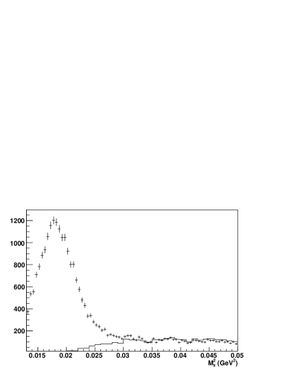
Figure 11: Missing mass of $\gamma p\to K^{+}\Lambda(X)$ for data (points with error bars) and Monte Carlo simulations for the $\gamma p\to K^{+}\Lambda(1405)$ reaction (histogram) normalized to the data.

The $\gamma p\to K^{*0}\Sigma^{+}$ reaction was investigated with the MC simulation and compared with data. This background was determined to have a negligible effect on the final result, since there is no $\Lambda$ in the final state. For the $\gamma p\to K^{*+}\Lambda$ reaction, few events survive all of the cuts. To include corrections for the few events that do survive, an estimate of the $K^{*+}$ background must be established. The correction for this background has the form

$$N_{\pi}(K^{*}\rightarrow K^{+}\pi^{0})=$$ (14)

$$\frac{A_{\pi^{0}}(K^{*+}\to K^{+}\pi^{0})n(K^{*+}\to K^{+}\pi^{0})}{A_{\pi}(K^{*+}\to K^{+}\pi^{0})},$$

where $A_{\pi}(K^{*+}\to K^{+}\pi^{0})$ is the acceptance for the $K^{*+}\to K^{+}\pi^{0}$ channel under the $\pi^{0}$-hypothesis while $A(K^{*+}\to K^{+}\pi^{0})$ is the acceptance of the $K^{*+}\to K^{+}\pi^{0}$ channel which is dependent on the extraction method to obtain the $K^{*+}\to K^{+}\pi^{0}$ counts. $n(K^{*+}\to K^{+}\pi^{0})$ is the estimated number of $K^{*+}\to K^{+}\pi^{0}$ events in the data sample. Similarly, the radiative decay of the $K^{*}$ has the form

$$N_{\gamma}(K^{*}\rightarrow K\gamma)=\frac{3}{2}R(K^{*+}\to K^{+}\gamma)$$ (15)

$$\times\frac{A_{\gamma}(K^{*+}\to K^{+}\gamma)}{A(K^{*+}\to K^{+}\pi^{0})}n(K^{*+}\rightarrow K^{+}\pi^{0}),$$

with $N_{\pi}(K^{*}\rightarrow K\pi^{0})$ from Eq. (LABEL:kcal) and $BR(K^{*+}\to K^{+}\gamma)\simeq 9.9\times 10^{-4}$. An estimate of the number of $K^{*}$ events was obtained by matching the MC simulations to the data. The $K^{*+}\to K^{+}\pi^{0}$ mass distribution has been fit as shown in Fig. 12. In addition a fit is more easily obtained over the range that allows the higher part of the excited state mass spectrum to pass through. Using the resulting Gaussian fit of the $K^{*}$ peak while studying the mass off of the $K^{+}$ for mass windows ranging from 1.34-1.5 GeV to 1.34-1.8 GeV, we are able to extrapolate down to the nominal $\Sigma^{*0}$ mass cut (1.34-1.43 GeV), see Fig. 4. Both methods gave similar results for $n(K^{*+}\to K^{+}\pi^{0})$ used for the background correction in the final ratio. The extrapolated number of $K^{*}\to K^{+}\pi^{0}$ events present were 1207, 14.8 of which passed the $\pi^{0}$-hypothesis.

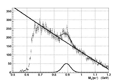
Figure 12: Missing mass off the $\Lambda$ fit with a Gaussian for the mass off of the $K^{+}$ in the window of 1.35-1.5 GeV.

Each background contribution is enumerated in Table 3. The table gives the final breakdown of statistics for each term used in Eqs. (8)-(9) to achieve the corrected counts.

Table 3: Breakdown of statistics for each term in Eqs. (8)-(9) for the $\Lambda(\gamma)$ and $\Lambda(\pi^{0})$ hypotheses. Each listed channel is subtracted from the raw counts found from the kinematic fit in each case. The uncertainties are statistical only. The $\Sigma(1385)\rightarrow\Sigma^{+}\pi^{-}$ contributions are of the order of $10^{-5}$ and smaller and are not included in the table.

Reaction	$\Lambda(\gamma)$	$\Lambda(\pi^{0})$
Raw counts	635	13950
$\Lambda(1405)\rightarrow\Sigma^{0}\pi^{0}$	3.41$\pm$0.36	168.94$\pm$11.65
$\Lambda(1405)\rightarrow\Sigma^{+}\pi^{-}$	4.44$\pm$1.09	98.98$\pm$7.80
$\Lambda(1405)\rightarrow\Lambda\gamma$	3.04$\pm$0.59	0.01$\pm$0.00
$\Lambda(1405)\rightarrow\Sigma^{0}\gamma$	0.13$\pm$0.04	0.12$\pm$0.04
$\Lambda K^{*+}\rightarrow K^{+}\pi^{0}$	0.00$\pm$0.00	27.41$\pm$1.71
$\Lambda K^{*+}\rightarrow K^{+}\gamma$	0.03$\pm$0.00	0.00$\pm$0.00
Corrected counts	623.92$\pm$25.23	13654.56$\pm$118.95

VI.1 RESULTS

The resulting corrected counts $\Delta n_{\gamma}=623.92\pm 25.23$ and $\Delta n_{\pi}=13654.56\pm 118.95$ are used in Eq. (7) to obtain a ratio of 1.42 $\pm 0.12(\text{stat})\%$. The value of each cut was varied to study the effect on the final acceptance corrected ratio. For each variation the new acceptance terms along with the background contributions in Eq. (7) were also recalculated. Each major systematic uncertainty contribution is listed in Table 4, as described in detail below.

Particle identification was done by calculating the velocity for a particle of a given mass, using the measured momentum, and compared with that expected from the measured path length and time-of-flight. Kaons, protons and pions are selected based on the difference of the calculated and measured velocity, called $\Delta\beta$. Variations of the width of the $\Delta\beta$ cut to identify particles gave slightly different values of the final ratio, shown in line (1) of Table 4.

The distance of closest approach (DOCA) cut for the proton and $\pi^{-}$, used to reconstruct the $\Lambda$ momentum, was varied and the stability of the final ratio was examined. In the stable region, corresponding to cuts in the range from 3 cm to 14 cm, the effect on the final ratio is mostly toward higher values, for a larger DOCA cut value, as listed in line (2).

Similarly, the value of the cut on the transverse momentum, $P_{xy}$, was varied. The ratio stabilizes starting at the cut point shown in Fig. 7. A series of cuts were used starting at 0.0009 GeV² and ending at 0.0025 GeV² to study the effect on the final ratio, given by line (3).

The Monte Carlo simulations for various background reactions were done assuming a $t$-dependent slope of 2.0 GeV^-2 for the differential cross sections, based on Regge theory, as described earlier. The value of the $t$-slope is not known precisely, and was varied by $\pm$25%. The effect on the final ratio is shown in line (4).

The number of counts for the $\Lambda(1405)$ and $K^{*}$ backgrounds were determined from fits to the data, using comparisons of shapes from Monte Carlo simulations with the data shown in Figs. 11 and 12. The uncertainty in the number of counts for these backgrounds also affects the final ratio, as shown in lines (5) and (6).

To look at the systematic dependence on the choice of the confidence level cuts, the range defined by the uncertainty for $P_{\pi}^{b}(\chi^{2})$ was checked. As previously described, the Monte Carlo studies lead to the set of optimal $P^{a}_{\pi}$ cuts for a given $P^{b}_{\gamma}$. These optimal cuts allow one to recover, in our standard analysis framework, the ratio of $\Lambda\gamma$ to $\Lambda\pi^{0}$ decay that was used as input into the Monte Carlo simulations. To maximize counting statistics while minimize this uncertainty, the optimal cuts chosen for the analysis were $P^{b}_{\pi}<1\%$ and $P^{b}_{\gamma}>10\%$.

The variation in the branching ratio is studied by selecting the confidence level cuts that lie slightly outside the optimization region found in simulations. In this way the largest range for $P^{b}_{\gamma}$ and $P^{a}_{\pi}$ can be tested while still respecting the cuts derived from the optimization map. Using the full range of ratios in Table 5, the largest and smallest values show the variation for different choices of confidence level cuts, and is listed in line (7).

The branching ratio of the radiative decay of the $\Lambda(1405)$ affects the final result. Because this value is not measured directly, but is taken from the calculated value in Ref. Burkhardt , there is some uncertainty in it. Using the range of values for this branching ratio given in the literature, and recalculating its effect on our result, leads to the uncertainty quoted in line (8).

Table 4 shows a summary of the systematic studies and the higher and lower value of the extracted ratio based on the variations mentioned for each type of uncertainty. The deviation of the ratio is defined by the difference from the quoted ratio of $R=1.42\%$. These deviations, shown in columns 3 and 5 of Table 4, are added in quadrature to give the total systematic uncertainty.

Table 4: Ranges of systematic variation of the final ratio, given in percent, along with the deviation from the central value.

Source	Low Value	Low Deviation	High Value	High Deviation
(1)Particle identification	1.380	$-0.040$	1.490	+0.070
(2)$p\pi^{-}$ DOCA cut point	1.350	$-0.007$	1.480	+0.060
(3)Transverse momentum $P_{xy}$	1.415	$-0.005$	1.433	+0.013
(4)Monte Carlo $t$-dependence	1.380	$-0.040$	1.440	+0.020
(5)$\Lambda(1405)$ counts	1.420	$-0.000$	1.470	+0.050
(6)$K^{*}$ counts	1.420	$-0.000$	1.431	+0.011
(7)$P(\chi^{2})$ cut points	1.388	$-0.032$	1.448	+0.028
(8)$\Lambda(1405)\to\Lambda\gamma$ correction	1.390	$-0.030$	1.420	+0.000
Total Uncertainty		$-0.072$		+0.112

Table 5: Dependence of corrected branching ratio for variation of the confidence level cuts shown.

$P^{b}_{\gamma}(\%)$	$P^{a}_{\pi}(\%)$	R$(\%)$
15	7.5	1.388$\pm$ 0.12
15	5	1.390$\pm$ 0.12
10	5	1.422$\pm$ 0.12
10	1	1.420$\pm$ 0.12
10	0.5	1.421$\pm$ 0.12
5	0.1	1.448$\pm$ 0.12
5	0.05	1.436$\pm$ 0.12

The range of the systematic uncertainty for $R$ in Table 4 is smaller than the statistical uncertainty, in part because each combination of cuts has a large overlap of events (i.e. the same subset of events is present for all choices of cuts). Since the kinematic fit requires a constraint on the $\Lambda$ mass, the kinematic cut on the invariant mass of the $p\pi^{-}$ has no effect.

The final calculated ratio, given in percent, is

$$R^{\Lambda\gamma}_{\Lambda\pi}= \frac{\Gamma[\Sigma^{0}(1385)\rightarrow\Lambda\gamma]}{\Gamma[\Sigma^{0}(1385)\rightarrow\Lambda\pi^{0}]}$$

$$= 1.42\pm 0.12(\text{stat})_{-0.07}^{+0.11}(\text{sys})\%.$$ (16)

Previously published work Taylor on this branching ratio yielded a ratio of $1.53\pm 0.39^{+0.15}_{-0.17}$ %. The value given here is consistent within uncertainties of the previous value, but has smaller uncertainties. The smaller uncertainty is important, as the previous uncertainty was on the same order as the theoretical meson cloud corrections to the EM decay of the $\Delta$. If similar meson cloud corrections are to be proven true for EM decay of the $\Sigma^{*0}$ baryon, then the smaller experimental uncertainty is a significant improvement.

The width for the branching ratio achieved comes from the use of the full width of the $\Sigma^{*0}$, which is $\Gamma(\Sigma^{*0})_{\text{Full}}=36.0\pm 5.0$ MeV with the branching ratio that the radiative signal is being normalized to, which is the $R(\Sigma^{*0}\to\Lambda\pi^{0})=87.0\pm 1.5\%$ PDG . The partial width calculation is then

$$\Gamma_{\Sigma^{*0}\to\Lambda\gamma}= R^{\Lambda\gamma}_{\Lambda\pi}R(\Sigma^{*0}\to\Lambda\pi^{0})\Gamma(\Sigma^{*0})_{\text{Full}}$$

$$= 445\pm 80~{}\text{keV},$$ (17)

where a systematic uncertanty in $R^{\Lambda\gamma}_{\Lambda\pi}$ of $\pm 0.11\%$ is use in combination with the statistical uncertainty. Note that a large part of the uncertainty in Eq. (17) comes from the uncertainty of the full width $\Gamma(\Sigma^{*0})_{\text{Full}}$.

These results verify that the partial width is indeed significantly larger than leading theoretical predictions, indicating that meson cloud effects are an important consideration for future calculations.

The radiative decay $\Sigma^{*0}\to\Lambda\gamma$ is made up of M1 and E2 electromagnetic transitions. Assuming that the E2 amplitude is very small, one can calculate the transition magnetic moment from the measured radiative width Landsberg ,

$$\mu_{\Sigma^{*0}\to\Lambda\gamma}=\sqrt{\frac{2M^{2}_{p}\Gamma_{\Sigma^{*0}\to\Lambda\gamma}}{\alpha p^{3}_{\gamma}}}\mu_{N}=2.75\pm 0.25\mu_{N},$$ (18)

where $p_{\gamma}$ is the photon momentum, $M_{p}$ is the mass of the proton, $\alpha=e^{2}/4\pi\sim 1/137$, and $\mu_{N}$ is the nuclear magneton. The value for the transition magnetic moment is larger than most model predictions even within the experimental uncertainty. For example the naive quark model predicts $\mu_{\Sigma^{*0}\to\Lambda\gamma}=2.28\mu_{N}$ Dhir . We hope that this measurement, along with others to come, will motivate theorists to understand the effect of the meson cloud on the magnetic moment and hence extend our knowledge of the quark wavefunctions in the decuplet baryons.

VII Acknowledgment

The authors thank the staff of the Thomas Jefferson National Accelerator Facility who made this experiment possible. This work was supported in part by the Chilean Comisión Nacional de Investigación Científica y Tecnológica (CONICYT), the Italian Istituto Nazionale di Fisica Nucleare, the French Centre National de la Recherche Scientifique, the French Commissariat à l’Energie Atomique, the U.S. Department of Energy, the National Science Foundation, the UK Science and Technology Facilities Council (STFC), the Scottish Universities Physics Alliance (SUPA), and the National Research Foundation of Korea. The Southeastern Universities Research Association (SURA) operates the Thomas Jefferson National Accelerator Facility for the United States Department of Energy under contract DE-AC05-84ER40150.

.1 Appendix: Ratio Derivation

To calculate the ratio in Eq. (7), the leakage of the $\pi^{0}$ region into the $\gamma$ region (and vice-versa) is the dominant correction. Taking just these two channels into consideration, the number of true counts can be represented as $N(\Lambda\gamma)$ for the $\Sigma^{*0}\to\Lambda\gamma$ channel and $N(\Lambda\pi)$ for the $\Sigma^{*0}\to\Lambda\pi^{0}$ channel. The acceptance under the $\Sigma^{*0}\to\Lambda\gamma$ hypothesis can be written as $A_{\gamma}(X)$, with the subscript showing the kinematic fit hypothesis type and, in parentheses, the channel used in the Monte Carlo for the acceptance. For example, the calculated acceptance for the $\Sigma^{*0}\to\Lambda\gamma$ channel under the $\Sigma^{*0}\to\Lambda\gamma$ hypothesis is $A_{\gamma}(\Lambda\gamma)$, whereas under the $\Sigma^{*0}\to\Lambda\pi^{0}$ hypothesis it is $A_{\pi}(\Lambda\gamma)$. It is now possible to express the measured values $n_{\gamma}$ and $n_{\pi}$ as

$$n_{\gamma}=A_{\gamma}(\Lambda\gamma)N(\Lambda\gamma)+A_{\gamma}(\Lambda\pi)N(\Lambda\pi)$$ (19)

$$n_{\pi}=A_{\pi}(\Lambda\pi)N(\Lambda\pi)+A_{\pi}(\Lambda\gamma)N(\Lambda\gamma).\\$$ (20)

The desired branching ratio of the radiative channel to the $\pi^{0}$ channel using the true counts is then $R=N(\Lambda\gamma)/N(\Lambda\pi)$. This can be obtained by dividing Eq. (19) by Eq. (20) expressed in terms of $R$ as

$$\frac{n_{\gamma}}{n_{\pi}}=\frac{RA_{\gamma}(\Lambda\gamma)+A_{\gamma}(\Lambda\pi)}{A_{\pi}(\Lambda\pi)+RA_{\pi}(\Lambda\gamma)},$$ (21)

then solving for $R$. Expressed in terms of measured values and acceptances, the branching ratio is

$$R=\frac{n_{\gamma}A_{\pi}(\Lambda\pi)-n_{\pi}A_{\gamma}(\Lambda\pi)}{n_{\pi}A_{\gamma}(\Lambda\gamma)-n_{\gamma}A_{\pi}(\Lambda\gamma)}.$$ (22)

Equation (22) uses the assumption that contributions from the $\Sigma(1385)$ will only show up as $\Lambda\gamma$ or $\Lambda\pi^{0}$, neglecting the $\Sigma(1385)\to\Sigma\pi$ channel. An estimate of the total number of $\Sigma(1385)$’s produced using the $\Lambda\pi^{0}$ channel is

$$N(\Sigma^{*0})=\frac{N(\Sigma^{*}\to\Lambda\pi^{0})}{R(\Sigma^{*}\to\Lambda\pi^{0})A(\Sigma^{*}\to\Lambda\pi^{0})},$$ (23)

where $R(\Sigma^{*}\to\Lambda\pi^{0})$ is the branching ratio of the $\Sigma(1385)$ decay to $\Lambda\pi^{0}$ and $A(\Sigma^{*}\to\Lambda\pi^{0})$ is the acceptance for that channel. An estimate of the number of $\Sigma(1385)\to\Sigma^{+}\pi^{-}\to p\pi^{0}\pi^{-}$ counts that would contribute to the $\pi^{0}$ peak is then:

$$N(\Sigma^{*}\to\Sigma^{+}\pi^{-})$$

$$= R(\Sigma^{*}\to\Sigma^{+}\pi^{-})A(\Sigma^{*}\to\Sigma^{+}\pi^{-})N(\Sigma^{*0})$$

$$= \frac{R(\Sigma^{*}\to\Sigma^{+}\pi^{-})A(\Sigma^{*}\to\Sigma^{+}\pi^{-})}{R(\Sigma^{*}\to\Lambda\pi^{0})A(\Sigma^{*}\to\Lambda\pi^{0})}N(\Sigma^{*}\to\Lambda\pi^{0})$$ , (24)

where $R(\Sigma^{*}\to\Sigma^{+}\pi^{-})$ is the branching ratio of the $\Sigma(1385)$ to decay into $\Sigma^{+}\pi^{-}$ and $A(\Sigma^{*}\to\Sigma^{+}\pi^{-})$ is the corresponding acceptance after all cuts. It is possible to simplify the expression by using,

$$R^{\Sigma\pi}_{\Lambda\pi}=\frac{R(\Sigma^{*}\to\Sigma^{\pm}\pi^{\mp})}{R(\Sigma^{*}\to\Lambda\pi^{0})}=0.135\pm 0.011,$$

using the PDG average value PDG . The two charged combinations of the $\Sigma\pi$ decay have equal probability. The Clebsch-Gordon coefficient for the $\Sigma^{*}\to\Sigma^{0}\pi^{0}$ decay is zero, assuming isospin symmetry. The observed counts, expressed in terms of true counts and corresponding acceptances for each hypothesis, becomes

$$n_{\gamma}=A_{\gamma}(\Lambda\gamma)N(\Lambda\gamma)+(A_{\gamma}(\Lambda\pi)+\frac{R^{\Sigma\pi}_{\Lambda\pi}}{2}A_{\gamma}(\Sigma\pi))N(\Lambda\pi)$$ (25)

and

$$n_{\pi}=(A_{\pi}(\Lambda\pi)+\frac{R^{\Sigma\pi}_{\Lambda\pi}}{2}A_{\pi}(\Sigma\pi))N(\Lambda\pi)+(A_{\pi}(\Lambda\gamma))N(\Lambda\gamma).$$ (26)

Solving for $R$ will result in a branching ratio that includes all needed information from the $\Sigma(1385)$. Although the corrections to $R$ from other contamination should be small, it is necessary to include them in the calculation. There is some probability that contamination for these other channels can leak through, and acceptance studies were done for all channels under both the $\Lambda\gamma$ and $\Lambda\pi^{0}$ hypotheses. Results from the acceptance for each hypothesis are shown in Table 2. The branching ratio must include corrections for the $K^{*+}\to K^{+}X$ and the $\Lambda(1405)\to\Sigma\pi$ contamination, as well as a contribution to the numerator of $R$ from $\Lambda(1405)\rightarrow\Lambda\gamma$ decay. The leakage of the $\Sigma\gamma$ channel is assumed to be small relative to the $\Lambda\gamma$ signal. However, this channel is still considered in the acceptance studies, see Table 2.

The branching ratio, taking these backgrounds into consideration, is Eq. (7). The $n_{\gamma}$ ($n_{\pi}$) terms come directly from the yield of the kinematic fits and represent the measured number of photon (pion) candidates. A similar notation is used so that the pion (photon) channel identifications are denoted $A^{\Sigma}_{\pi}(\Sigma^{+}\pi^{-})$ ($A^{\Sigma}_{\gamma}(\Sigma^{+}\pi^{-})$), where $A^{\Sigma}_{\gamma}(\Lambda\pi)$ is the relative leakage of the $\Lambda\pi$ channel into the $\Lambda\gamma$ extraction, $A^{\Sigma}_{\pi}(\Lambda\gamma)$ is the relative leakage of the $\Lambda\gamma$ channel into the $\Lambda\pi$ extraction, $A^{\Sigma}$ is the acceptance strictly for the $\Sigma(1385)$, and $A^{\Lambda}$ is the acceptance for the $\Lambda(1405)$.

Table 2 shows the acceptance terms for the other background channels that are considered in the ratio calculation. The table lists three columns sorted by hypothesis: $A_{\gamma}$, $A_{\pi}$, and the counts that made all other cuts but did not satisfy either the $\gamma$ or $\pi^{0}$ hypothesis, $A_{\gamma\pi}$. The latter is used to obtain an estimate of counts for the specific backgrounds listed.

To obtain the values of $N(\Lambda^{*})$ from Eqs. (10)-(13) that must be subtracted from $n_{\gamma}$ or $n_{\pi}$, the number of observed counts of $\Lambda^{*}\to\Sigma^{0}\pi^{0}$ are used with the acceptances from the third column and the acceptance of the background channel of interest. As an example consider $N(\Lambda^{*}\to\Sigma^{+}\pi^{-})$ under the $\pi$ hypothesis. The number of observed counts $n(\Sigma^{0}\pi^{0})$ above the $\pi^{0}$ peak is given by

$$N(\Lambda^{*})=\frac{n_{\Lambda}}{R(\Lambda^{*}\to\Sigma^{0}\pi^{0})A^{\Lambda}(\Sigma^{0}\pi^{0})}.$$ (27)

The notation $n_{\Lambda}$ here is shorthand for $n(\Sigma^{0}\pi^{0})$, while $R(\Lambda^{*}\to\Sigma^{0}\pi^{0})$ is the probability that the $\Lambda(1405)$ will decay to $\Sigma^{0}\pi^{0}$ and $A^{\Lambda}(\Sigma^{0}\pi^{0})$ is the probability that this decay channel will be observed after all the applied cuts. Isospin symmetry is assumed so that $R(\Sigma^{0}\pi^{0})=R(\Sigma^{+}\pi^{-})=R(\Sigma^{-}\pi^{+})\approx 1/3$ for the $\Lambda(1405)$ decay channels. An estimate of the number of counts in the $\pi^{0}$ peak coming from the reaction $\Lambda^{*}\to\Sigma^{+}\pi^{-}$, using Eq. (27), is

$$N_{\pi}(\Lambda^{*}\to\Sigma^{+}\pi^{-})$$

$$= R(\Lambda^{*}\to\Sigma^{+}\pi^{-})A^{\Lambda}_{\pi}(\Sigma^{+}\pi^{-})N(\Lambda^{*})$$

$$= A_{\pi}^{\Lambda}(\Sigma^{+}\pi^{-})n_{\Lambda}/A_{\gamma\pi}^{\Lambda}(\Sigma^{0}\pi^{0}).$$ (28)

A small adjustment is made to ensure that the $\Lambda^{*}\to\Sigma^{+}\pi^{-}$ contributions are also included by adding in the relative acceptance $A^{\Lambda}(\Sigma^{+}\pi^{-})$ to the denominator. These acceptance terms are found by independently using Monte Carlo for the $\gamma p\to K^{+}\Lambda(1405)\to K^{+}\Sigma^{0}\pi^{0}$ and $\gamma p\to K^{+}\Lambda(1405)\to K^{+}\Sigma^{+}\pi^{-}$ reactions. The counts that survive all cuts but did not satisfy either the $\gamma$ or $\pi^{0}$ hypothesis contribute to $A_{\gamma\pi}$. The leakage for the $\gamma p\to K^{+}\Lambda(1405)\to K^{+}\Sigma^{+}\pi^{-}$ channel is very small but is included for completeness. The final result is

$$N_{\pi}(\Lambda^{*}\to\Sigma^{+}\pi^{-})=\frac{A_{\pi}^{\Lambda}(\Sigma^{+}\pi^{-})n_{\Lambda}}{A_{\gamma\pi}^{\Lambda}(\Sigma^{0}\pi^{0})+A_{\gamma\pi}^{\Lambda}(\Sigma^{+}\pi^{-})}.$$ (29)

From this example it becomes transparent how to express all other associated $\Lambda(1405)$ corrections using only the observed $n_{\Lambda}$ counts and the corresponding acceptance for this channel.

References

- (1) M.A.B. Bég, B.W. Lee and A. Pais, Phys. Rev. Lett. 13, 514 (1964).
- (2) H.R. Rubinstein, F. Scheck, and R.H. Socolow, Phys. Rev. 154, 1608 (1967).
- (3) N. Isgur and G. Karl, Phys. Rev. D 21, 3175 (1980).
- (4) K. Nakamura et al., JPG 37, 075021 (2010).
- (5) V.Yu. Alexakhin et al., Phys. Lett. B 647 8-17 (2007).
- (6) A. Airapetian et al., Phys. Rev. D 75 012007 (2007).
- (7) R.H. Dalitz and D.G. Sutherland, Phys. Rev. 146, 1180 (1966).
- (8) T. Sato and T.S.-H. Lee, Phys. Rev. C 54, 2660 (1996).
- (9) B. Juliá-Díaz, T.-S.H. Lee, T. Sato, and L.C. Smith, Phys. Rev. C 75, 015205 (2007).
- (10) N. Isgur and G. Karl, Phys. Rev. D 20, 1191 (1979).
- (11) S. Taylor et al., Phys. Rev. C 71, 054609 (2005); Erratum: ibid. 72, 039902 (2005).
- (12) J. W. Darewych, M. Horbatsch, and R. Koniuk, Phys. Rev. D 28, 1125 (1983).
- (13) R. Koniuk and N. Isgur, Phys. Rev. D 21, 1868 (1980); Erratum: ibid. 23, 818 (1981).
- (14) M. Warns, W. Pfeil, and H. Rollnik, Phys. Lett. B 258, 431 (1991).
- (15) G. Wagner, A. J. Buchmann, and A. Faessler, Phys. Rev. C 58, 1745 (1998).
- (16) E. Kaxiras, E.J. Moniz, and M. Soyeur, Phys. Rev. D 32, 695 (1985).
- (17) C. L. Schat, C. Gobbi, and N. B. Scoccola, Phys. Lett. B 356, 1 (1995).
- (18) A. Abada, H. Weigel, and H. Reinhardt, Phys. Lett. B 366, 26 (1996).
- (19) T. Haberichter, H. Reinhardt, N. N. Scoccola, and H. Weigel, Nucl. Phys. A 615, 291 (1997).
- (20) R. Bijker, F. Iachello, and A. Leviatan, Annals Phys. 284, 89 (2000).
- (21) M. N. Butler, M. J. Savage, and R. P. Springer, Nucl. Phys. B 399, 69 (1993).
- (22) J. W. C. McNabb et al., Phys. Rev. C 69 042201 (2004).
- (23) R. Bradford et al., Phys. Rev. C 73 035202 (2006).
- (24) M. E. McCracken et al., Phys. Rev. C 81 025201 (2010).
- (25) D. I. Sober et al., Nucl. Instrum. Meth. A 440, 263 (2000).
- (26) B. A. Mecking et al., Nucl. Instrum. Meth. A 503, 513 (2003).
-
(27)
D. Keller, “Techniques in Kinematic Fitting”, Jefferson
Lab, CLAS-NOTE 2010-015. http://www1.jlab.org/ul/Physics/Hall-B/clas/index.cfm?note_year=2010 - (28) CERN-CN Division, GEANT 3.2.1, CERN Program Library W5013 (1993).
- (29) H. Burkhardt and J. Lowe, Phys. Rev. C 44, 607 (1991).
- (30) L. G. Landsberg, and V. V Molchanov, Preprint IHEP 97-42 (1997).
- (31) R. Dhir and R. C. Verma, Eur. Phys. J. A 42, 243 (2009).