Repulsive Fermions in Optical Lattices: Phase separation versus Coexistence of Antiferromagnetism and d-Superfluidity

Abstract

We investigate a system of fermions on a two-dimensional optical square lattice in the strongly repulsive coupling regime. In this case, the interactions can be controlled by laser intensity as well as by Feshbach resonance. We compare the energetics of states with resonating valence bond d-wave superfluidity, antiferromagnetic long range order and a homogeneous state with coexistence of superfluidity and antiferromagnetism. We show that the energy density of a hole $e_{hole}(x)$ has a minimum at doping $x=x_{c}$ that signals phase separation between the antiferromagnetic and d-wave paired superfluid phases. The energy of the phase-separated ground state is however found to be very close to that of a homogeneous state with coexisting antiferromagnetic and superfluid orders. We explore the dependence of the energy on the interaction strength and on the three-site hopping terms and compare with the nearest neighbor hopping t-J model.

I Introduction

The basic mechanism by which attractively interacting fermions can undergo Bardeen-Cooper-Schrieffer(BCS)-type transition through s-wave pairing is now well understood. The copper-oxide (CuO₂) materials are the first example of superconductivity arising from strong repulsive interactions anderson87 . It is argued that the single-band Hubbard model captures the essential physics of on-site repulsion. From variational calculations of the Hubbard model, the mechanism is now understood to be an antiferromagnetic exchange mechanism that favors singlet pairs on different sites leading to pairing in the d-wave channel anderson04 . These calculations show a strong deviation from the standard BCS paradigm with a separation of energy scales for pairing and long range coherence randeria92 ; randeria04 . However, in the absence of a rigorous solution of the Hubbard model in two dimensions, the nature of the ground state, and in particular, whether it is a d-wave superconductor or not is still in debate shastry10 .

Given the difficulties of solving the Hubbard model, another route that is being currently attempted is to turn to ultracold atoms in optical lattices jaksch98 ; greiner02 and use them to emulate Hubbard-like models long studied in the condensed matter physics. Unlike the materials studied in the condensed matter physics in which the interaction strengths are usually fixed, in optical lattices the interactions can be varied over a wide range from weak to strong coupling. Furthermore, in the condensed matter systems changing carrier concentration usually modifies the degree of disorder, while the optical lattices are perfect and clean. Thus, the optical lattices allow direct simulation of one quantum system by another feynman82 . It is hoped that a deeper understanding of superconductivity in repulsive models will suggest mechanisms for driving the transition temperature higher. At present the main bottlenecks faced in creating low entropy states in optical lattices pertain to cooling mechanisms and the role of inhomogeneity introduced by an overall trapping potential. Also, the multi-band effects when strongly interacting fermions are loaded in the optical lattice have to be carefully taken into account diener06 ; buechler10 .

In this article we discuss the problem of repulsively interacting fermions in a square optical lattice. The repulsion can be varied either by increasing the laser intensity or by a Feshbach resonance. For both cases we derive an effective Hamiltonian in the strong coupling regime that is independent of the interaction mechanism. We expect both d-wave superconducting and antiferromagnetic fluctuations to dominate in the ground state.The main question we ask is whether the ground state energetically chooses to phase separate or to stay in a homogeneous state as doping and interactions are changed. In the past, analogous questions were addressed in perovskite compounds such as manganites yunoki98 ; yunoki99 ; dagotto10 . In that case, the phase separation between undoped antiferromagnetic and hole-doped ferromagnetic regions was observed. The origin of the interaction was, however, coulombic repulsion between the localized and mobile electrons.

Our result is that the Hubbard model does show a tendency to phase separate at low hole density. This result is based on a variational theory that compares the energetics for two possible ground states: one that allows phase separation and another with homogeneous coexistence. Here, the possible biases are applied on equal degree to these different scenarios. Given the small difference in energy between the two solutions for phase separation and homogeneous coexistence, other factors may determine the ultimate behavior of the system: for example, long-range interactions may tend to favor coexistence whereas disorder may drive the system toward phase separation. Also, the effect of trapping potential needs to be better understood zhou09 ; mahmud11 .

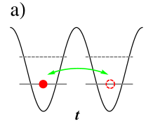
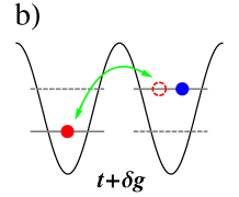
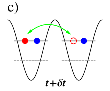
Figure 1: (Color online) Here, we illustrate the effect of having a resonant two-particle state away from the single particle ground state. The hopping amplitudes are essentially given as the overlap of the wave functions of the neighboring sites. Thus, within this “two level” model we can identify three different hopping processes and amplitudes, a) from a single particle state to another single particle state, b) from a two-particle state to a single particle state or the reverse process, and c) from a two-particle state to another two-particle state. Blue and red colors indicate fermions with opposite spins.

II Model

II.1 Hamiltonian

The interactions between fermions in the optical lattices can be controlled in two ways bloch08 ; schneider10 :

i) Laser Intensity controlled: By varying the laser intensity or the optical lattice depth $V_{o}$, we can modify the tunneling rate $t$ of atoms between neighboring sites and the on-site interaction $U$. $t$ and $U$ can be calculated from the band structure theory. In the deep lattice limit, the tunneling rate is given by $t\approx\frac{4}{\sqrt{\pi}}E_{r}\left(\frac{V_{o}}{E_{r}}\right)^{3/4}\exp\left[-2\left(\frac{V_{o}}{E_{r}}\right)^{1/2}\right]$ and the on-site interaction $U\approx\sqrt{\frac{8}{\pi}}ak_{F}E_{r}\left(\frac{V_{o}}{E_{r}}\right)^{3/4}$ bloch08 , where $a$ is the s-wave scattering length that is fixed and $k_{F}$ is the Fermi wave vector. For realizing repulsive fermions, potassium isotope ⁴⁰K can be used where $a$ for hyperfine states is positive ($\approx 160a_{o}$ dalgarno98 ) with $a_{o}$ defined as Bohr radius. Typical $a$ for ⁶Li is $\approx-2000a_{o}$. Here $E_{r}=\frac{h^{2}}{2m\lambda^{2}}$ is the recoil energy of the optical lattice generated by a set of counter-propagating laser beams of wavelength $\lambda$. The expressions above are valid in the non-resonant regime where $k_{F}a\ll 1$. It is then possible to restrict the Hilbert space to a single band Hubbard model given by

$${\cal H}=-t\sum\limits_{<i,j>\sigma}c^{\dagger}_{i,\sigma}c_{j,\sigma}+U\sum\limits_{i}n_{i,+1}n_{i,-1}$$ (1)

where $\sigma=\pm 1$ is the pseudo-spin index. The sums $\langle i,j\rangle$ run over all pairs of nearest-neighbor lattice sites and $n_{i,\sigma}\equiv c^{\dagger}_{i,\sigma}c_{i,\sigma}$. We define doping parameter $x=1-N/N_{latt}$ where $N$ is the total number of fermions of both spin species and $N_{latt}$ is the number of sites in the optical lattice.

ii) Feshbach resonance controlled: By tuning the scattering length $a$ using a magnetic field $B$. Scattering length near resonance takes the form $a=a_{bg}[1-\Delta B/(B-B_{o})]$ where $a_{bg}$ is the background scattering length ($\approx 160a_{o}$ for ⁴⁰K). Also $\Delta B\approx 8$G and $B_{o}\approx 202$ G for ⁴⁰K. Here, the scattering length $a$ can be tuned from the positive values(repulsive) to zero(non-interacting) and to the negative values(attractive). Near the resonance, the interactions can be easily driven into a regime where they exceed the band gap or the energy difference between the lowest two levels in a single lattice site. In this resonant limit the wave function of the two-particle state includes contributions from all excited states and does not reduce to a symmetrized product of the two single particle ground state wave functions. Thus, the minimal set of basis per site should include a single particle ground state as well as a state with double occupancy. Consequently, the overlap of the wave functions for nearest neighbor sites and the hopping amplitudes depend on the particular configuration. This situation is illustrated in the Fig. 1. The physics of the resonant two-particle states introduces two additional parameters $\delta t$ and $\delta g$, which are incorporated into the Hamiltonian in the following form duan05 ; duan08

$$\mathcal{H} = -\sum\limits_{<i,j>\sigma}[t+\delta g(n_{i,\bar{\sigma}}+n_{j,\bar{\sigma}})+\delta t(n_{i,\bar{\sigma}}n_{j,\bar{\sigma}})]c_{i,\sigma}^{\dagger}c_{j,\sigma}$$ (2)

$$+U_{o}\sum\limits_{i}n_{i,+1}n_{i,-1}.$$

Here, $t$ is controlled by the optical lattice depth $V_{o}$ as in Eq. 1. However in the Feshbach resonance case, not just the optical lattice depth $V_{o}$ but also applied magnetic field and other physical parameters of the system determine the value of $U_{o}$. Further discussions below and in the Appendix show that within second order perturbative theory, the Hamiltonians of Eq. 1 and Eq. 2 become analogous with the identification of an effective coupling $U$.

II.2 Our Approach

Given the Hamiltonian, the next step is to determine the quantum phases arising from the strongly repulsive interactions among fermions in two dimensions. At half filling, or zero doping $(x=0)$, the system is a Mott insulator with a finite gap in the charge spectrum and has long range antiferromagnetic order. As the system is doped with holes, antiferromagnetic order decreases and the system develops superfluidity described by a coherent superposition of the resonating valence bond (RVB) singlets anderson87 . Here, each singlet is formed by a pair of opposite fermion species in an orbital state with d-wave spatial symmetry. The question that arises is: What are the characteristics of the quantum phase at small hole density $x$?

In this article, we discuss two possible scenarios:

1) Phase Separation: In this scenario, the system is macroscopically phase separated into regions of antiferromagnetism and superfluidity. We calculate the behavior of the energy density of a hole $e_{hole}(x)$ to check for phase separation.

2) Homogeneous: Here, we consider a single homogeneous phase with coexisting antiferromagnetic and superfluid orders occupying the whole system. We evaluate the energetics of variational states that include both superfluid and antiferromagnetic orders.

By comparing with the more restricted standard t-J model we find that the presence of effective 3-site hopping terms in the full Hamiltonian defined in Eq. 4 leads to a lower energy at non-zero hole density $x$. We also find a stronger tendency to phase separate in the full Hubbard Hamiltonian compared to the more restrictive t-J model.

II.3 Effective Hamiltonian in Strong Coupling

In the large $U/t$ limit, the Hamiltonian in Eq. 1 can be transformed into a block diagonal form where the blocks preserve the total number of the doubly occupied sites and the different blocks are connected by the kinetic/hopping operators (see Appendix). The effective Hamiltonian ${\cal H}_{eff}$ in the strong coupling limit is obtained by a canonical transformationmacdonald88 ; cohen

$${\cal H}_{eff}={\cal V}+{\cal K}_{0}+\frac{1}{U}[{\cal K}_{1},{\cal K}_{-1}]+{\cal O}(1/U^{2})$$ (3)

where the kinetic operator ${\cal K}_{m}$ changes the number of doubly occupied sites by an integer number $m$. ${\cal V}$ is the interaction term. The term given by a commutator (second order term) in Eq. 3 contains two consecutive hoppings. Since we consider $U/t>>0$, we impose the non-double occupancy constraint at each site in order to obtain the low energy Hamiltonian: ${\cal H}_{eff}\rightarrow{\cal P}_{G}{\cal H}_{eff}{\cal P}_{G}$ where ${\cal P}_{G}=\prod\limits_{i}(1-n_{i,1}n_{i,2})$ is the full Gutzwiller projector. As a result, the interaction term $\cal V$ is projected out and the Hamiltonian can be cast as

$${\cal H}_{eff}=-t\sum\limits_{<i,j>\sigma}f^{\dagger}_{i,\sigma}f_{j,\sigma}-\frac{t^{2}}{U}\sum\limits_{<i^{\prime},i>\sigma^{\prime};<i,j>\sigma}f^{\dagger}_{i^{\prime},\sigma^{\prime}}d_{i,\sigma^{\prime}}d^{\dagger}_{i,\sigma}f_{j,\sigma}$$ (4)

The summations run over all independent indices and Eq. 4 is what we call the projected or full Hamiltonian to distinguish it from the more restricted t-J model. In the second sum, we can identify two-site (when $i^{\prime}=j$ ) and three-site (when $i^{\prime}\neq j$) processes. In the t-J model, an additional restriction $i^{\prime}=j$ is imposed such that only two-site exchange is allowed. In Figs. 6 and 7, we show the effects of this constraint. We have introduced definitions: $f^{\dagger}_{i,\sigma}\equiv h_{i,\bar{\sigma}}c^{\dagger}_{i,\sigma}$ the creation operator of a singly occupied site with spin $\sigma$ particle and $d^{\dagger}_{i,\sigma}\equiv c^{\dagger}_{i,\sigma}h_{i,\sigma}n_{i,\bar{\sigma}}$ the creation operator of a doubly occupied site by adding a particle of spin $\sigma$ to a singly occupied site with a spin $\bar{\sigma}$ particle where $h_{i,\sigma}\equiv 1-n_{i,\sigma}$. Rewriting the Hamiltonian in terms of the pseudo-particle operators $f_{i,\sigma}$, $f^{\dagger}_{i,\sigma}$, $d_{i,\sigma}$ and $d^{\dagger}_{i,\sigma}$ makes clear the permitted physical processes. However, these operators do not satisfy the usual anti-commutator nor commutator relations and straightforward theoretical treatment is difficult. Thus, we rely on the variational formalism whose accuracy depends on the chosen ansatz edegger07 ; anderson06 ; sorella02 . In the following section, we discuss the different variational wave functions.

For the fermions near resonance (Eq. 2), the same perturbative Hamiltonian (Eq. 4) is derived with an effective interaction $U$ which has two contributions

$$U=\frac{U_{o}}{(1+\delta g/t)^{2}}.$$ (5)

Here, $U_{o}$ is controlled by the optical lattice depth and the magnetic field while $\delta g/t$ parameter accounts for the appearance of a two-particle state that goes beyond the single band model (see Appendix). The $\delta g$ dependence comes from the allowed virtual processes while the $\delta t$ contribution does not appear in the second order perturbation. As a consequence, we now consider the phase diagram of the Hamiltonian in Eq. 4 as a function of $U/t$ and doping $x$, regardless of the different ways of tuning the interaction $U$.

II.4 Variational Wave functions

1) Phase separated solution using Maxwell construction: Phase separation results from thermodynamic considerations that involve two pure phases. In the following, we give their description leaving the details of Maxwell construction to the section III (Discussion of Results).

The pure superfluid variational state is described by randeria04

$$|\Psi_{SF_{d}}\rangle = {\cal J}{\cal P}_{G}{\cal P}_{N}|SF_{d}\rangle_{MF}$$

$$= {\cal J}{\cal P}_{G}\left[\sum\limits_{\bf k}\alpha_{\bf k}c^{\dagger}_{{\bf k},\sigma}c^{\dagger}_{-{\bf k},\bar{\sigma}}\right]^{N/2}|0\rangle$$

$|\Psi_{SF_{d}}\rangle$ is also called the RVB wave function when Jastrow correlation is set to unity. But as we discuss below, $|\Psi_{SF_{d}}\rangle$ is more general and can also describe a system with long range antiferromagnetism for an appropriate choice of the Jastrow correlations. $|SF_{d}\rangle_{MF}$ is the solution of the simple mean field Hamiltonian of the form: ${\cal H}_{MF}=\sum_{{\bf k}\sigma}\xi_{\bf k}c^{\dagger}_{{\bf k},\sigma}c_{{\bf k},\sigma}+\sum_{\bf k}\Delta_{\bf k}[c^{\dagger}_{{\bf k},\uparrow}c^{\dagger}_{-{\bf k},\downarrow}+h.c.]$. Thus, the parameters $\alpha_{\bf k}$ are given as $\alpha_{\bf k}=\Delta_{\bf k}/\left[\xi_{\bf k}+\sqrt{\xi_{\bf k}^{2}+\Delta_{\bf k}^{2})}\right]$. The d-wave parametrization $\Delta_{\bf k}=\Delta_{d}(\cos k_{x}-\cos k_{y})$ is always energetically favorable in comparison with the s-wave symmetric parametrization $\Delta_{\bf k}=\Delta_{s}$. We get the appropriate $\mu_{var}$ from the number equation $N=\sum\limits_{\bf k}\left[1-\xi_{\bf k}/\sqrt{\xi_{\bf k}^{2}+\Delta_{\bf k}^{2}}\right]$. Independent optimization of $\mu_{var}$ has a negligible effect on the energy. For our fully projected wave function of Eq. LABEL:eqn_rvb, we avoid attaching physical meaning to the parameters $\Delta_{d}$ and $\mu_{var}$. They are taken simply as two independent degrees of freedom in the variational wave function. In order to characterize the quantum phases, the appropriate order parameters that characterize the SF and AF long range order are calculated explicitly in the optimized wave functions. It can be seen that for the wave function of Ref. pathak08 , when long range hopping parameters $t^{\prime}$ and $t^{\prime\prime}$ of $\xi_{\bf k}$ are set to zero, the $\alpha_{\bf k}$ parametrization of the wave function becomes equivalent to that of Ref. giamarchi90 ; himeda99 and Eq. LABEL:eqn_rvb. Unlike the case of high $T_{c}$ materials where the $t^{\prime}$ and $t^{\prime\prime}$ terms are important to describe the correct band structure of the materials, in the context of cold atoms in optical lattices, these extra parameters can be set to zero.

The quantum phase at half filling (zero hole doping) has long range antiferromagnetic (AF) order trivedi90 . For large enough system sizes, a broken SU(2) symmetric ground state becomes likely. In a ground state that has antiferromagnetic long range order, we note that even at zero doping, the singlet correlation accounts for large part of the energy contribution liang88 . Thus, we keep the singlet correlation mechanism of Eq. LABEL:eqn_rvb and adjust the fluctuations around the Neel state with a Jastrow factor that explicitly breaks the SU(2) symmetry: ${\cal J}=e^{m_{af}\Delta_{af}}$. Here,

$$m_{af}=\frac{2}{N_{latt}}\left[\sum\limits_{i\in L_{1}}S_{i}^{z}-\sum\limits_{i\in L_{2}}S_{i}^{z}\right]$$ (7)

is the staggered magnetization operator with $S_{i}^{z}=1/2(n_{i,+1}-n_{i,-1})$. Also, $L_{j}$ is the sub-lattice of index $j$. $\Delta_{af}$ can be interpreted as a local magnetic field that breaks the SU(2) symmetry. Thus, for the zero doping case we are assuming three variational parameters: $\Delta_{d}$, $\Delta_{af}$, and $\mu_{var}$. The improvement in energy due to this choice of the Jastrow factor is $\sim 2\%$ which is much larger than the typical statistical errors. It was found that the optimum value $\Delta_{af}=0.35$ not only produces lower energy but also the correct staggered magnetization trivedi90 .

2) Homogeneous solution with coexistence of antiferromagnetism and superfluidity: A homogeneous state with both the d-wave superfluid and staggered magnetic long range order(denoted by $|AF+SF_{d}\rangle$) is based on the mean field solution giamarchi90 ; himeda99 ; lee97 ; lee03 ; pathak08 . This state is favorable close to the zero hole doping $x=0$ up to a critical $x=x_{c}$. While for $x_{c}\leq x\leq x_{c}^{\prime}$, a pure d-wave superfluid (SF_d) phase is favored. The initial mean field $|AF+SF_{d}\rangle_{MF}$ state is obtained by solving the Hamiltonian

$${\cal H}_{MF} = \sum_{{\bf k}\sigma}\xi_{\bf k}[c^{\dagger}_{{\bf k},\sigma}c_{{\bf k},\sigma}+\xi_{{\bf k}+{\bf Q}}c^{\dagger}_{{\bf k}+{\bf Q},\sigma}c_{{\bf k}+{\bf Q},\sigma}]+\sum_{\bf k}\{{\Delta_{\bf k}[c^{\dagger}_{{\bf k},1}c^{\dagger}_{-{\bf k},2}+h.c.]+\Delta_{{\bf k}+{\bf Q}}[c^{\dagger}_{{\bf k}+{\bf Q},1}c^{\dagger}_{-({\bf k}+{\bf Q}),2}+h.c.]\}}$$ (8)

$$+ \frac{1}{4}\sum_{{\bf k}\sigma}\sigma m_{N}({\bf Q})[c^{\dagger}_{{\bf k}+{\bf Q},\sigma}c_{{\bf k},\sigma}+c^{\dagger}_{{\bf k},\sigma}c_{{\bf k}+{\bf Q},\sigma}]$$

where the $\bf k$ vector is restricted to the reduced Brillouin zone and ${\bf Q}=(\pi,\pi)$. The diagonalization produces two spin density wave bands denoted by subindices $a$ and $b$. The dispersion relations are given as

$$E_{a}({\bf k}) = \frac{\xi_{\bf k}+\xi_{{\bf k}+{\bf Q}}+\sqrt{(\xi_{\bf k}-\xi_{{\bf k}-{\bf Q}})^{2}+m_{N}({\bf Q})^{2}}}{2}$$

$$E_{b}({\bf k}) = \frac{\xi_{\bf k}+\xi_{{\bf k}+{\bf Q}}-\sqrt{(\xi_{\bf k}-\xi_{{\bf k}-{\bf Q}})^{2}+m_{N}({\bf Q})^{2}}}{2}$$ (9)

with $\xi_{\bf k}=-2t(cos(k_{x})+cos(k_{y}))-\mu_{var}$ and $m_{N}({\bf Q})=$ magnetic variational parameter. The corresponding quasiparticle operators are

$$d_{{\bf k},a,\sigma} = \alpha_{\bf k}c_{{\bf k},\sigma}+\sigma\beta_{\bf k}c_{{\bf k}+{\bf Q},\sigma}$$

$$d_{{\bf k},b,\sigma} = -\sigma\beta_{\bf k}c_{{\bf k},\sigma}+\alpha_{\bf k}c_{{\bf k}+{\bf Q},\sigma}.$$ (10)

From these, the ground state ansatz can be written as

$$|\Psi_{AF+SF_{d}}\rangle={\cal J}{\cal P}_{G}{\cal P}_{N}|AF+SF_{d}\rangle_{MF}={\cal J}{\cal P}_{G}\left[\sum\limits_{\bf k}A_{\bf k}d^{\dagger}_{{\bf k},a,+1}d^{\dagger}_{-{\bf k},a,-1}+B_{\bf k}d^{\dagger}_{{\bf k},b,+1}d^{\dagger}_{-{\bf k},b,-1}\right]^{N/2}|0\rangle.$$ (11)

Here, $A_{\bf k}=\Delta_{\bf k}/\left[E_{a}({\bf k})+\sqrt{(E_{a}({\bf k}))^{2}+\Delta_{\bf k}^{2})}\right]$ and $B_{\bf k}=-\Delta_{\bf k}/\left[E_{b}({\bf k})+\sqrt{(E_{b}({\bf k}))^{2}+\Delta_{\bf k}^{2})}\right]$ with d-wave symmetric parametrization $\Delta_{\bf k}=\Delta_{d}(cos(k_{x})-cos(k_{y}))/2$. ${\cal P}_{N}$ projects the wave function into the subspace of total number of particles $N=N_{1}+N_{2}$ with equal populations $N_{1}=N_{2}$. For this variational wave function, the optimization parameters are $\Delta_{d}$, $m_{N}({\bf Q})$, and $\mu_{var}$.

In the hole doped regime, the contribution from particle-particle correlations is small and the hole-hole correlations dominate sorella02 . We assume a Jastrow factor $\cal J$ of the form ${\cal J}=e^{1/2\sum_{i,j}h_{i}h_{j}v_{ij}}$ where the hole density at i-th site is $h_{i}\equiv h_{i,1}h_{i,2}$ and the correlation function is parametrized by $v_{ij}=v/|{\bf r}_{i}-{\bf r}_{j}|$. We find an improvement in energy of the order $\sim 0.1\%$ with $v<0$. Here, the distance between sites $r_{ij}=|{\bf r}_{i}-{\bf r}_{j}|$ must be between the closest images across the tilted boundaries as we later discuss.

III DISCUSSION OF RESULTS

In analogy with the high $T_{c}$ materials, we consider $U$ values in the Eq. 4 centered at $13.33$ (in units of $t$). For the case of the simple single band model (Eq. 1) this $U$ value is solely controlled by the optical lattice depth $V_{o}$ while for the model of Eq. 2, $U$ is controlled by $V_{o}$ as well as by Feshbach resonance(magnetic field). For our discussion, we assume the parametrization of Eq. 5 with $U_{o}=13.33$ and $\delta g/t$ varied. For the non-resonant case, this is just a way of getting different values of $U$, while for the resonant case $\delta g/t$ has physical meaning.

The quantum expectation values are evaluated by Monte Carlo multi-dimensional integration. In order to avoid numerical instabilities along the $k_{x}=k_{y}$ points, we take a patch of lattice sites with the tilted boundary conditions as our system frame kaxiras88 ; randeria04 . The size of the system is $N_{latt}=L^{2}+1$ sites, where $L$ is an odd number. In this way, we also avoid the frustration of the antiferromagnetic phase (one particle of spin +1(-1) should be surrounded by 4 particles of spin -1(+1)) at the half filling and low hole doping limits. The pairing wave function in real space is obtained by Fourier transforming $\phi_{k}=u_{k}/v_{k}$. This function is continuous when crossing the tilted boundaries.

The injection of holes to the antiferromagnetic(AF) phase at half filling destabilizes the AF and beyond a critical hole doping density $x_{c}$, the AF order is completely destroyed giving way to the homogeneous d-wave superfluid (SF_d) (Eq. LABEL:eqn_rvb). There are two possible scenarios of AF $\leftrightarrow$ SF_d transitions considered here: 1) a first order phase transition between AF and SF_d phases as a function of doping. 2) a second order phase transition from a homogeneous $AF+SF_{d}$ phase at low doping densities to the $SF_{d}$ phase. The energetics of this scenario is calculated using the wave function of Eq. 11. In both cases, the pure SF_d phase exists in the hole doping regime $x_{c}<x<x_{c}^{\prime}$. For $x>x_{c}^{\prime}$, the system becomes a normal Fermi fluid (NFF) phase with none of the long range antiferromagnetic and superfluid correlations. In all cases, the s-wave symmetric superfluidity is energetically disfavored.

III.1 Magnetic and Superfluid order parameters

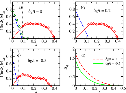
Figure 2: (Color online) Superfluid long range order $\Phi$ (diamonds, continuous line) and antiferromagnetic order parameter $M_{AF}$ (dashed line) at different hole densities and coupling $U$ (plots a-c). These figures correspond to the scenario with phase separation. Here, we assumed the full Hamiltonian of Eq. 4 and the interaction as parametrized by $U=U_{o}/(1+\delta g/t)^{2}$ with $U_{o}=13.33$ in units of $t$ (Eq. 5). In the phase separated region $0<x<x_{c}$ (horizontal dotted line), the order parameters are assumed to depend linearly on $x$, so that $\Phi(x)=\Phi(x_{c})x/x_{c}$ and $M_{AF}(x)=M_{AF}(0)\left[1-x/x_{c}\right]$. For comparison, we also show $M_{AF}(x)$ for the homogeneous phase scenario(circles) at the interaction given by $\delta g/t=0$ (plot a). We find that the order parameters for the phase separation scenario and the homogeneous phase scenario are very close to each other. $U=9.26<U_{o}$ ($\delta g/t=0.2$, plot b) is more favorable for superfluidity with a larger region of phase coexistence, while the opposite is true for $U=53.32>U_{o}$ ($\delta g/t=-0.5$, plot c). There is a distinguishable difference for the optimizing superfluid parameter $\Delta_{d}$ between $\delta g/t=0$ and $\delta g/t=-0.5$ (plot d). However, there is only a small difference for $\Delta_{d}$ between $\delta g/t=0$ and $\delta g/t=0.2$ cases; thus we use the same parametrization for both. The optimum value of the antiferromagnetic parameter $\Delta_{af}$ was $\sim 0.35$ at $x=0$. It has a rather weak dependence on $\delta g/t$ (that is, on $U$).

In order to characterize the quantum phases, we calculate the following long range orders; d-wave order $\Phi=\lim\limits_{j\rightarrow\infty}\phi(j)$. Here, we defined $\phi(j)\equiv\sqrt{2/N\langle\sum\limits_{i}B^{\dagger}_{i+j}B_{i}\rangle}$ with $B^{\dagger}_{i}\equiv 1/2(c^{\dagger}_{i,+1}c^{\dagger}_{i+\hat{x},-1}-c^{\dagger}_{i,-1}c^{\dagger}_{i+\hat{x},+1})$. And the long range order for the staggered magnetization $M_{AF}=\langle m_{af}\rangle$ (Eq. 7). As shown in the Fig. 2, $\Phi$ has a region of favorable d-wave paring at finite hole densities. At zero hole density, we found that the broken SU(2) symmetry wave function produces the correct finite size behavior of $M_{AF}=0.75(2)$ in agreement with previous variational calculations trivedi90 ; pathak08 for the considered system sizes ($N_{latt}=50$ to $226$). These long range orders, however, cannot provide information on the nature of the phase transition (first or second order). In fact, they are shown to be in close agreement for the phase separation and the homogeneous phase cases (Fig. 2). We find that for $U>U_{o}$ where the exchange is suppressed, the superfluid pairing is also suppressed (see Fig. 2), while in the $U<U_{o}$ case the relative mobility $t/U$ of the particles is enhanced and it becomes favorable for d-wave superfluidity.

III.2 Phase separation vs Coexistence at low hole doping

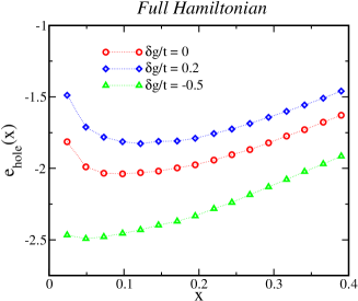
Figure 3: (Color online) Energy density per hole $e_{hole}(x)$ as a function of the hole density $x$ is shown for the full Hamiltonian model. The interaction strengths corresponding to $\delta g/t=-0.5$ ($U/t=53.32$), $0$ ($U/t=U_{o}/t=13.33$) and $0.2$ ($U/t=9.26$) cases are considered. We observe a minimum of $e_{hole}(x)$ at $x=x_{c}>0$ signaling phase separation in the region $0<x<x_{c}$. $x_{c}$ increases monotonically with decreasing $U$ while still remaining in the large $U$ regime. The results are obtained on systems of $N_{latt}=9^{2}+1=82$ lattice sites. The unit of energy is $t$.

In order to characterize the inhomogeneous mixture phase, the thermodynamic considerations are as following: From thermodynamic constraints, the energy per site of the ground state ${\cal E}(x)=E(x)/N_{latt}$ has to be a convex function $\partial^{2}{\cal E}(x)/\partial x^{2}\geq 0$. The range of $x\in(x_{0},x_{1})$ where $\partial{\cal E}(x)/\partial x=constant$ (or $\partial^{2}{\cal E}(x)/\partial x^{2}=0$) implies that the number of holes can be varied while the chemical potential $\mu=\partial{\cal E}(x)/\partial x$ is kept the same. This is a signature of the first order phase transition. In this regime, the system is a mixture of phase $I$ at $x_{0}$ and phase $II$ at $x_{1}$. In our case, $x_{0}=0$ and phase $I$ has antiferromagnetic order(AF) while $x_{c}\equiv x_{1}$ and phase $II$ is the d-wave superfluid(SF_d). In order to check whether there is an interval defined by $x=0$ and $x_{c}>0$, we should check for the flatness of ${\cal E}(x)$ boninsegni08 . However, because we lack the knowledge of the exact mixed phase ground state at all $x$ we use the Maxwell construction: we calculate the energy per hole $e_{h}(x)$ and check for the existence of the minimumemery90 of

$$e_{h}(x)=\frac{{\cal E}_{II}(x)-{\cal E}_{I}(0)}{x},$$ (12)

where ${\cal E}_{I,II}(x)$ are the energy densities of the pure phases (AF and SF_d). This is equivalent to finding $x_{c}$ such that $\frac{\partial{\cal E}_{II}(x)}{\partial x}|_{x_{c}}=\frac{{\cal E}_{II}(x_{c})-{\cal E}_{I}(0)}{x_{c}}$. For all cases considered here, $e_{h}(x)$ has a minimum (Fig. 3) and Maxwell construction with non zero $x_{c}$ is possible. In order to avoid pair breaking effects, we introduce two holes at a time by removing one particle of each species. From Fig. 3, we find that the critical doping strengths are: for $\delta g/t=0$, $x_{c}\approx 0.09$, for $\delta g/t=0.2$, $x_{c}\approx 0.12$, and for $\delta g/t=-0.5$, $x_{c}\sim 0.05$. Correspondingly, the long range orders within the region $0<x<x_{c}$ are proportional to the areas of the pure quantum phases; that is, the AF phase with $x=0$ and SF_d phase with $x=x_{c}$ (see the caption of Fig. 2).

III.3 Ground State Energies

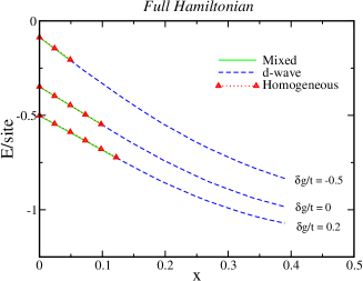
Figure 4: (Color online) The ground state energies of Hamiltonian in Eq. 4 as a function of doping $x$ for various interaction strengths parametrized by $\delta g/t$: $\delta g/t=-0.5$ ($U/t=53.32$), $0$ ($U/t=U_{o}/t=13.33$) and $0.2$ ($U/t=9.26$). Within the region defined by $x\in(0,x_{c})$, we also show the energies corresponding to the first order (continuous line) and the second order (triangle) phase transition scenarios. The energies are shown to be degenerate (within $<0.01\%$ error bars) for the mixed and homogeneous cases. SF_d smoothly transitions to the normal Fermi fluid NFF at $x\gtrsim x_{c}^{\prime}$ ($x_{c}^{\prime}\approx 0.4$) when $\Delta_{d}\rightarrow 0$.The unit of energy is $t$.

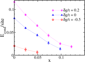
Figure 5: (Color online) Condensation energy per site at different values of $\delta g/t$ for the Hamiltonian of Eq. 4. The unit of energy is $t$. Hole densities $x$ between $0$ and $x_{c}$ are considered. In this case, $x=0$ corresponds to the pure antiferromagnet while $x=x_{c}$ corresponds to the pure superfluid phase. For $0<x<x_{c}$, the condensation energy is that of the homogeneous solution.

The ground state energies for the full Hamiltonian are shown in the Fig. 4. We notice that the mixed phase and the homogeneous phase energies are closely degenerate within the region of $x\in(0,x_{c})$ in all of the considered cases. The kinetic energy has no contribution at zero doping. In this case, the only contribution comes from exchange. As holes are injected to the system, exchange of particles becomes suppressed while the kinetic contribution increases. In the normal phase regime beyond $x_{c}^{\prime}$, most of the contribution to the energy comes from the kinetic term. The composition of energies for the t-J model is shown in the Fig. 8.

From the Fig. 5, we see a monotonically decreasing behavior of the condensation energy $E_{cond}$ which is the difference in energies between the normal state and the state with quantum coherence. Since $E_{cond}$ is at its largest for the pure antiferromagnetic phase, we can argue that once the system is phase separated it would not transition into the homogeneous phase. This would be true even when the superfluid portion of the system is destroyed by thermal fluctuations as long as the antiferromagnetic portion retains its phase coherence. Thus, we argue that the phase separation scenario is more robust than the homogeneous coexistence.

III.4 Comparison of the Full vs t-J models

In the Figs. 6 and 7, a comparison of the full and the t-J Hamiltonians at different values of $\delta g/t$ is given. Both models converge at the zero doping $x=0$ since three-site hopping terms are density suppressed. However, at finite doping, differences arise: as seen in the Fig. 6, the $e_{hole}(x)$ tends to have a slightly larger curvature leading to a clear definition of $x_{c}$. This tendency is more noticeable for $\delta g/t>0$ ($U<U_{o}$). But, for $U<<U_{o}$, the validity of the perturbative Hamiltonian (Eq. 3 and 4) is being compromised. Here, the critical $x_{c}$ seems to be identical for these two models.

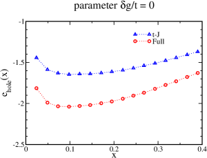
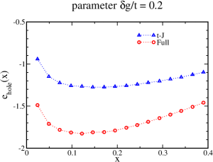
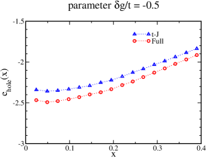
Figure 6: (Color online) Comparison of the energy density per hole $e_{hole}(x)$ for the full and the t-J Hamiltonians at different values of $\delta g/t$: $\delta g/t=-0.5$ ($U/t=53.32$), $0$ ($U/t=U_{o}/t=13.33$) and $0.2$ ($U/t=9.26$). For the full Hamiltonian, the minimum of $e_{hole}(x)$ is more clearly defined signaling greater tendency for phase separation. The unit of energy is $t$.

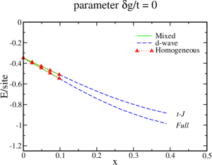
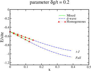
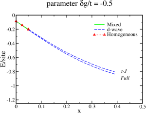
Figure 7: (Color online) Comparison of the ground state energies for the full and the t-J Hamiltonians at different values of $\delta g/t$: $\delta g/t=-0.5$ ($U/t=53.32$), $0$ ($U/t=U_{o}/t=13.33$) and $0.2$ ($U/t=9.26$). The full Hamiltonian includes three-site hopping terms (Eq. 4) that lower the energy relative to the t-J model. At zero hole doping, three-site terms are suppressed and both models converge. The unit of energy is $t$.

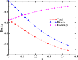
Figure 8: (Color online) Doping dependence of the total, kinetic and exchange energies for the t-J model. The unit of energy is $t$.

IV CONCLUDING REMARKS

We have investigated the appearance of different quantum phases in a system of strongly interacting fermions in the two dimensional optical lattices. We have shown that the interaction strength $U$ has a direct impact on the shape of the phase diagram. In the laboratory, the optical lattice is usually placed within a smoothly varying harmonic trap. Then, the usual shell structure is expected to appear. We have shown that the mixed phase is energetically allowed and possibly more robust than the homogeneous phase.

There are several experimental techniques to measure the quantum correlations: for example, radio frequency techniques to directly measure the excitation spectrum of the Fermi gas are being developed (see Ref. jin08 ). The measurement of the correlations in the noise could also be used, as it was applied to the detection of the Mott insulator phase (see Ref. bloch08 ). Also, Bragg scattering is a scheme that allows the detection of the nodal points in the momentum space hofstetter02 . A connection of the single band model to the resonant regime was made through perturbation theory, although a more elaborate multi-band model might be required for improved description.

We acknowledge support by DARPA BAA 06-19. SP thanks Department of Science and Technology (DST) for funding and APS-IUSSTF Physics Student Visitation Program for travel support. SYC and NT also acknowledge support from ARO W911NF-08-1-0338 and NSF-DMR 0706203. We thank P. Zoller, M. Baranov, and U. Schneider for helpful discussions.

V APPENDIX

For the resonant fermions with $k_{F}a$ large, multi-band effects have to be included. A model by Duanduan05 ; duan08 accounts them by an effective single-band Hubbard-type model. This approach physically corresponds to taking into account only the lowest energy but exact one-particle and two-particle states on each lattice site. For a single-particle state, the corresponding wave function is simply the ground sate wave function in the local potential well. In the strongly interacting limit, the wave function of a two-particle state includes contributions of all excited states and does not reduce to a properly symmetrized product of the two ground state wave functions. As a result, the overlap of the wave functions for nearest neighbor sites and, therefore, the hopping amplitude between them will depend on a particular density configuration (see Fig. 1): The hopping amplitude $t_{01}=t_{10}=t$ for the hop from a singly occupied site to an empty site, will be different from the hopping amplitudes $t_{11}=t_{02}=t_{20}=t+\delta g$ for a hop from a singly occupied site to another singly occupied one and for a reverse hop from a doubly occupied site to an empty one, respectively. This is because the amplitude $t_{01}$ contains the overlap between the two ground state wave functions on the nearest-neighbor sites, while the amplitudes $t_{11}=t_{02}$ are determined by the overlap of the exact two-particle wave function on a site with the product of the ground state wave functions on the same and the nearest-neighbor sites. In turn, the hopping amplitude $t_{12}=t_{21}=t+\delta t$ for a hop from a doubly occupied site to a singly occupied site contains the overlap of the exact two-particle wave functions on nearest-neighbor sites and, hence, will be different from both $t_{01}$ and $t_{11}=t_{02}$. As a result, the Hamiltonian of the extended Hubbard model reads

$$\mathcal{H} = -\sum\limits_{<i,j>\sigma}[t+\delta g(n_{i,\bar{\sigma}}+n_{j,\bar{\sigma}})+\delta t(n_{i,\bar{\sigma}}n_{j,\bar{\sigma}})]c_{i,\sigma}^{\dagger}c_{j,\sigma}$$ (13)

$$+U_{o}\sum\limits_{i}n_{i,+1}n_{i,-1},$$

where the density assisted hopping terms in the kinetic energy is characterized by $\delta g$ and $\delta t$.

The coefficients $\delta g/t$ and $\delta t/t$ depend on the characteristics of the atomic species such as the width (in magnetic field) of the resonance $\Delta B$, the background scattering length $a_{bg}$ and the difference of the atomic magnetic moments between the closed and the open scattering channels $\Delta\mu$. In particular, $\delta g/t$ can be written as $\delta g/t\approx(0.38(V_{o}/E_{r})^{0.25}-1)+\alpha$ (see the Fig. 1 of the Ref. duan05 ). $\alpha$ is a weakly dependent quantity of $V_{o}/E_{r}$ and proportional to $\sqrt{\Delta B|a_{bg}|\Delta\mu}$. Thus, for a given atomic species and a resonant magnetic field, $\delta g/t$ can be tuned over a range of the optical lattice depths.

We define the kinetic operators $\mathcal{K}_{m}$ as

$$\mathcal{K}_{0} = -t\sum\limits_{<i,j>\sigma}h_{i,\bar{\sigma}}c_{i,\sigma}^{\dagger}c_{j,\sigma}h_{j,\bar{\sigma}}$$

$$-(t+2\delta g+\delta t)\sum\limits_{<i,j>\sigma}n_{i,\bar{\sigma}}c_{i,\sigma}^{\dagger}c_{j,\sigma}n_{j,\bar{\sigma}}$$

$$\mathcal{K}_{1} = -(t+\delta g)\sum\limits_{<i,j>\sigma}n_{i,\bar{\sigma}}c_{i,\sigma}^{\dagger}c_{j,\sigma}h_{j,\bar{\sigma}}$$

$$\mathcal{K}_{-1} = -(t+\delta g)\sum\limits_{<i,j>\sigma}h_{i,\bar{\sigma}}c_{i,\sigma}^{\dagger}c_{j,\sigma}n_{j,\bar{\sigma}}$$ (14)

$\mathcal{K}_{m}$ change the number of doubly occupied sites by $m$ and obeys commutation relation $[\mathcal{V},\mathcal{K}_{m}]=mU_{o}\mathcal{K}_{m}$ with $\mathcal{V}=U_{o}\sum\limits_{i}n_{i,+1}n_{i,-1}$)

Here, we have used the usual definition $h_{i,\sigma}\equiv 1-n_{i,\sigma}$. The full Gutzwiller projector can be shown to drop the interaction and the $\delta t$ dependent terms. The effective Hamiltonian after Schrieffer-Wolff transformation is then the same as Eq. 4 with the definition of the effective $U\equiv U_{o}/(1+\delta g/t)^{2}$. In a recent work wang08 on the one dimensional attractive fermionic gas with population imbalance, it was found that the pairing order gets enhanced with $\delta g<0$, while the spin-spin correlation is suppressed. Obviously, due to the difference in the dimensionality (1D vs 2D) and the nature of the interaction (attractive vs repulsive), an intuitive connection is rather complicated.

References

- (1) P. W. Anderson, Scence 235, 1196 (1987).
- (2) P. W. Anderson, P. A. Lee, M. Randeria, T. M. Rice, N. Trivedi, and F. C. Zhang, J. Phys. Cond. Mat. 16, R755(2004).
- (3) M. Randeria, N. Trivedi, A. Moreo, and R. T. Scalettar, Phys. Rev. Lett. 69, 2001 (1992).
- (4) A. Paramekanti, M. Randeria, and N. Trivedi, Phys. Rev. Lett. 87, 217002 (2001). M. Randeria, A. Paramekanti, and N. Trivedi, Phys. Rev. B 69, 144509 (2004).
- (5) C. J. Jia, B. Moritz, C.-C. Chen, B. Sriram Shastry, and T. P. Devereaux, arXiv:1012.4013 (2010).
- (6) D. Jaksch, C. Bruder, J. I. Cirac, C. W. Gardiner, and P. Zoller, Phys. Rev. Lett. 81, 3108 (1998).
- (7) M. Greiner, O. Mandel, T. Esslinger, T. W. Hänsch, and I. bloch, Nature 415, 39 (2002).
- (8) R. Feynman, Int. J. Theor. Phys. 21, 467 (1982).
- (9) R. B. Diener and T.-L. Ho, Phys. Rev. Lett. 96, 010402 (2006)
- (10) H. P. Büchler, Phys. Rev. Lett. 104, 090402 (2010).
- (11) S. Yunoki, J. Hu, A. L. Malvezzi, A. Moreo, N. Furukawa, and E. Dagotto, Phys. Rev. Lett. 80, 845 (1998).
- (12) A. Moreo, S. Yunoki, and E. Dagotto, Science 283, 2034 (1999).
- (13) E. Dagotto, Nanoscale Phase Separation and Colossal Magnetoresistance: The Physics of Manganites and Related Compounds, Springer-Verlag, Berlin Heidelberg (2010).
- (14) Q. Zhou, Y. Kato, N. Kawashima, and N. Trivedi, Phys. Rev. Lett. 103, 085701 (2009).
- (15) K. W. Mahmud, E. N. Duchon, Y. Kato, N. Kawashima, R. T. Scalettar, and N. Trivedi, arXiv:1101.5726 (2011).
- (16) I. Bloch, J. Dalibard, and W. Zwerger, Rev. of Mod. Phys. 80, 885 (2008).
- (17) U. Schneider, PhD. Thesis, Johannes Gutenberg University of Mainz (2010).
- (18) R. Cote, A. Dalgarno, H. Wang, and W. C. Stwalley, Phys. Rev. A 57, R4118 (1998).
- (19) L.-M. Duan, Phys. Rev. Lett. 95, 243202 (2005).
- (20) L.-M. Duan, Europhysics Lett. 81, 20001 (2008).
- (21) A. H. MacDonald, S. M. Girvin, and D. Yoshioka, Phys. Rev. B 37, 9753 (1988).
- (22) C. Cohen-Tannoudji, J. Dupont-Roc, and G. Grynberg, Atom-Photon Interactions, John Wiley & Sons (1992).
- (23) B. Edegger, V. N. Muthukumar, and C. Gros, Advances in Physics 56, 927 (2007).
- (24) B. Edegger, V. N. Muthukumar, C. Gros, and P. W. Anderson, Phys. Rev. Lett. 96, 207002 (2006).
- (25) S. Sorella, et al, Phys. Rev. Lett. 88, 117002 (2002).
- (26) S. Pathak, et al, Phys. Rev. Lett. 102, 027002 (2009).
- (27) T. Giamarchi and C. Lhullier, Phys. Rev. B 43, 12943 (1990).
- (28) A. Himeda and M. Ogata, Phys. Rev. B 60, R9935 (1999).
- (29) N. Trivedi and D. M. Ceperley, Phys. Rev. B 41, 4552 (1990).
- (30) S. Liang, B. Doucot, and P. W. Anderson, Phys. Rev. Lett. 61, 365 (1988).
- (31) T. Lee, and C. Shih, Phys. Rev. B 55, 5983 (1997).
- (32) T. Lee, C.-M. Ho, and N. Nagaosa, Phys. Rev. Lett. 90, 067001 (2003).
- (33) E. Kaxiras and E. Manousakis, Phys. Rev. B 37, 656 (1988).
- (34) M. Boninsegni and N. V. Prokof’ev, Phys. Rev. B 77, 092502 (2008).
- (35) V. J. Emery, S. A. Kivelson, and H. Q. Lin, Phys. Rev. Lett. 64, 475 (1990).
- (36) J. T. Stewart, J. P. Gaebler, and D. S. Jin, Nature 454, 744 (2008).
- (37) W. Hofstetter, J. I. Cirac, P. Zoller, E. Demler, and M. D. Lukin, Phys. Rev. Lett 89, 220407 (2002).
- (38) B. Wang and L.-M. Duan, Phys. Rev. A 79, 043612 (2009).