Classical Effective Field Theory
for
Weak Ultra Relativistic Scattering

Abstract

Inspired by the problem of Planckian scattering we describe a classical effective field theory for weak ultra relativistic scattering in which field propagation is instantaneous and transverse and the particles’ equations of motion localize to the instant of passing. An analogy with the non-relativistic (post-Newtonian) approximation is stressed. The small parameter is identified and power counting rules are established. The theory is applied to reproduce the leading scattering angle for either a scalar interaction field or electro-magnetic or gravitational; to compute some subleading corrections, including the interaction duration; and to allow for non-zero masses. For the gravitational case we present an appropriate decomposition of the gravitational field onto the transverse plane together with its whole non-linear action.
On the way we touch upon the relation with the eikonal approximation, some evidence for censorship of quantum gravity, and an algebraic ring structure on 2d Minkowski spacetime.

1 Introduction

The effective field theory (EFT) approach to General Relativity (GR) GoldbergerRothstein1 borrows ideas from effective quantum field theories and applies them to the two-body post-Newtonian dynamics in classical General Relativity. In addition to contributing insight and a fresh perspective the approach allowed to push forward the state of the art PortoRothstein by computing for the first time the next to leading spin1-spin2 interaction in the effective two-body action.

Most of the ensuing work on the EFT approach centered on the post-Newtonian approximation – see for example NRGR . However, the EFT approach has a very wide applicability range, namely whenever a field theory (not necessarily of gravity) contains two widely separated length (or time) scales CLEFT-caged . Thus far some such applications appeared: a post-Newtonian theory for caged black holes (black holes localized within a compact dimension) caged ; black hole internal degrees of freedom at low frequencies dissip ; new observations on finite size corrections to the radiation reaction force in classical electrodynamics Galley:2010es ; some results on the gravitational two body problem in the extreme mass ratio limit, see GalleyHu1 and continuations of it; and finally see Cannella:2009he for some tests of GR.

In this work we shall present a new classical effective field theory, namely for weak ultra-relativistic scattering, in the context of Einstein’s gravity or more generally any other field theory.

We start in subsection 1.1 by reviewing past work on Planckian scattering including 'tHooft87 ; ACV as a concrete challenge for quantum gravity to address. This part serves as motivation for our work but the ensuing parts are independent of it.

In section 2 we set up the effective field theory and determine its central Feynman rules. The main ingredient is to set the field propagator to be

$$\frac{1}{k_{\perp}^{2}}$$ (1)

This means that the field is instantaneous and transverse. The intuition is that while a particle at rest has a spherical configuration of field strength lines emanating from it, an ultra relativistic boost Lorentz contracts the longitudinal direction, thereby confining the field lines to a transverse pancake attached to the particle’s “nose” (see figure 1). Accordingly the particles interact only at the moment of passing when they each intersect with the other pancake, and the equations of motion degenerate to that instant.

We conclude this section by computing the leading momentum transfer during scattering for several cases of interaction fields: scalar, electromagnetic and gravitational, reproducing the literature value in the latter case. On the way we make use of the light-cone formalism where the dynamics of each particle is nearly Galilean, we define effective ultra-relativistic charges and we define a conserved global charge for the interaction fields. We observe that this theory is analogous to the non-relativistic EFT only in one fewer dimension: the fields propagate instantaneously and the particle dynamics is nearly non-relativistic.

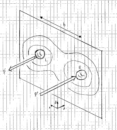
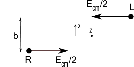
Figure 1: The geometry of the scattering process. Left: 3d geometry at the moment of passing, including equipotential lines. Note that the field lines are Lorentz compressed to the transverse plane. Right: top view. The initial condition parameters are the center of mass energy $E_{cm}$ and the impact parameter $b$. The right moving particle, namely the one moving in the positive $z$ direction, is denoted by R, while the other is denoted by L.

In section 3 we proceed to compute some higher order corrections, present even for linear fields, which are due to non-linearities in the solutions of the equations of motion, where in particular retardation effects must be considered. Setting-up a perturbative theory for ultra-relativistic particles and using the two-body effective action (where the field is integrated out) allows us to find the leading order longitudinal momentum exchange. It comes at second order in the small parameter, while the transverse momentum transfer is of first order, thereby confirming the assumed hierarchy of scales which defines the EFT.

In section 4 we choose a different time for initial conditions thereby changing our “regularization condition” and hence “resumming” and simplifying the perturbation series. This ingredient enables us to proceed to the third order and in particular to resolve the instantaneous interaction and to obtain its duration. This result demonstrates the utility of our formalism.

In section 5 we compute corrections due to non-zero masses, which are controlled by another small parameter. Finally in section 7 we summarize our results and discuss open questions. The appendices contain some conventions and calculations, as well as an algebraic curiosity.

In section 6 we describe the dimensional reduction of the gravitational field onto the transverse plane and its whole non-linear action. The analogue reduction for electromagnetic case is considerably simpler and is treated in section 3.

The EFT in this paper is related to the eikonal approximation in quantum field theory. Actually the latter is the semi-classical approximation corresponding to this EFT. Some of our results including an effective field theory for Planckian scattering appeared elsewhere including in Amati-Ciafaloni-Veneziano[93] ACV93 ; however, we have a different approach: our EFT is purely classical, we define the small parameter and establish power counting rules, we analyze fields other than gravity, and we compute various corrections including the interaction time.

We note that the ultra-relativistic limit is part of the post-Minkowski approximation (see postMink and references therein) where one considers perturbations around a flat space-time due to bodies with arbitrary velocities, possibly relativistic but not ultra-relativistic. However, for our more restricted velocity range we are able to construct an EFT which allows to compute arbitrary higher order corrections, while in the post-Minkowski case so far only a first order correction was demonstrated to be possible.

1.1 Planckian scattering and classical dominance

In order to explore quantum gravity it is natural to consider a gedanken scattering experiment where two gravitationally interacting bodies are scattered (see figure 1), especially when the center of mass energy is Planckian or higher Dray-`tHooft ; 'tHooft87 ; ACV ; ACV93 ; ACV2008 . For simplicity we may assume the particles to be light-like (massless) and point-like. Later we shall study corrections when the masses are non-zero but still much smaller than the energies. We shall also discuss finite-size corrections.

The initial conditions are specified by two parameters

$$E_{cm},~{}b$$ (2)

the center of mass energy, and the impact parameter.

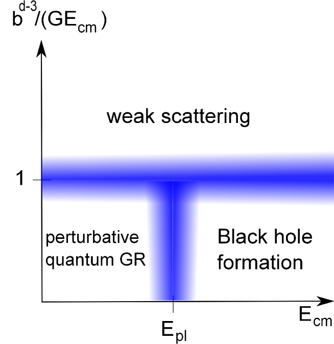
Figure 2: The parameter space for trans-Planckian scattering, demarcating the boundaries between three theoretical regions.

Let us discuss the physics as a function of this parameter space (see figure 2). For generality we consider a general space-time dimension $d$. For $b=0$ we may compare $E_{cm}$ with the Planck energy $E_{Pl}:\simeq\hbar/\left(\hbar G\right)^{1/(d-3)}$ (where $G$ is Newton’s gravitational constant). For large $E_{cm}$ we expect a semi-classical black hole to form, followed by a long period of Hawking evaporation, while for small $E_{cm}$ tree-level quantum GR would be valid (loops are suppressed by $GE_{cm}^{d-2}\sim\left(E_{cm}/E_{Pl}\right)^{d-2}$).

For large $b$ on the other hand, we should compare $b$ with the would-be Schwarzschild radius $R(E_{cm}):=\left(GE_{cm}\right)^{1/(d-3)}$ which is the only other parameter with length dimension. Accordingly large $b$ means $b\gg R(E_{cm})$. In this regime the interaction is dominated by a single field exchange, so having no loops this is essentially classical scattering.

It is interesting to consider varying $b$ from large to small, while keeping $E_{cm}$ fixed and large in Planck units. For large $b$ we have a small attractive deflection. As $b$ is reduced the deflection angle increases together with the deflection time. While (classical) gravitational radiation is weak for weak deflection, it too increases as $b$ is lowered. At some critical (or marginal) $b=b_{c}$ a black hole forms. By dimensional analysis $b_{c}$ must be order one in units of $R(E_{cm})$. We see no reason why the marginal black hole mass would not be zero. That means that at $b_{c}$ all the incoming energy is emitted in the form of gravitational radiation. From general considerations the scattering angle and time diverge in this limit. Recently numerical GR simulations succeeded for the first time in simulating a black hole creation in this process ChoptuikPretorius (and references therein). Incidentally we note that the simulations indicate that the marginal small black hole is very close to extremal spin.

For $b<b_{c}$ the black hole mass is non-zero, and the dependence on $b_{c}-b$ defines a certain characteristic exponent (and the same holds for its angular momentum). After the appearance of a black hole horizon, the black hole relaxes to its stationary form through the classical process of “ringdown” emission of gravitational waves. The ringdown radiation is a smooth continuation of the inspiral radiation.

As $b\to 0$ we know that the colliding light-like shock fronts do not interact until they reach $z=0$. Being at sub-Planckian distance this collision is outside the validity of classical GR, yet we expect most of the energy to be converted to a black hole, and therefore the results of this quantum gravity process would remain hidden behind a horizon. At infinity one observes the Hawking radiation which is semi-classical apart for the last burst of one Planck mass which is an essential quantum gravity effect. Due to Hawking evaporation black hole formation does not necessitate a genuine phase transition (since for all $b$ eventually all energy returns to infinity) but rather it is probably a “cross-over”.

Altogether we observe that full quantum gravity is not among the theories tiling the parameter space of figure 2, being needed perhaps only at the boundary at $E\sim E_{pl}$ and small $b$. Hence it appears that the horizon conspires to hide such effects in a way that can be called censorship of quantum gravity.

In particular, the high energy limit is dominated by classical gravity. This phenomenon of “classical dominance” was stated by ’t Hooft in 'tHooft87 . There the line of argument is somewhat different. The author analyzed the collision of two point-like and light-like gravitational shock waves. These shock waves are described by the Aichelburg-Sexl metric Aichelburg-Sexl which was shown to be equivalent to a non-trivial gluing of a pair of flat half space-times – the one before the shock and the one after it Dray-`tHooft . Considering the evolving wave function of a particle as it passes through the shock wave carried by another, the author computes the scattering amplitude, and finally concludes that it is dominated by classical physics.

Other interesting aspects of Planckian scattering are discussed in 'tHooft90 ; Verlinde91 .

While the whole high energy range is covered by classical GR, there is a big difference between large and small $b$: for large $b$ we have weak scattering and a perturbative descriptions is possible, while for small $b$ a black hole is created in what is surely a non-perturbative process. Accordingly we may hope to find a novel effective field theory for large $b$, but not for the more interesting non-perturbative regime, which yields only to a full numerical simulation. Yet, a perturbative analytic theory does serve several purposes: it can test and validate the numerics, and it provides insight into the problem, especially into the dependence on parameters. It could even be used to provide indications for the non-perturbative regime via extrapolation. Finally and most importantly we wish to set-up a novel classical effective field theory. Hence from now on we shall study only the weak scattering limit.

2 Setting-up the effective field theory

Consider the two-body interaction of two ultra-relativistic bodies, see figure 1, as described in the previous subsection. We are interested in the perturbative limit of weak scattering, namely large impact parameter $b$. Within this limit gravitation is not special and a scalar or vector field will also present similar EFT’s. Actually the scalar case suffices to derive the special form of the EFT propagator, and so we begin with it.

The total action for our two particles (denoted R,L for right and left moving) coupled to a scalar interaction field $\phi=\phi(x^{\mu})$ is

$$S_{tot}=S[\phi]+\sum_{A=R,L}S_{A}[X_{A},\hat{e}_{A};\phi]$$ (3)

where the field action is

$$S[\phi]=\frac{1}{8\pi}\int d^{d}x~{}{\partial}_{\mu}\phi~{}{\partial}^{\mu}\phi~{}.$$ (4)

The action for each particle is

$$S=S_{kin}[X,\hat{e}]+S_{int}[X,\hat{e};\phi]$$ (5)

where the particle kinetic action and the interaction action are

$$S_{kin}[X,\hat{e}] = -\frac{m}{2}\int ds~{}\dot{X}^{2}/\hat{e}-\frac{m}{2}\int\hat{e}\,ds$$

$$S_{int}[X,\hat{e};\phi] = -q\int\phi\,\hat{e}ds$$

where $m,\,q$ are the mass and scalar charge of each body, $X^{\mu}=x^{\mu}(s)$ is the particles trajectory as a function of its world-line parameterization $s$ and

$$\dot{X}^{2}:=\eta_{\mu\nu}\dot{X}^{\mu}\dot{X}^{\nu}\equiv 2\dot{X}^{+}\dot{X}^{-}-\dot{\vec{X}}^{2}~{},$$ (6)

where the dot denotes a derivative with respect to $s$, and in this paper arrowed vectors always denote transverse space vectors

$$\vec{X}\equiv X_{\perp}\equiv X^{i}~{}i=1,\dots,d-2$$ (7)

– see appendix A for a summary of our light cone conventions. Finally $\hat{e}=\hat{e}(s)$ is an auxiliary field, the world-line metric, which guarantees reparameterization invariance by the transformation law $\hat{e}\to\hat{e}^{\prime}=\hat{e}\,ds/ds^{\prime}$ under $s\to s^{\prime}(s)$. Later we shall redefine the variable $\hat{e}$ for convenience.

The field propagator - the main observation. Recall that when constructing an effective field theory for a non-relativistic approximation such as the Post-Newtonian approximation of gravity GoldbergerRothstein1 one considers first field modes whose typical length scale is the inter-body separation. These modes are carried along with the particles and are called potential modes. Since by definition the velocities are low in this limit the potential modes satisfy ${\partial}_{t}\ll{\partial}_{x}$, namely their temporal gradients are negligible with respect to spatial gradients. Accordingly one decomposes the quadratic bulk action as follows $4\pi\,S=\frac{1}{2}\int dx{\partial}_{\mu}\phi~{}{\partial}^{\mu}\phi=-\frac{1}{2}\int dx\,\left|{\partial}_{i}\phi\right|^{2}+\frac{1}{2}\int dx\,\left({\partial}_{t}\phi\right)^{2},~{}i=1,\dots,d-1$ – the space-gradients constitute the unperturbed action and define the propagator, while the time-gradients are a perturbation and define a vertex. Apart from the potential modes, there are radiation modes which are generated at higher orders. The radiation modes have the same typical frequency as the potential modes, but being on-shell they have a much longer typical wavelength.

Similarly in the current ultra-relativistic case we shall find that the interaction field decomposes into potential and radiation modes, and that for potential modes certain components of $k_{\mu}$, the wavenumber vector, dominate.

Consider computing the effective action for two bodies, in the straight line approximation, namely the one-field exchange diagram. It can be computed by evaluating (minus) the bulk kinetic term for the field. Substituting

$$\phi=\phi_{R}+\phi_{L}$$ (8)

into the action (3) where $\phi_{A}$ is the field sourced by particle $A=R,L$, we have

$$4\pi\,S=\int dx~{}{\partial}_{\mu}\phi_{R}\,{\partial}^{\mu}\phi_{L}~{}.$$ (9)

When we compute (9) in $k$ space we essentially evaluate the integral

$$\int dk\,k^{2}~{}\phi_{R}(k)~{}\phi_{L}(-k)$$ (10)

Since $\phi_{R}$ is independent of $z^{+}$ then $\phi_{R}(k)\propto\delta(k^{-})$ and vice versa for body L (since $x\cdot k\supset z^{+}k^{-}+z^{-}k^{+}$). The product integrand is now localized in both $k^{+}$ and in $k^{-}$. Therefore, while $\vec{k}$ has a finite scale

$$\vec{k}\sim\frac{1}{b}$$ (11)

the longitudinal wavenumbers are negligibly small

$$k^{+},k^{-}\ll\vec{k}~{}.$$ (12)

More quantitatively we shall find later that

$$\frac{k^{\pm}}{k^{i}}\sim\frac{\alpha}{b^{d-3}\,E_{cm}}\ll 1$$ (13)

where $\alpha$, to be defined later, is schematically the product of effective charges

$$\alpha\sim\hat{q}_{R}\,\hat{q}_{L}$$ (14)

and is the classical and dimensionful analogue of the fine structure constant. Eq (13) defines the hierarchy of scales and the small parameter of the EFT. The scattering deflection angle will be seen to be of the same order as this small parameter.

The hierarchy of wavenumbers (12) is equivalent to a momentum transfer which is dominantly transverse since

$$\Delta p_{\mu}\sim\alpha\,k_{\mu}~{}.$$ (15)

Note that unlike quantum field theory the $\alpha$ factor is essential on dimensional grounds.

Now we proceed to obtain the field propagator and its correction. We decompose the kinetic term as follows

$$4\pi\,S=\frac{1}{2}\int dx\,{\partial}_{\mu}\phi~{}{\partial}^{\mu}\phi=-\frac{1}{2}\int dx\left|\vec{\nabla}\phi\right|^{2}+\int dx\,{\partial}_{+}\phi~{}{\partial}_{-}\phi$$ (16)

Much like the non-relativistic case reviewed above, this decomposition implies the following Feynman rules for the perturbation theory: the first and dominant term is considered to belong to the unperturbed action and determines the field propagator

$$\parbox[t]{28.45274pt}{\includegraphics[width=28.45274pt]{phi-prop.eps}}=\int\frac{d^{d}k}{(2\pi)^{d}}\frac{4\pi}{\vec{k}^{2}}$$ (17)

while the second term is subleading and determines a 2-vertex (correction to the propagator)

$$\parbox{39.83385pt}{\includegraphics[width=39.83385pt]{phi-prop-corr.eps}}=\frac{k^{+}k^{-}}{4\pi}$$ (18)

In 4d the transverse space is 2d and we find that in position space the propagator becomes

$$= \int\frac{dk^{+}\,dk^{-}\,d^{2}k}{(2\pi)^{4}}\frac{4\pi}{\vec{k}^{2}}\exp\left(-ik_{\mu}\Delta X^{\mu}\right)=$$ (19)

$$= -\log((\Delta\vec{X})^{2}/\mu_{0}^{2})\,\delta(\Delta z^{+})\,\delta(\Delta z^{-})~{},$$

where $\mu_{0}$ is an arbitrary scale which does not affect the physics (see appendix B for details). From now on we shall set $d=4$.

The transverse propagator (17) means that within the EFT the field lines spread instantaneously and only in the transverse space and thus they are confined to an infinitesimally thin (due to Lorentz contraction) “pancake” shock wave carried by the particle.

We recall that the transverse propagator applies only to the potential modes, and will not apply to radiation modes, which are needed only at higher orders than those calculated in this work.

The $\phi$-particle vertex. The particle action (5) is singular in the massless (and hence ultra-relativistic) limit $m\to 0$. To overcome that we rescale $\hat{e}\to m\,\hat{e}$.

In the unperturbed light-like motion of particle R we have $\vec{x}=z^{-}=0$ hence it is useful to parameterize the world-line by $z^{+}$, namely we choose the gauge

$$s_{R}\equiv s^{+}=z^{+}$$ (20)

Similarly we choose $s_{L}\equiv s^{-}=z^{-}$ for particle L.

Finally, we perform another rescaling of $\hat{e}$, such that altogether we define

$$e:=\frac{p_{I}}{m}\hat{e}$$ (21)

where $p_{I}$ is the initial light-cone momentum ($I$ stands for “initial”), namely for particle R $p_{I}\equiv p^{+}_{I}$ while for particle L $p_{I}\equiv p^{-}_{I}$. The $p_{I}$ factor in the definition is convenient as it sets the initial $e$ to unity

$$e_{I}=1$$ (22)

as we shall shortly see.

The action (5) becomes

$$S=p_{I}\int\left(\frac{1}{2}\dot{\vec{x}}^{2}-\dot{z}^{-}\right)e^{-1}ds-\hat{q}\int\phi(X)\,eds-\frac{m^{2}}{2p_{I}}\int e\,ds~{},$$ (23)

where the effective ultra-relativistic scalar charge is defined by

$$\hat{q}:=\frac{m}{p_{I}}q~{}.$$ (24)

Note that the $m\to 0$ limit is indeed non-singular now. The the 4-momentum is

$$p^{\mu}=p_{I}\,\frac{dx^{\mu}}{e\,ds}$$ (25)

Computing $p^{+}_{R}$ in with the gauge choice (20) we confirm that indeed $e_{I}=1$.

We observe that the new form of action (23) is very similar to that of a non-relativistic particle: the action is quadratic in the transverse velocity $\dot{\vec{x}}$ and $p_{I}$ plays the role of the non-relativistic mass. This is a standard feature of the light cone or infinite momentum frame Dirac:1949cp ; Weinberg66 ; Susskind67 .

The action (23) allows us to read the $\phi$–particle vertex, namely

$$\parbox{39.83385pt}{\includegraphics[width=39.83385pt]{phi-part-vertex.eps}}=-\hat{q}\int e\,ds$$ (26)

where the double lines represent the particle.

2.1 Leading scalar, electromagnetic and gravitational momentum transfer

Scalar case. At first order in the small parameter (13) one finds a transverse momentum transfer. In order to compute it we shall need the $\phi$ propagator (17), the $\phi$-particle vertex (26) and the following equation of motion

$$\dot{p}^{i}=-e\,\hat{q}{\partial}_{i}\phi$$ (27)

derived from (23,25). We shall defer the full formulation of the equations of motion and the perturbation theory for the particle dynamics in the ultra relativistic limit, to the next section where we compute corrections.

The change in transverse momentum of particle L is opposite to that of particle R and is called simply “the momentum transfer”. The full expression for it is

$$\Delta p^{i} = \hat{q}_{L}\int e_{L}ds^{-}\,(-){\partial}_{i}\phi_{R\to L}(X_{L})=$$ (28)

$$= \hat{q}_{R}\hat{q}_{L}\int e_{R}ds^{+}\,e_{L}ds^{-}\,{\partial}_{i}G_{L\to R}\left(X_{R}(s^{+}),X_{L}(s^{-})\right)$$

where $G_{R\to L}(X_{R},X_{L})$ is the full retarded $\phi$ propagator sourced by $X_{R}$ at $X_{L}$ and without any approximations.

At leading order we may substitute the unperturbed straight line trajectory for both particles and the leading EFT propagator (17) and we have

$$\Delta p^{(1)} = \hat{q}_{R}\hat{q}_{L}\int ds^{+}\,ds^{-}\,{\partial}_{i}G^{(0)}_{R\to L}\left(X_{1}^{(0)}(s^{+}),X_{L}^{(0)}(s^{-})\right)=$$ (29)

$$= {\partial}_{b^{i}}\left(\parbox{39.83385pt}{\includegraphics[width=39.83385pt]{scalar-1field-exchange.eps}}\right)$$

This expression describes the momentum transfer in terms of a diagram which is actually the leading part of the two-body effective action.

This computation is quite straightforward in the EFT. Using the position space $\phi$-propagator (19) we have

$$\parbox{39.83385pt}{\includegraphics[width=39.83385pt]{scalar-1field-exchange.eps}}=-\int ds^{+}ds^{-}\hat{q}_{R}\hat{q}_{L}\log\left((\Delta\vec{x})^{2}/\mu_{0}^{2}\right)\,\delta(\Delta z^{+})\,\delta(\Delta z^{-})$$ (30)

For light-like particles the integrations annihilate the $\delta$ functions and we have

$$\parbox{39.83385pt}{\includegraphics[width=39.83385pt]{scalar-1field-exchange.eps}}=-\hat{q}_{R}\hat{q}_{L}\log\left((\Delta\vec{x})^{2}/\mu_{0}^{2}\right)\equiv-\hat{q}_{R}\hat{q}_{L}\log(b^{2}/\mu_{0}^{2})\,$$ (31)

We found that this result reproduces the computation in the full “microscopic” theory. Substituting back in (29) we finally obtain the leading momentum transfer

$$\Delta p^{(1)}=-\frac{2\hat{q}_{R}\hat{q}_{L}}{b}~{}.$$ (32)

The weak scattering angle is can now be stated quantitatively

$$\Delta\theta=\frac{\Delta p}{p_{z}}=\frac{2\,\Delta p}{E_{cm}}=\frac{4\hat{q}_{R}\hat{q}_{L}}{b\,E_{cm}}$$ (33)

and it is of first order in our small parameter (13).

Electromagnetism. Now that we reproduced the leading momentum transfer for a scalar interaction we proceed to generalize it to the electromagnetic and gravitational interactions. In electromagnetism the total action is

$$S_{EM,tot}=S[A_{\mu}]+\sum_{A=R,L}S_{A}[X_{A},\hat{e}_{A};\phi]$$ (34)

where the field action is

$$S_{\mbox{Maxwell}}=-\frac{1}{16\pi}\int d^{4}X\,\left|F_{\mu\nu}\right|^{2}~{},$$ (35)

and the particle action is

$$S_{p}=-\frac{p_{I}}{2}\int ds~{}\dot{X}^{2}/e-\frac{m^{2}}{2p_{I}}\int e\,ds-q\int A_{\mu}(X)\,dX^{\mu}$$ (36)

and where $m$ and $q$ are its mass and electric charge.

Since we assume that the longitudinal gradients are negligible compared with the transverse ones (12) it is appropriate to perform a dimensional reduction of the electro-magnetic field onto the transverse plane. Accordingly we decompose

$$A_{\mu}=(\phi_{a},A_{i})~{}~{}a=+,-,~{}i=1,2$$ (37)

where $\phi_{\pm}$ are a pair electro-static potentials which are scalars from the transverse perspective. Since on the unperturbed trajectory $dX^{\mu}=ds^{+}\delta^{\mu}_{+}$ for particle R (and similarly for 2) we see that at leading order particle R couples only to $\phi_{+}$, while particle L couples only to $\phi_{-}$ namely

$$\sum_{A=1}^{2}S_{A}=-q_{R}\int\phi_{+}(s^{+})\,ds^{+}-q_{L}\int\phi_{-}(s^{-})\,ds^{-}~{}.$$ (38)

This defines the electro-magnetic field-particle vertex, and in particular there is no need to define effective electric charges (unlike the effective scalar charges).

The propagator for $\phi_{\pm}$ in the limit (12) can be read from the $F^{2}$ kinetic term in (35)

$$S_{EM}\supset\frac{1}{4\pi}\int d^{4}x\,\vec{\nabla}\phi_{+}\,\vec{\nabla}\phi_{-}~{}.$$ (39)

Note that the sign which is opposite that in the scalar case signifies a repulsive interaction for identical particles, while in the scalar case it is attractive.

The longitudinal $SO(1,1)$ boost symmetry of the electro-magnetic action (35) is realized in the EFT as a global symmetry under which $\phi_{\pm}$ have charges $\pm 1$. Accordingly we may represent the fields $\phi_{\pm}$ by the same oriented line and distinguish them by its orientation, which represents the flow of charge.

Having determined the Feynman rules we proceed to compute the leading scattering angle with the same method which we used in the scalar case (32). We find

$$\Delta p^{(1)}={\partial}_{b^{i}}\mbox{ diagram }=+\frac{2q_{R}q_{L}}{b}~{}.$$ (40)

See JKO for a related study which is consistent with ours.

Gravitation. We shall now find the field propagator and field-particle vertex in order to compute the leading scattering angle for a gravitational interaction.

The gravitational field is

$$g_{\mu\nu}=\eta_{\mu\nu}+h_{\mu\nu}$$ (41)

where $\eta_{\mu\nu}$ is the flat space metric and $h_{\mu\nu}$ are gravitational perturbations around it.

The gravitational action is

$$S_{G}=-\frac{1}{16\pi G}\int d^{4}X\,R[g]+\sum_{A=1}^{2}S_{A}$$ (42)

where the particle action is

$$S_{A}=-\frac{p_{I}}{2}\int ds~{}\dot{X}^{2}/e-\frac{m^{2}}{2p_{I}}\int e\,ds$$ (43)

where now

$$\dot{X}^{2}:=g_{\mu\nu}\dot{X}^{\mu}\dot{X}^{\nu}=\dot{X}_{\mu}\dot{X}^{\mu}+h_{\mu\nu}\dot{X}^{\mu}\dot{X}^{\nu}$$ (44)

and so the field-particle coupling is encoded by the particle’s kinetic term.

Again we perform a dimensional reduction onto the transverse plane. We see that at leading order particle R couples only to $h_{++}$, while particle L couples only to $h_{--}$ namely

$$\sum_{A=1}^{2}S_{A}=-\frac{p^{+}_{I}}{2}\int h_{++}(s^{+})\,ds^{+}-\frac{p^{-}_{I}}{2}\int h_{--}(s^{-})\,ds^{-}~{}.$$ (45)

This defines the gravitational field-particle vertex, where half the light cone momentum plays the role of an effective gravitational charge

$$\hat{q}_{g}=\frac{1}{2}p_{I}~{}.$$ (46)

The propagator for $h_{++},\,h_{--}$ which are both scalars from the transverse perspective can be read from the Einstein-Hilbert kinetic term in (42)

$$S_{G}\supset-\frac{1}{32\pi G}\int d^{4}X\,\vec{\nabla}h_{++}\,\vec{\nabla}h_{--}$$ (47)

(see for example subsection 6.1). The negative sign signifies an attractive interaction and there is an $8G$ factor relative to the electromagnetic case. Here the longitudinal boost symmetry assigns to $h_{++},\,h_{--}$ charges $\pm 2$ and again we may represent the fields by oriented lines.

Altogether the momentum transfer is

$$\Delta p^{(1)}=-8G\,\frac{2\hat{q}_{R}\hat{q}_{L}}{b}=-\frac{2G\,E_{cm}^{2}}{b}$$ (48)

where we used

$$E_{cm}^{2}=\left(p_{1}^{\mu}+p_{2}^{\mu}\right)^{2}=2p_{1\mu}\,p_{2}^{\mu}=2p^{+}_{I}p^{-}_{I}~{}.$$ (49)

This result, eq (48) reproduces the value in the literature (see for example eq. (2.7) of ACV93 as well as Dray-`tHooft ).

Summary of leading momentum transfer. Summarizing the three cases above
(32,40,48), the leading momentum transfer is

$$\Delta p^{(1)}=(-)^{\sigma+1}\,\frac{2\,\alpha}{b}$$ (50)

where $\sigma=0,1,2$ corresponds to the spin of the field and the fine structure constant is given by

$$\alpha:=\left\{\begin{array}[]{cc}\hat{q}_{R}\hat{q}_{L}\equiv\frac{2m_{R}m_{L}\,q_{R}q_{L}}{E_{cm}^{2}}&\mbox{ scalar}\\ \vspace{.3cm}q_{R}q_{L}&\mbox{ EM}\\ \vspace{.3cm}G\,E_{cm}^{2}&\mbox{ Gravity}\end{array}\right.$$ (51)

3 Two body effective action

In this section we wish to consider higher order corrections while setting the masses to zero $m_{A}=0$. Such corrections can arise at one of two steps: either in the two body effective action, or while solving the equations of motion which arise from it. As usual the two body effective action is defined by integrating out the interaction field, namely

$$S_{2bd}=\mbox{sum of diagrams}$$ (52)

where one must include all the connected diagrams without quantum loops, namely diagrams which consist of field propagators, field vertices and field-particle vertices, but no particle propagators, such that the diagram is connected and without loops when the source lines are ignored; and external field propagators end on both sources.

In general, and by analogy with the PN approximation we expect 5 possible diagrams (or effects) to contribute: retardation, vertex corrections, exchange of another field (such as other field polarizations), and finally bulk and world-line non-linearities.

Scalar two body potential. Let us compute the two body effective potential for the scalar interaction (3). Since the field is linear the sum over all diagrams (52) consists only of diagrams with one field exchange between the two sources and may include an arbitrary number of retardation vertices. Namely

$$S_{2bd} = \int ds^{+}e_{R}q_{R}\,\int ds^{-}e_{L}q_{L}G\left(X_{R}(s^{+}),X_{L}(s^{-})\right)=$$ (53)

$$= \alpha\int ds^{+}\,ds^{-}e_{R}e_{L}\int\frac{d^{d}k}{(2\pi)^{d}}e^{ik_{\mu}(X^{\mu}_{R}-X^{\mu}_{L})}\,\frac{4\pi}{\vec{k}^{2}}\,R$$

where the retardation correction (sum over all retardation vertices) $R$ is given by the expansion

$$R=\left(1-\frac{2k^{+}k^{-}}{\vec{k}^{2}}\right)^{-1}=1+\frac{2k^{+}k^{-}}{\vec{k}^{2}}+\left(\frac{2k^{+}k^{-}}{\vec{k}^{2}}\right)^{2}+\dots~{},$$ (54)

and

$$e^{ik_{\mu}(X^{\mu}_{R}-X^{\mu}_{L})}=e^{i\left(k^{-}s^{+}-k^{+}s^{-}+k_{x}b\right)}\,T$$ (55)

where the Taylor coefficient $T$ is given by the expansion

$$T := \exp i\left(-\vec{k}\cdot\Delta\vec{x}-k^{-}z^{+}_{L}+k^{+}z^{-}_{R}\right)=1-i\vec{k}\cdot\Delta\vec{x}+i(k^{+}z^{-}_{R}-k^{-}z^{+}_{L})-\frac{1}{2}\left(\vec{k}\cdot\Delta\vec{x}\right)^{2}+\dots$$

$$\Delta\vec{x} := \vec{x}_{R}-\vec{x}_{L}$$ (56)

Combining all the ingredients we have in the scalar case

$$S_{2bd,sc}=\alpha\int ds^{+}ds^{-}\int_{k^{\pm}}\int_{\vec{k}}e^{i\left(k^{-}s^{+}-k^{+}s^{-}+k_{x}b\right)}\,\frac{4\pi}{\vec{k}^{2}}\,T(k^{\mu},\Delta X^{\mu})\,R\left(\frac{2k^{+}k^{-}}{\vec{k}^{2}}\right)\,e_{R}e_{L}$$ (57)

where

$$\int_{k^{\pm}} := \int\frac{dk^{+}dk^{-}}{(2\pi)^{2}}$$

$$\int_{\vec{k}} := \frac{d^{d-2}k}{(2\pi)^{d-2}}~{}.$$ (58)

Electromagnetism. Since electromagnetism is a linear as well, we can express $S_{2bd}$ along the lines of the scalar case. First we must complete the discussion of the Maxwell action (35). After decomposing $A_{\mu}\to(\phi_{\pm},\,A_{i})$ we need to add a gauge fixing term to the action for the transverse vector $A_{i}$. As usual one could take

$$S_{GF}=-\frac{1}{8\pi}\int d^{d}x\left({\partial}^{i}A_{i}\right)^{2}$$ (59)

to render the (transverse) propagators non-singular. However one can still add a $A_{i}$ independent term to the gauge constraint ${\partial}^{i}A_{i}\to{\partial}^{i}A_{i}+\dots$. Just like in post-Coulomb approximation (non-relativistic electromagnetism) it is convenient to take the full $d$-dimensional Lorentz gauge thereby avoiding a coupling between $\phi_{\pm}$ and $A_{i}$. Accordingly we take

$$S_{GF}=-\frac{1}{8\pi}\int d^{d}x\left(\vec{\nabla}\vec{A}-{\partial}_{+}\phi_{-}-{\partial}_{-}\phi_{+}\right)^{2}~{}.$$ (60)

The total gauge fixed action for the electromagnetic field is

$$S_{Max,GF} = -\frac{1}{8\pi}\int d^{d}x\,{\partial}_{\mu}A_{\nu}{\partial}^{\mu}A^{\nu}=$$

$$= -\frac{1}{8\pi}\int d^{d}x\,\left\{2\vec{\nabla}\phi_{+}\cdot\vec{\nabla}\phi_{-}-4{\partial}_{+}\,\phi_{+}{\partial}_{-}\phi_{-}-\vec{\nabla}A_{i}\cdot\vec{\nabla}A_{i}+2{\partial}_{+}A_{i}\,{\partial}_{-}A_{i}\right\}$$

The coupling of particle R to the field is

$$-q_{R}\int A_{\mu}dX_{R}^{\mu}=-q_{R}\int ds^{+}\left(\phi_{+}-\vec{A}\cdot\vec{v}_{R}+\phi_{-}+\phi_{-}\,\dot{z}^{-}\right)$$ (62)

and similarly for particle L.

The total action above determines the Feynman rules with which we can proceed to calculate the electromagnetic two body action. The sum over diagrams is similar to the scalar case, only now the particles can exchange either $\phi$ with either orientation or $A_{i}$, which is the magnetic interaction. The factor $e_{R}\,e_{L}$ is now absent, and there is an overall sign change, signifying as usual electromagnetic repulsion between like charges. Altogether the two body effective action is the same as in the scalar case (57) apart for substituting the following factor

$$S_{2bd,EM}=S_{2bd,sc}~{}/.~{}e_{L}e_{R}\to-\left(1-\vec{v}_{R}\cdot\vec{v}_{L}+\dot{z}^{-}\,\dot{z}^{+}\right)$$ (63)

Ultra Relativistic particle dynamics. In order to find higher order corrections for the scattering trajectories we should solve the equations of motion for the corrected two body effective action. But first we pause to conveniently formulate the equations of motion and the perturbation theory for Ultra Relativistic dynamics.

A point-like particle has 3 degrees of freedom. In the non-relativistic case they can be identified with $\vec{x}(t)$, namely the spatial coordinates as a function of time. Looking at the action for particle R (23) we may now identify the 3 degrees of freedom as follows. $x_{\perp}$ account for 2 out of 3. $z^{-}$ and $e$ appear in the action only in a single $s$-derivative term. Hence each requires only a single initial condition and should be counted as half a degree of freedom. Together they constitute the remaining degree of freedom.

We find it convenient to use a canonical (Hamiltonian) formalism with respect to the transverse coordinates, but not with respect to $e$ and $z^{-}$.

3.1 Second order

We shall now use the formalism of the two body effective action to go beyond the first order in the small parameter. For concreteness, we specialize to the electromagnetic case and derive the equations of motion from the two body effective action (63). We denote the magnitude of the leading momentum transfer by

$$\Delta p:=\Delta p^{(1)}\equiv\frac{2\alpha}{b}$$ (64)

First we can recover the first order results including

$$x_{R}^{(1)} = -\frac{\Delta p}{p_{I}^{+}}\,s^{+}\,\theta(s^{+})$$ (65)

$$x_{L}^{(1)} = \frac{\Delta p}{p_{I}^{-}}\,s^{-}\,\theta(s^{-})$$ (66)

where $\theta(s_{A})$ is the Heavyside step function.

We proceed to obtain the second order momentum transfer. By varying the action with respect to $e$ we find

$$\dot{z}^{-}=\frac{1}{2}\dot{\vec{x}}^{2}$$ (67)

from which we have

$$\Delta p^{-}_{R}=\frac{1}{2}\frac{(\Delta p)^{2}}{p^{+}_{I}}~{}.$$ (68)

Varying the action with respect to $z^{-}$ we find that in order to saturate the $k^{+}$ factor we should extract an $s^{-}$ factor by expanding $T=1+i\vec{k}\vec{x}_{L}+\dots$ where $\vec{x}_{L}$ is given by (66). Integrating over $ds^{+}$ we obtain the total momentum change

$$\Delta p^{+}_{R}=-\frac{1}{2}\frac{(\Delta p)^{2}}{p^{-}_{I}}$$ (69)

The total transverse momentum change can be seen to vanish at this order.

Our results for the second order momentum change are related to the first order results in the following way. The change in $p^{-}$ (68) is required in order to preserve the mass-shell condition $p^{2}=2p^{+}p^{-}-\vec{p}^{2}=0$. The change in $p^{+}$ is such that in the center of mass frame where $p^{+}_{I}=p^{-}_{I}=E_{cm}/2$ the change in energy (of each particle) vanishes $\Delta E=\left(\Delta p^{+}+\Delta p^{-}\right)/\sqrt{2}=0$ as one could expect on general grounds. Actually (69) is the unique generalization outside the center of mass frame as it has the correct transformation law under a longitudinal boost.

4 Interaction duration at the third order

In this section we compute the interaction duration thereby resolving the instantaneous approximation. For that purpose we introduce an improved “renormalization condition”.

An improved renormalization condition. The perturbative computations become simpler if one takes the initial conditions not at early time $t=-\infty$ but rather at the interaction time $t=0$, since the latter enjoys a symmetry, namely time reversal, at least as long as radiation is ignored. For that purpose one pretends that the system’s state at $t=0$ is known and propagates both forward and backward in time, namely $s_{\pm\infty}=s_{\pm\infty}(s_{0})$ where $s_{t}$ is a provisional notation for the system’s state at time $t$ (actually the two relations are essentially the same due to the symmetry). Then one solves for $s_{0}=s_{0}(s_{-\infty})$ and substitutes back into $s_{+\infty}=s_{+\infty}(s_{0})$ to obtain the required $s_{+\infty}=s_{+\infty}(s_{-\infty})$. By way of analogy we refer to this procedure as a change of renormalization condition.

We demonstrate this procedure at the leading order. Using early time initial conditions we already found the leading momentum transfer to be (50) where $b$ is the standard impact parameter at early time. Repeating the calculation with initial conditions at $t=0$ we obtain the same result only with $b\to b_{0}$ where $b_{0}$ is the distance between the two bodies at $t=0$. The scattering angle $\theta$ (in the center of mass frame) is given by

$$\sin\frac{\theta}{2}=\frac{\alpha}{b_{0}\,p_{0}}$$ (70)

where $p_{0}=\left|\vec{p}\right|$ (it is the same for both bodies), and $b_{0}$ is related to $b_{i}$ via

$$\cos\frac{\theta}{2}=\frac{b}{b_{0}}$$ (71)

altogether yielding

$$\tan\frac{\theta}{2}=\frac{\alpha}{b\,p_{0}}~{}.$$ (72)

This last expression sums beyond leading contributions to $\theta$ from expanding the left hand side, yet additional higher order contributions could arise on the right hand side as well.

Interaction duration. Repeating the perturbative procedure with $t=0$ initial conditions the first order results (66) change slightly into

$$x_{L}^{(1)}=-\frac{\Delta p}{p_{0}}\,s^{-}\,\theta_{a}(s^{-})$$ (73)

where $\theta_{a}(s):=\theta(s)-\frac{1}{2}\equiv\mbox{sgn}(s)/2$. The antisymmetry of the step function $\theta_{a}$ causes certain cancelations at higher orders which were not present in the original perturbation theory thereby fulfilling our expectation for simplifications. In particular it allows us to proceed to compute the transverse accelerations up to third order. The full computation is presented in appendix C. We obtain

$$p_{0}^{+}\,\ddot{x}_{R}=-\frac{2\alpha}{b}\,\delta(s_{+})-\alpha\left(\frac{\Delta p}{2p_{0}}\right)^{2}b\,\delta^{\prime\prime}(s^{+})~{}.$$ (74)

We note that $\ddot{x}^{(3)}$ is proportional to $\delta^{\prime\prime}(s^{+})$. First, this means that the momentum transfer vanishes at this order. Moreover, since $\ddot{x}^{(1)}\propto\delta(s^{+})$, the ratio of the corresponding prefactors has dimensions of time squared and can be taken as an estimate for the (square) of the interaction duration $\tau$. More precisely, a function of the form

$$const\,\left(\delta(s)+\frac{1}{2}\tau^{2}\delta^{\prime\prime}(s)\,\right)$$ (75)

implies that $\tau$ is (the standard deviation of) its duration, and in particular it is finite, despite the use of delta functions. Following (74) we find

$$\tau=\frac{\Delta p}{2p_{0}}b=\sin\frac{\theta}{2}\,b=\frac{\alpha}{p_{0}}~{}.$$ (76)

We pause to make several comments on this result. First, it is important that the relative sign between the terms in (74) is positive, allowing us to have a positive $\tau^{2}$, while the opposite would mean that counter-intuitively $\ddot{x}(s)$ does not have a constant sign. Secondly, we note that $\tau/b$ is the small parameter of the EFT (13) and hence the EFT’s basic tenet for a hierarchy of scales can now be expressed as $\tau\ll b$, namely the longitudinal interaction length is much smaller than the transverse impact parameter. Thirdly, the constants in (76) have a simple physical interpretation: a deviation in direction through an angle $\theta$ over a duration (arc-length) $\tau$ implies that the radius of curvature is $b$, namely the center of curvature for the motion of particle R resides, as expected, at particle L which exerts the force on it.

We note that the result (74) provides a strong test for our EFT: it contains integrals which diverge for $d=4,6,8$ (poles in dimensional regularization) yet the final answer is finite for all $d\geq 4$. In particular, the cancellation of the pole at $d=4$ relies on the sum of three different terms. Moreover, the sign and the precise numerical factor of the third order part match exactly with expectation, as explained.

5 Non-zero mass corrections

We now turn to compute non-zero mass corrections in the scalar case. Here one only needs to make a relatively small correction in the derivation of the leading momentum transfer. When passing from (30) to (31) one must retain a Jacobian from the integration over $\delta$ functions as follows.

$$\int ds^{+}ds^{-}~{}\delta(\Delta z^{+})\,\delta(\Delta z^{-})=\int ds^{+}ds^{-}~{}\delta^{(2)}(s^{+},s^{-})\,\left(\frac{{\partial}(\Delta z^{+},\Delta z^{-})}{{\partial}(s^{+},s^{-})}\right)^{-1}=\left(\frac{{\partial}(\Delta z^{+},\Delta z^{-})}{{\partial}(s^{+},s^{-})}\right)^{-1}$$ (77)

To evaluate the Jacobian we note that

$$\Delta z^{+} = s^{+}-\frac{p_{L}^{+}}{p_{L}^{-}}\,s^{-}$$

$$\Delta z^{-} = -\frac{p_{R}^{-}}{p_{R}^{+}}\,s^{+}+s^{-}$$ (78)

Neglecting the transverse motion (more precisely $\vec{p}^{2}\ll m^{2}$) we have

$$\frac{p^{-}_{R}}{p^{+}_{R}}=\frac{m_{R}^{2}}{2(p_{R}^{+})^{2}}=e^{-2\theta_{R}}$$ (79)

where initially (and approximately throughout the motion) $p_{1}^{+}\simeq p^{+}_{I}$, $\theta_{R}$ is the rapidity ($\theta_{R}:=\mbox{arctanh }\beta_{R}$), and similarly for particle L. From (78,79) we compute the Jacobian

$$\left(\frac{{\partial}(\Delta z^{+},\Delta z^{-})}{{\partial}(s^{+},s^{-})}\right)=1-e^{-2\theta}=1-\frac{m_{R}^{2}\,m_{L}^{2}}{4(p^{+}_{I})^{2}\,(p^{-}_{I})^{2}}=1-\frac{m_{R}^{2}\,m_{L}^{2}}{E_{cm}^{4}}$$ (80)

where the relative rapidity is $\theta:=\theta_{R}+\theta_{L}$, and in the last equality we used (49).

This Jacobian corrects both the effective action diagram (31) and the momentum transfer (32) which becomes

$$\Delta p^{(1)}=-\frac{2\hat{q}_{R}\hat{q}_{L}}{b}\left(1-\frac{m_{R}^{2}\,m_{L}^{2}}{E_{cm}^{4}}\right)^{-1}~{}.$$ (81)

This expression could be expanded as a power series in the following small parameter

$$\frac{m_{R}^{2}\,m_{L}^{2}}{E_{cm}^{4}}\ll 1~{}.$$ (82)

6 The Fields of Ultra-Relativistic Gravitation

In this section we treat the case of the gravitational interaction in more detail. In the limit of weak ultra-relativistic scattering the components of the gravitational field split into several fields from the transverse perspective. In the literature (see for example ACV93 ) the gravitational Einstein-Hilbert action is expanded perturbatively for weak gravitational fields. Here we shall define the field decomposition (84) and compute its whole non-linear action (85). Expanding it allows to readily read off all the gravitational bulk propagators and vertices for the perturbation theory. For example we reproduce a leading propagator term in (96).

In the related case of the post-Newtonian approximation it is natural and useful to decompose the gravitational field through a temporal Kaluza-Klein reduction into Non-Relativistic Gravitational (NRG) fields CLEFT-caged ; NRG . These consist of the Newtonian potential, the gravito-magnetic 3-vector and a spatial metric. The full, non-linear gravitational action for these fields was determined in NRGaction .

Here we go further by allowing dimensions larger than one (and arbitrary in principle) for both (the longitudinal) fiber and (the transverse) base. Computing the action by the standard method metric $\to$ Christoffel symbols $\to$ curvature tensor $\to$ action would be a very complicated analytical task, perhaps hopelessly so. Here we simplify the computation to manageable form with no computerized computation by using a non-orthonormal frame within Cartan’s method, namely a hybrid method which incorporates both a non-trivial frame and a non-trivial metric as in NRGaction .

Field decomposition and action. We work in the center of mass frame of a $d$ dimensional spacetime and we denote the longitudinal direction by $z$, and the transverse directions by $x^{i}$.

In the leading ultra-relativistic limit transverse gradients dominate over longitudinal ones

$${\partial}_{a}\equiv{\partial}_{z\pm}\ll{\partial}_{i}\equiv{\partial}_{x}$$ (83)

Therefore it is natural to perform a dimensional reduction à la Kaluza-Klein (KK) Kaluza-Klein of the metric over the light-cone coordinates $z^{\pm}$, a reduction which highlights the transformation properties (or tensor nature) with respect to gauge transformations which depend only on the transverse directions $x$

$$g_{\mu\nu} \to \left(G_{ab},\,A^{a}_{i},\,g_{ij}\right)$$

$$ds^{2} = G_{ab}(dz^{a}-A^{a}_{i}dx^{i})(dz^{b}-A^{b}_{j}dx^{j})-g_{ij}dx^{i}dx^{j}$$ (84)

In this expression $a,b=+,-$ and $i,j=1,2,\dots,d-2$. Note that this dimensional reduction is more general and it applies to a reduction to a any base manifold $X$ parameterized by $x^{i}$ over a any fiber $Z$ (not necessarily 2d) parameterized by the coordinates $z^{a}$. We observe that from the transverse perspective the fields are $G_{ab}$ a symmetric matrix of 3 scalars, $A^{a}_{i}$ a pair of transverse vectors, and $g_{ij}$ the transverse metric. To put this dimensional reduction in the context of the literature we recall that the original and standard KK reduction Kaluza-Klein is over spatial directions, the Non-Relativistic Gravitational reduction (NRG) CLEFT-caged ; NRG is over the time direction, while here the reduction is over a Lorentzian $1+1$ fiber.

The action is simply

$$S = \frac{1}{16\pi G}\int\sqrt{-G}\sqrt{g}d^{d-2}xd^{2}z\cdot$$ (85)

$$\left\{-\left<K_{abi}[G]\right>_{dW}^{2}+\frac{1}{4}\bar{F}^{2}+\bar{R}[g]\right.\left.+\left<\frac{1}{2}{\partial}_{a}g_{ij}\right>_{dW}^{2}-R[G]\right\}$$

We proceed to define all the symbols and conventions. First

$$G := \det G_{ab}$$

$$g := \det g_{ij}$$ (86)

$$D_{i} = {\partial}_{i}+A^{a}_{i}{\partial}_{a}$$ (87)

The extrinsic curvature of the $1+1$ fiber is

$$K_{abi}[G]:=-\frac{1}{2}\left(D_{i}G_{ab}+G_{c(a}{\partial}_{b)}A^{c}_{i}\right)=-\frac{1}{2}\left({\partial}_{i}G_{ab}+{\cal L}_{A_{i}}G_{ab}\right)$$ (88)

where in the last expression ${\cal L}_{A_{i}}$ denotes the Lie derivative with respect to the longitudinal vector $A_{i}\equiv A_{i}^{a}$. The $(-1/2)$ prefactor was inserted to conform with the standard definition of the extrinsic curvature.

For any symmetric tensor field we define a “deWitt” quadratic form (actually once applied to a differential of a metric and integrated over the manifold it becomes a metric on the space of metrics deWitt-metric , see NRGaction for its appearance in the NRG action)

$$\left<h_{IJ}\right>_{dW}^{2}:=\left|h_{IJ}\right|^{2}-h^{2}$$ (89)

In particular

$$\left<K_{abi}[G]\right>_{dW}^{2} = g^{ij}G^{ac}G^{bd}\,\left(K_{abi}K_{cdj}-K_{aci}K_{bdj}\right)$$

$$\left<\frac{1}{2}{\partial}_{a}g_{ij}\right>_{dW}^{2} = \frac{1}{4}G^{ab}\,g^{ik}g^{jl}\left[{\partial}_{a}g_{ij}\,{\partial}_{b}g_{kl}-{\partial}_{a}g_{ik}\,{\partial}_{b}g_{jl}\right]$$ (90)

The generalized (magnetic) field strength is defined by

$$\bar{F}_{ij}^{a}:=D_{i}A_{j}^{a}-D_{j}A_{i}^{a}=F_{ij}^{a}+A_{i}^{b}{\partial}_{b}A_{j}^{a}-A_{j}^{b}{\partial}_{b}A_{i}^{a}$$ (91)

and its square is given by

$$\bar{F}^{2}=G_{ab}g^{ik}g^{jl}\,F_{ij}^{a}F_{kl}^{b}~{}.$$ (92)

Finally $\bar{R}[g]$ denotes the Ricci scalar of the transverse metric $g$ where the derivatives in its expression are replaced everywhere as follows ${\partial}_{i}\to D_{i}$. Borrowing notation from the Mathematica software this definition can be stated by

$$\bar{R}[g]:=R[g]~{}/.~{}{\partial}_{i}\to D_{i}~{}.$$ (93)

Derivation. In order to compute the action we used a non-orthonormal frame within Cartan’s method, namely a hybrid method which incorporates both a non-trivial frame and a non-trivial metric as in NRGaction . This action generalizes an analogous result from the KK literature found by Aulakh and Sahdev AulakhSahdev , and the NRG (Non-Relativistic Gravitational) action NRGaction .

Tests. We tested the Ultra-Relativistic Gravitational (URG) action (85) in several limits. For $d_{Z}=1$ we reproduce the KK AulakhSahdev and NRG actions. For $d_{X}=1$ we reproduce the ADM ADM action (see for example NRG-ADM ). As a Final test for $A^{a}_{i}=0$ the action is symmetric with respect to the exchange $X\leftrightarrow Z$. The “stationary limit”, namely no $z$ dependence, is another interesting limit. In this limit the last two terms in the action (85) vanish, while the other terms simplify: $D_{i}\to{\partial}_{i},~{}\bar{R}\to R$, $\bar{F}\to F$ and $K_{abi}\to-(1/2){\partial}_{i}G_{ab}$.

6.1 Perturbing around flat spacetime

The dimensionally reduced action can be used to linearize the action around any prescribed product space-time $X\times Z$. In our case the unperturbed space-time is flat and accordingly we may use

$$G_{ab} = \eta_{ab}+H_{ab}$$

$$g_{ij} = \delta_{ij}+h_{ij}~{}.$$ (94)

At leading ultra-relativistic order one source couple dominantly to $H^{++}$ while the others couples to $H^{--}$. For 2d metrics the deWitt metric simplifies

$$\left<G_{ab}\right>^{2}_{dW}=\frac{2}{-G}\left(dH_{++}dH_{--}-dH_{0}^{2}\right)\\$$

where

$$H_{0} := H_{+-}$$

$$-G = (1+H_{0})^{2}-H_{++}H_{--}~{}.$$ (95)

Substituting into (85) we find that the propagator for $H_{++},\,H_{--}$ is

$$S\supset-\frac{1}{32\pi G}\int d^{d-2}x\,d^{2}z\,\vec{\nabla}_{\perp}H_{++}\,\vec{\nabla}_{\perp}H_{--}~{}.$$ (96)

Longitudinal boosts are a global $SO(1,1)\simeq\mathbb{R}$ symmetry of the action. Under this symmetry $H_{++}$ has charge $+2$ while $H_{--}$ has charge $(-2)$. This symmetry can be represented in the Feynman rules by representing the fields $H_{++},\,H_{--}$ by an oriented line and distinguishing them by its orientation, which represents the flow of charge.

7 Discussion

In this paper we set-up a classical effective field theory for weak ultra-relativistic scattering. In this limit the field lines are confined to the transverse directions and they spread instantaneously. These properties are captured by the propagator $1/k_{\perp}^{2}$. The instantaneous nature of the fields is similar to the non-relativistic limit, only in one fewer dimension.

The three degrees of freedom of a particle consist of two transverse degrees of freedom which are of non-relativistic nature and a pair of longitudinal half degrees of freedom.

The small parameter (13) is the ratio of leading longitudinal momentum transfer to the transverse one, and it is of the same order as the scattering angle (33).

To establish power counting we decompose the quadratic action to a leading part and corrections. The particle – field coupling is decomposed (for non-scalar fields) through a dimensional reduction onto the transverse plane. The bulk action of the fields is decomposed accordingly.

We applied the EFT to reproduce the leading ${\cal O}\left(\alpha\right)$ transverse momentum transfer for the various interaction fields (50). At order ${\cal O}\left(\alpha^{2}\right)$ we computed the leading longitudinal momentum transfer (68,69). At order ${\cal O}\left(\alpha^{3}\right)$ we computed a certain subleading corrections to the transverse momentum transfer including a retardation effect. In addition we computed corrections due to another small parameter: a non-zero mass.

We conclude with a discussion of open questions.

Radiation. Just like in PN at some order we must take into account radiation effects. What is the typical radiation frequency? At order ${\cal O}\left(\alpha\right)$ the momentum change is sudden, and hence there is no frequency scale. Our third order result for the interaction time (76) suggests a scale for the radiation frequency, namely $k_{rad}\sim\tau^{-1}\sim\left(\epsilon b\right)^{-1}$. Radiation will break the conservation of energy, momentum and angular momentum, and it would be interesting to compute the leading violation rates. In reaction, the particle will feel a radiation reaction force.

Quantum theory. Our effective theory could be promoted to a quantum theory simply by allowing loops. At leading order the quantum theory is controlled by the classical one through the eikonal approximation (see for example eikonal ). However, the author does not know whether the classical theory is available or was it a missing link so far. It remains to be seen whether obstructions arise at loops.

Higher $\alpha$ orders. An obvious extension is to compute higher order effects. First, one could compute higher non-linear terms in the two body effective action, for instance in gravity. Secondly, one could solve the equations of motion (which include more information than the momentum transfer). Here the differential equations of motion degenerate to the instant of passing and hence become algebraic in nature, and it might be possible to obtain explicit expressions.

Finite size effects. Finally, one may go beyond the particle approximation and consider finite size effects, including spin and charge multipole moments.

Ultra-relativistic gravitation. We note two issues. First, in 4d spacetime the transverse metric is 2d which may bring about additional simplifications. Secondly, in the post-Newtonian case Weyl rescaling of the metric was employed, and actually was necessary even to reproduce the Newtonian potential. In 4d space the transverse space is 2d and Weyl rescaling is less effective, but it could possibly be of use at least in higher dimensions.

Acknowledgments

I thank Walter Goldberger for collaboration during early stages of this work including during the setting up of the effective field theory, and I thank Gabriele Veneziano for stimulating correspondence.

Appendix A Light cone conventions

We define the transformation to light cone coordinates along the $z\equiv x^{d-1}$ axis as follows

$$z^{\pm}=\left(t\pm z\right)/\sqrt{2}$$ (97)

Accordingly the components of any spacetime vector $v^{\mu},~{}\mu=0,\dots,d-1$ are

$$v^{\mu}\equiv(v^{+},v^{-},\vec{v})$$ (98)

where arrowed vectors in this paper denote transverse ($d-2$) vectors

$$\vec{v}\equiv v_{\perp}\equiv v^{i}~{}i=1,\dots,d-2~{}.$$ (99)

The definition (97) implies

$$x\cdot y = x^{+}y^{-}+x^{-}y^{+}-\vec{x}\cdot\vec{y}$$

$$d^{d}x = dx^{+}dx^{-}d^{d-2}x$$

We shall only need these latter relations so the $\sqrt{2}$ factors shall never appear in final results.

Appendix B EFT Propagator in position space

We wish to compute the EFT propagator (17) in position space 4d. It is given by the Fourier transform

$$\phi\mbox{ prop }=\int\frac{dk^{+}\,dk^{-}\,d^{2}k_{\perp}}{(2\pi)^{4}}\frac{4\pi}{k_{\perp}^{2}}\exp\left(-ik_{\mu}\Delta X^{\mu}\right)~{}.$$ (101)

The $k_{\perp}$ integral is evaluated through application of the formula

$$\int\frac{d^{\hat{d}}k}{(2\pi)^{\hat{d}}}\,\frac{1}{(k^{2})^{\alpha}}\,\exp(ik\cdot x)=\frac{1}{(4\pi)^{\hat{d}/2}}\,\frac{\Gamma(\frac{\hat{d}}{2}-\alpha)}{\Gamma(\alpha)}\left(\frac{x^{2}}{4}\right)^{\alpha-\hat{d}/2}$$ (102)

In 4d we use dimensional regularization and take the transverse dimension to be $\hat{d}=2-2\epsilon$ and we obtain (in the $\bar{MS}$ scheme)

$$\int\frac{d^{d}k_{\perp}}{(2\pi)^{d}}\,\frac{1}{(k_{\perp}^{2})}\,\exp(ik_{\perp}\cdot\Delta x_{\perp})\to-\frac{1}{4\pi}\log\left(\frac{r_{12}^{2}}{4}\right)~{}.$$ (103)

Substituting back we have

$$\phi\mbox{ prop }=-\log(\Delta x_{\perp}^{2})\,\delta(\Delta z^{+})\,\delta(\Delta z^{-})~{}.$$ (104)

Appendix C Computation of interaction duration

In this appendix I present the detailed calculation of the third order term (74) which resolves the duration of the interaction.

The total action is

$$S=\sum_{A=R,L}S_{A}+S_{2bd}$$ (105)

where the free action for the R particle is

$$S_{R}=p_{0}^{+}\int ds^{+}\left(\frac{1}{2}\dot{\vec{x}}^{2}-\dot{z}^{-}\right)/e_{R}$$ (106)

(with an analogous one for particle L) and the two-body effective action specialized to the case of the electro-magnetic interaction is taken from (57,63)

$$S_{2bd,EM}=-\alpha\int_{s^{\pm}\,k^{\pm}\,\vec{k}}\frac{4\pi}{\vec{k}^{2}}E(s^{\pm},k^{\mu},b)\,T(k^{\mu},\Delta X^{\mu})\,R\left(\frac{2k^{+}k^{-}}{\vec{k}^{2}}\right)\,M(\dot{X}_{A}^{\mu})$$ (107)

where $R,T$ are defined by (54,56) and

$$E := \exp i\left(k^{-}s^{+}-k^{+}s^{-}+k_{x}b\right)$$

$$M := 1-\vec{v}_{R}\cdot\vec{v}_{L}+\dot{z}_{R}^{-}\,\dot{z}_{L}^{+}~{}.$$ (108)

By expanding the equations of motion we proceed to compute the transverse acceleration $\ddot{x}_{R}$ at order $\alpha^{3}$. All the following equalities hold up to terms from other orders.

$$\alpha^{-1}\,p_{0}^{+}\,\ddot{x}_{R}=$$ (109)

$$= \alpha^{-1}\frac{\delta}{\delta x_{R}}S_{2bd}=$$

$$= \int_{s^{-}\,k^{\pm}\,\vec{k}}\frac{4\pi}{\vec{k}^{2}}{\partial}_{b}E\,T\,R\,M-\frac{d}{ds^{+}}\int\frac{4\pi}{\vec{k}^{2}}E\,T\,R\,\dot{x}_{L}=$$

$$= \int\frac{4\pi}{\vec{k}^{2}}{\partial}_{b}E\,R\,\left[-\frac{1}{2}\left(\vec{k}\cdot\Delta\vec{x}^{(1)}\right)^{2}+i\left(k^{+}z_{R}^{-(2)}-k^{-}z_{L}^{+(2)}\right)-\dot{x}^{(1)}_{R}\dot{x}^{(1)}_{L})\right]$$

$$~{}~{}~{}~{}~{}-\frac{d}{ds^{+}}\int\frac{4\pi}{\vec{k}^{2}}E\,R\,\dot{x}_{L}^{(1)}\left(-i\vec{k}\cdot\Delta\vec{x}^{(1)}\right)=$$

$$= \int\frac{4\pi}{\vec{k}^{2}}{\partial}_{b}E\,R\,\left(-\frac{1}{2}k_{x}^{2}x^{(1)}_{L}\,{}^{2}-ik^{-}z_{L}^{+(2)}\right)-\int\frac{4\pi}{\vec{k}^{2}}ik^{-}\,{\partial}_{b}E\,R\,\dot{x}_{L}^{(1)}x_{L}^{(1)}=$$

$$= \int\frac{4\pi}{\vec{k}^{2}}{\partial}_{b}E\,R\,\left(-\frac{1}{2}k_{x}^{2}\,s^{-}\,{}^{2}\dot{x}_{L}^{(1)}\,{}^{2}-\frac{1}{2}ik^{-}s^{-}\dot{x}_{L}^{(1)}\,{}^{2}-ik^{-}\dot{x}_{L}^{(1)}\,x_{L}^{(1)}\right)=$$

$$= \left(\frac{\Delta p}{2p_{0}}\right)^{2}\int\frac{4\pi}{\vec{k}^{2}}{\partial}_{b}E\left[-\frac{1}{2}k_{x}^{2}\,s^{-}\,{}^{2}\left(\frac{2k^{+}k^{-}}{\vec{k}^{2}}\right)^{2}-\frac{3}{2}ik^{-}s^{-}\frac{2k^{+}k^{-}}{\vec{k}^{2}}\right]=$$

$$= -\left(\frac{\Delta p}{2p_{0}}\right)^{2}\,\delta^{\prime\prime}(s^{+})\int_{\vec{k}}\frac{4\pi}{\vec{k}^{2}}{\partial}_{b}E\left[-2k_{x}^{2}\frac{(-{\partial}_{-}^{2}s^{-}\,{}^{2})}{(\vec{k}^{2})^{2}}-3i\frac{(-i{\partial}_{-}s^{-})}{\vec{k}^{2}}\right]=$$

$$= \left(\frac{\Delta p}{2p_{0}}\right)^{2}\,\delta^{\prime\prime}(s^{+})\left[4{\partial}_{b}^{3}\int\frac{4\pi}{(\vec{k}^{2})^{3}}\,E+3{\partial}_{b}\int\frac{4\pi}{(\vec{k}^{2})^{2}}\,E\right]=$$

$$= \left(\frac{\Delta p}{2p_{0}}\right)^{2}\,\delta^{\prime\prime}(s^{+})\left[4{\partial}_{b}^{3}\frac{1}{(4\pi)^{{\hat{d}}/2-1}}\,\frac{\Gamma(\frac{{\hat{d}}}{2}-3)}{2}\left(\frac{b}{2}\right)^{6-{\hat{d}}}+3{\partial}_{b}\frac{1}{(4\pi)^{{\hat{d}}/2-1}}\,\Gamma(\frac{{\hat{d}}}{2}-2)\,\left(\frac{b}{2}\right)^{4-{\hat{d}}}\right]=$$

$$= \left(\frac{\Delta p}{2p_{0}}\right)^{2}\,\delta^{\prime\prime}(s^{+})\,\frac{1}{(4\pi)^{{\hat{d}}/2-1}}\,\left(2\frac{5-{\hat{d}}}{2}-3\right)\Gamma(\frac{{\hat{d}}}{2}-1)\,\left(\frac{b}{2}\right)^{3-{\hat{d}}}=$$

$$= -\left(\frac{\Delta p}{2p_{0}}\right)^{2}\,\delta^{\prime\prime}(s^{+})\,b~{}\frac{1}{(4\pi)^{{\hat{d}}/2-1}}\,\Gamma(\frac{{\hat{d}}}{2})\,\left(\frac{b}{2}\right)^{2-{\hat{d}}}\to$$

$$\to -\left(\frac{\Delta p}{2p_{0}}\right)^{2}\,\delta^{\prime\prime}(s^{+})\,b$$

where each new line was gotten as follows

1. The action was varied while using that $e_{R}=1$ up to this order.

2. In our coordinate system (see figure 1)) $\frac{{\partial}}{{\partial}x_{R}}=-{\partial}_{b}$.

3. We expand $T$ to retain all terms of the requested order.

4. Only terms of weight 2 with respect to $k^{-},s^{-}$ will survive.

5. Substituting

   $$x_{L}^{(1)} = s^{-}\,\frac{\Delta p}{2p_{0}}$$

   $$z_{L}^{+(2)} = s^{-}\dot{z}_{L}^{+(2)}=\frac{1}{2}s^{-}\dot{x}_{L}^{(1)}\,{}^{2}$$ (110)

6. Expanding $S$ such as to saturate each factor of $s^{-}$ by the same factor of $k^{+}$ – other terms do not survive. The two last terms in the parenthesis are of the same form and their coefficient sum as follows $1/2+1=3/2$.

7. Integrating over $s^{-},k^{\pm}$ by replacing $k^{-}\,{}^{2}\to-{\partial}_{+}^{2}$ and $k^{+}\,\to-i{\partial}_{-}$.

8. Replacing $k_{x}^{2}\to-{\partial}_{b}^{2}$.

9. Performing the $\vec{k}$ integration by using (102). We define ${\hat{d}}:=d-2$ to be the transverse dimension.

10. Performing the ${\partial}_{b}$ derivatives allows to cancel the original poles at $d=6,8$ but leaving the one at $d=4$ (namely ${\hat{d}}=2$).

11. The two terms in the parenthesis combine exactly to $2-{\hat{d}}$ thereby cancelling the Gamma function pole at $d=4$.

12. Finally we take the limit $d\to 4$.

Appendix D The ring $\mathbb{R}^{1,1}$

The scalar doublet of fields $\phi_{\pm}$ carry charges $\pm 1$. They share many properties with the complex (real doublet) scalar charged field. In particular the kinetic term $S\supset 2{\partial}\phi_{+}{\partial}\bar{\phi_{-}}$ is analogous to the standard complex kinetic term $S\supset{\partial}\phi{\partial}\bar{\phi}$, and the functional variations $\delta_{+}\equiv\delta/\delta\phi_{+},~{}\delta_{-}\equiv\delta/\delta\phi_{-}$ are analogous to the $\delta,~{}\bar{\delta}$ variation operators. This analogies can be traced back to an interesting algebraic structure on the 2d Minkowski space $\mathbb{R}^{1,1}$ which we now proceed to outline.

A point $z$ in $\mathbb{R}^{1,1}$ is specified by a pair

$$z\equiv(z^{+},z^{-})~{}.$$ (111)

Addition is defined as usual by $z+w:=(z^{+}+w^{+},z^{-}+w^{-})$. In analogy with the complex case we wish to define an inner product $\left\|\right\|^{2}$ with real values, only here it is not positive definite and it is given by the metric

$$\left\|z\right\|^{2}=2\,z^{+}\,z^{-}$$ (112)

We wish to define a multiplication which respects the inner product, namely

$$\left\|z\cdot w\right\|^{2}=\left\|z\right\|^{2}\left\|w\right\|^{2}$$ (113)

This can be achieved by defining multiplication through

$$z\cdot w:=(\sqrt{2}\,z^{+}\,w^{+},\sqrt{2}\,z^{-}\,w^{-})$$ (114)

This multiplication defines a commutative ring with unit $1\equiv(1,1)/\sqrt{2}$. Actually this definition is not unique, for any $r\neq 0\in\mathbb{R}$ we could take $z\cdot w:=(\sqrt{2}r\,z^{+}\,w^{+},\sqrt{2}\,z^{-}\,w^{-}/r)$ and accordingly the value of the unit would change along the curve $\left\|z\right\|^{2}=1$.

Another point of analogy with the complex numbers is the existence of a conjugation which is a ring automorphism, given by

$$\bar{z}=(z^{-},z^{+})$$ (115)

There are of course certain differences between $\mathbb{R}^{1,1}$ and $\mathbb{C}$. First, $\mathbb{R}^{1,1}$ is not a field, since $(r,0),\,(0,r)~{}\forall r\neq 0\in\mathbb{R}$ has no inverse. As another difference we note that the fundamental theorem of algebra does not hold here. For instance, the equation $z\cdot z=1$ has four solutions $z=(\pm 1,\pm 1)/\sqrt{2}$, rather than 2, the degree of the equation.

References

-
(1)
W. D. Goldberger and I. Z. Rothstein,
“An effective field theory of gravity for extended objects,”
Phys. Rev. D 73, 104029 (2006)
[arXiv:hep-th/0409156];
W. D. Goldberger, “Les Houches lectures on effective field theories and gravitational radiation,” arXiv:hep-ph/0701129. - (2) T. Damour and G. Esposito-Farese, “Testing gravity to second post-Newtonian order: A field theory approach,” Phys. Rev. D 53, 5541 (1996) [arXiv:gr-qc/9506063].
- (3) R. A. Porto and I. Z. Rothstein, “The hyperfine Einstein-Infeld-Hoffmann potential,” Phys. Rev. Lett. 97, 021101 (2006) [arXiv:gr-qc/0604099].
- (4) J. Steinhoff, S. Hergt and G. Schaefer, “On the next-to-leading order gravitational spin(1)-spin(2) dynamics,” Phys. Rev. D 77, 081501 (2008) [arXiv:0712.1716 [gr-qc]].
- (5) R. A. Porto and I. Z. Rothstein, “Spin(1)Spin(2) Effects in the Motion of Inspiralling Compact Binaries at Third Order in the Post-Newtonian Expansion,” Phys. Rev. D 78, 044012 (2008) [Erratum-ibid. D 81, 029904 (2010)] [arXiv:0802.0720 [gr-qc]].
- (6) M. Levi, “Next-to-leading order gravitational spin1-spin2 coupling with Kaluza-Klein reduction,” Phys. Rev. D 82, 064029 (2010) [arXiv:0802.1508 [gr-qc]].
-
(7)
J. B. Gilmore, A. Ross,
“Effective field theory calculation of second post-Newtonian binary dynamics,”
Phys. Rev. D78, 124021 (2008).
[arXiv:0810.1328 [gr-qc]].
B. Kol, M. Smolkin, Phys. Rev. D80, 124044 (2009). [arXiv:0910.5222 [hep-th]].
W. D. Goldberger, A. Ross, “Gravitational radiative corrections from effective field theory,” Phys. Rev. D81, 124015 (2010). [arXiv:0912.4254 [gr-qc]].
R. A. Porto, A. Ross, I. Z. Rothstein, “Spin induced multipole moments for the gravitational wave flux from binary inspirals to third Post-Newtonian order,” JCAP 1103, 009 (2011). [arXiv:1007.1312 [gr-qc]].
B. Kol, M. Smolkin, “Einstein’s action in terms of Newtonian fields,” [arXiv:1009.1876 [hep-th]]. -
(8)
B. Kol and M. Smolkin,