Accurate ionic forces and geometry optimisation in linear scaling density-functional theory with local orbitals

Abstract

Linear scaling methods for density-functional theory (DFT) simulations are formulated in terms of localised orbitals in real-space, rather than the delocalised eigenstates of conventional approaches. In local-orbital methods, relative to conventional DFT, desirable properties can be lost to some extent, such as the translational invariance of the total energy of a system with respect to small displacements and the smoothness of the potential energy surface. This has repercussions for calculating accurate ionic forces and geometries. In this work we present results from onetep, our linear scaling method based on localised orbitals in real-space. The use of psinc functions for the underlying basis set and on-the-fly optimisation of the localised orbitals results in smooth potential energy surfaces that are consistent with ionic forces calculated using the Hellmann-Feynman theorem. This enables accurate geometry optimisation to be performed. Results for surface reconstructions in silicon are presented, along with three example systems demonstrating the performance of a quasi-Newton geometry optimisation algorithm: an organic zwitterion, a point defect in an ionic crystal, and a semiconductor nanostructure.

I Introduction

Conventional methods for atomistic simulations based on density-functional theory Hohenberg and Kohn (1964); Kohn and Sham (1965) (DFT), such as the plane-wave pseudopotential approach Payne et al. (1992), have had an immense impact on the way in which material properties are studied. Their reach has extended beyond condensed matter physics into materials science, chemistry, earth sciences, biochemistry and biophysics. In spite of their success, the system-size accessible to such techniques is limited because the algorithms scale with the cube of the number of atoms. The quest to bring to bear the predictive power of DFT calculations on ever larger systems has resulted in much interest in developing linear scaling methods for DFT simulations Goedecker (1999); Yang (1991); Galli and Parrinello (1992); Li et al. (1993); Ordejon et al. (1995); Hernandez and Gillan (1995); Fattebert and Bernholc (2000); Skylaris et al. (2002); Liu et al. (2003); Fattebert and Gygi (2006); Takayama et al. (2006), and there are now a number of linear scaling DFT codes available, including onetep Skylaris et al. (2005a); Haynes et al. (2006a); Hine et al. (2009), conquest Bowler et al. (2006); Gillan et al. (2007), siesta Soler et al. (2002), openmx Ozaki and Kino (2005), and other codes designed for large-scale simulations, such as bigdft Genovese et al. and fhi-aims Blum et al. (2009). The ability to perform total energy calculations in $\mathcal{O}(N)$ operations, where $N$ is the number of atoms, is only the first step toward solving real scientific problems, as most applications require structural relaxation. This means computation of the ionic forces, and as such force calculations are implemented in most of the codes listed above Miyazaki et al. (2004); Torralba et al. (2009); Ordejón et al. (1996) using a variety of choices of basis set.

One of the main advantages of using a plane-wave basis is that the basis set is independent of ionic positions, hence there are no Pulay corrections Pulay (1969) to the forces. As a result, the prefactor associated with calculating ionic forces is small and constitutes a negligible fraction of the total computational time. With the algorithms used in plane-wave pseudopotential (PWP) simulations, forces cost $\mathcal{O}(N)$ operations per ion, and hence $\mathcal{O}(N^{2})$ operations in total. However, it is not immediately clear that the advantages of the PWP method for evaluation of forces can be carried over to the context of real-space linear-scaling methods, for two reasons. Firstly, these methods must be formulated in terms of objects localised in real-space, and the delocalised nature of plane waves would make them unsuitable as a basis set. Secondly, if one combines a basis set that is fixed in space with localisation constraints on the localised functions which depend on the ion coordinates, then as the ions move, the basis functions will move relative to the localisation regions and edge points may move in and out of the regions. This may result in potential energy surfaces (PES), mapped out by displacement of the ions, that are less smooth than those obtained when the extended Kohn-Sham orbitals of conventional DFT calculations are used. This phenomenon leads to ionic forces that are not exactly consistent with the PES, thereby limiting the accuracy and convergence rate of structural relaxations.

The linear scaling approach we address here, onetep Skylaris et al. (2005a), uses a localised basis set of psinc functions which can be shown to be equivalent to plane-waves Mostofi et al. (2003) and has comparable systematic convergence, overcoming the first of the difficulties listed above. In this work we investigate the effect of the second problem, namely the accuracy of ionic forces and the smoothness of the PES, and compare our results for a number of challenging cases with those obtained using conventional cubic scaling plane-wave calculations. The ionic forces have been implemented in a quasi-Newton geometry optimisation scheme  Clark et al. (2005) and we show results of structural relaxation on the Si(001) surface and three further examples: an organic zwitterion, a point defect in alumina, and a GaAs nanocrystal. We then demonstrate the efficient scaling of these methods to very large system sizes by demonstrating the application of the method to extended DNA strands containing up to 17000 atoms.

In Section II the features of our method which result in its effectiveness will be discussed briefly. In Section III we demonstrate that, as a result of the minimisation procedure used and the properties of the orthogonal psinc basis set that is employed, only the Hellmann-Feynman force on each ion is required. In Section IV we demonstrate the convergence and consistency of these calculated forces, and in Section V results from the application of this method in the onetep code to realistic systems will be presented, and in Section VI conclusions will be drawn.

II Theoretical Background

Linear scaling methods exploit the “nearsightedness” Kohn (1996); Prodan and Kohn (2005) inherent in quantum many body systems by exploiting the localisation of Wannier functions Kohn (1959); des Cloizeaux (1964a); Nencieu (1983); He and Vanderbilt (2001) or the single-particle density matrix des Cloizeaux (1964b); Ismail-Beigi and Arias (1999). In onetep the density matrix is expressed in a separable form originally suggested by McWeeny McWeeny (1960) and subsequently by Hernández et al. Hernandez and Gillan (1995) in the context of linear scaling calculations:

$$\rho(\mathbf{r,r^{\prime}})=\sum_{\alpha\beta}\phi_{\alpha}(\mathbf{r})K^{\alpha\beta}\phi_{\beta}^{\ast}(\mathbf{r^{\prime}}),$$ (1)

where $\{K^{\alpha\beta}\}$ are the elements of the density kernel McWeeny (1960) and $\{\phi_{\alpha}\}$ are a set of atom-centred non-orthogonal generalised Wannier functions Skylaris et al. (2002) (NGWFs). Linear scaling is achieved by imposing spatial cut-offs for the range of the density kernel and localisation radii of the NGWFs. In our procedure we mimimise the total energy with respect to both the density kernel and the NGWFs. The Brillouin zone is sampled at the $\Gamma$-point only.

In order to optimise the NGWFs they must be represented in some basis. The plane-waves of conventional DFT calculations have many desirable properties: the kinetic energy operator is diagonal in momentum space; quantities are switched efficiently between real space and momentum space using fast-Fourier transforms; the completeness of the basis, and hence the accuracy of one’s calculation, is controlled systematically with a single parameter; and, particularly relevant to this work, the ionic forces are calculated by straightforward application of the Hellmann-Feynman theorem Hellman (1937); Feynman (1939).

The extended nature of plane-waves, however, would appear to make them unsuitable for describing the real-space localised orbitals used in linear scaling methods. In spite of this, onetep is a linear scaling method based on a plane-wave basis set which overcomes the above difficulty and is able to achieve the same accuracy Skylaris et al. (2006); Haynes et al. (2006b) and convergence rate Mostofi et al. (2003) as the conventional plane-wave approach.

onetep uses a localised yet orthogonal basis of periodic cardinal sine (psinc) functions (defined in Ref. Mostofi et al., 2003) which are formed from a discrete sum of plane-waves. As such it retains many of the desirable properties inherent to the conventional plane-wave approach. The localised NGWFs that span the occupied subspace are represented in terms of these psinc functions and are optimised in situ during the calculation.

III Ionic Forces and Geometry Optimisation

In the context of Kohn-Sham DFT, the total energy $E$ is a functional of the electronic density $n(\mathbf{r})$, which is given by the diagonal part of the density matrix of Eq. (1):

$$n(\mathbf{r})=2\sum_{\alpha\beta}\phi_{\alpha}(\mathbf{r})K^{\alpha\beta}\phi_{\beta}^{\ast}(\mathbf{r}),$$ (2)

where the factor of two takes into account spin degeneracy.

In onetep the NGWFs are represented in terms of the underlying orthogonal psinc basis $\{D_{i}(\mathbf{r})\}$:

$$\phi_{\alpha}(\mathbf{r})=\sum_{i\in\mathrm{LR(\alpha)}}c_{i\alpha}D_{i}(\mathbf{r}),$$ (3)

where LR($\alpha$) is the spherical, atom-centred localisation region of NGWF $\phi_{\alpha}$ and $\{c_{i\alpha}\}$ are its expansion coefficients in the psinc basis. Note that the localisation regions move with the atoms but the locations of the points of the psinc grid are fixed in space. Overall, the total energy is variationally dependent on the coefficients $\{c_{i\alpha}\}$ and the elements $\{K^{\alpha\beta}\}$ of the density kernel. In our minimisation scheme we optimise all of these degrees of freedom Skylaris et al. (2002).

The force on an ion at $\mathbf{R}_{\gamma}$ is given by the derivative of the total energy with respect to the ionic position,

$$\mathbf{F}_{\gamma}=-\frac{\mathrm{d}E}{\mathrm{d}\mathbf{R}_{\gamma}}=-\frac{\partial E}{\partial\mathbf{R}_{\gamma}}-\sum_{\alpha\beta}\frac{\partial E}{\partial K^{\alpha\beta}}\frac{\mathrm{d}K^{\alpha\beta}}{\mathrm{d}\mathbf{R}_{\gamma}}-\sum_{\alpha}\int\frac{\delta E}{\delta\phi_{\alpha}(\mathbf{r})}\frac{\mathrm{d}\phi_{\alpha}(\mathbf{r})}{\mathrm{d}\mathbf{R}_{\gamma}}d^{3}r.$$ (4)

Using Eq. (3) and the fact that the psinc basis is fixed, i.e., independent of ionic position such that $\frac{\mathrm{d}D_{i}(\mathbf{r})}{\mathrm{d}\mathbf{R}_{\gamma}}=0$, the last term in Eq. (4) may be expressed as

$$\sum_{\alpha}\sum_{i\in\mathrm{LR}(\alpha)}\frac{\partial E}{\partial c_{i\alpha}}\frac{\mathrm{d}c_{i\alpha}}{\mathrm{d}\mathbf{R}_{\gamma}}.$$ (5)

Although the localisation regions move with the atoms, this does not have any effect on the analytic derivative $\frac{\partial E}{\partial\mathbf{R}_{\gamma}}$, because for an infinitesimal change $\delta\mathbf{R}_{\gamma}$ the set of psinc points inside the localisation region, $i\in LR(\alpha)$, does not change.

At the end of the electronic minimisation, if we can assume that the total energy is at a minimum with respect to the degrees of freedom of the density, then we will satisfy the conditions

$$\frac{\partial E}{\partial K^{\alpha\beta}}=0\ \ \text{and}\ \ \frac{\partial E}{\partial c_{i\alpha}}=0,$$ (6)

and we are on the Born-Oppenheimer surface for the given ionic configuration. Under these conditions, the second and third terms in Eq. (4) vanish, leaving only the Hellmann-Feynman force

$$\mathbf{F}_{\gamma}=-\frac{\partial E}{\partial\mathbf{R}_{\gamma}},$$ (7)

which can be calculated in much the same spirit as the components of the total energy itself, using our “fast Fourier transform (FFT) box” technique Skylaris et al. (2001); Mostofi et al. (2002) to switch quantities efficiently between real and reciprocal space.

The only components of the total energy with an explicit dependence on $\mathbf{R}_{\gamma}$ are the ion-ion and electron-ion terms. With nonlocal ionic pseudopotentials, there are both local and nonlocal contributions to the latter. Written in Kleinman-Bylander form Kleinman and Bylander (1982), the nonlocal pseudopotential energy is given by

$$E_{\mathrm{nl}}=\sum_{\alpha\beta}\sum_{i}\langle\phi_{\alpha}|\chi_{i}\rangle D_{i}\langle\chi_{i}|\phi_{\beta}\rangle K^{\beta\alpha}\;,$$ (8)

where $\chi_{i}$ is the $i$-th projector, the sum over $i$ runs over all the projectors on all atoms, and $D_{i}$ is its Kleinman-Bylander energy. The nonlocal contribution to the force on atom $\gamma$ is then

$$\mathbf{F}_{\gamma}^{\mathrm{nl}}=-\frac{\partial E_{\mathrm{nl}}}{\partial\mathbf{R}_{\gamma}} = -\sum_{\alpha\beta}\sum_{i}\Bigg{[}\Big{<}\phi_{\alpha}|\frac{\partial\chi_{i}}{\partial\mathbf{R}_{\gamma}}\Big{>}D_{i}\langle\chi_{i}|\phi_{\beta}\rangle$$ (9)

$$\qquad-\langle\phi_{\alpha}|\chi_{i}\rangle D_{i}\Big{<}\frac{\partial\chi_{i}}{\partial\mathbf{R}_{\gamma}}|\phi_{\beta}\Big{>}\Bigg{]}K^{\beta\alpha}\;,$$

where the sum over projectors runs only over those projectors on atom $\gamma$. Since the projectors are only nonzero within the core region of each ion and the NGWFs are strictly localised, projector-NGWF overlap matrices $\langle\chi_{i}|\phi_{\beta}\rangle$ are highly sparse, and evaluation of the overlaps is performed within the “FFT box” approximation Skylaris et al. (2001); Mostofi et al. (2002). The nonlocal contribution to the energy and all ionic forces can therefore be calculated in $O(N)$ computational effort.

For the long-ranged Coulombic ion-ion and electron-ion terms, there are ways to reformulate the Ewald method so that they scales as $O(N\ln N)$ with suitable approximations involving transferring the point charges to a grid Essmann et al. (1995). These methods are routinely employed in classical MD codes, but are not easily amenable to high-accuracy $O(N)$ methods in the size range considered here and come at a cost in accuracy. Fortunately, the evaluation of these terms is nonetheless computationally straightforward: within the Ewald approach, the ion-ion term is

$$\mathbf{F}_{\gamma}^{\mathrm{ew}}=-\frac{\partial E_{\mathrm{ew}}}{\partial\mathbf{R}_{\gamma}}\;,$$ (10)

which can be evaluated easily by standard techniques and can be made to scale as $O(N^{3/2})$ or betterPerram et al. (1988), with suitably chosen parameters. The local ionic pseudopotential contribution is most easily evaluated in reciprocal space, as

$$\mathbf{F}_{\gamma}^{\mathrm{loc}}=-\frac{\partial E_{\mathrm{loc}}}{\partial\mathbf{R}_{\gamma}}=\sum_{\mathbf{G}}i\mathbf{G}e^{-i\mathbf{G}.\mathbf{R}_{\gamma}}V_{\gamma}^{\mathrm{\mathrm{loc}}}(\mathbf{G})n^{*}(\mathbf{G})\;,$$ (11)

where $V_{\gamma}^{\mathrm{loc}}$ is the local pseudopotential of atom $\gamma$. This is also relatively straightforward to compute but clearly asymptotically involves $O(N^{2})$ computational effort in this formulation, since the number of $\mathbf{G}$-vectors in the simulation cell scales as $O(N)$ and the summation must be performed for all $N$ atoms. As for the Ewald approach, it is possible to reformulate this as an $O(N\ln N)$ algorithm Choly and Kaxiras (2003); Hung and Carter (2009), but as will be seen in Section IV, the $O(N^{2})$ contribution to the forces calculation has a small prefactor compared to the $O(N)$ evaluation of the total energy, and does not become problematic until the very largest system sizes currently encountered in linear-scaling DFT calculations. To go further, one could alternatively use fast multipole methods to reduce the scalingGreengard and Rokhlin (1987).

Finally, in systems with nonlinear core corrections to the exchange-correlation energy Louie et al. (1982); Dal Corso et al. (1993), there is an additional contribution to the force due to the fact that the core density moves with the ion. This is also most easily evaluated in reciprocal space, with a similar prefactor to the local potential term:

$$\mathbf{F}_{\gamma}^{\mathrm{nlcc}}=-\frac{\partial E_{\mathrm{nlcc}}}{\partial\mathbf{R}_{\gamma}}=\sum_{\mathbf{G}}i\mathbf{G}e^{-i\mathbf{G}.\mathbf{R}_{\gamma}}n_{\gamma}^{\mathrm{\mathrm{c}}}(\mathbf{G})V_{\mathrm{xc}}^{*}(\mathbf{G})\;.$$ (12)

Eq. (7) is correct in the limit in which no localisation constraints are imposed on the NGWFs. With localisation constraints, the translational invariance of the system with respect to the grid of psinc basis functions is broken Bernholc et al. (1997), coined the “egg-box” effect Artacho et al. (2008), which introduces an error in the force that is, in general, difficult to calculate explicitly but which may be controlled by decreasing the grid spacing or increasing the radius of the localisation regions Fattebert and Gygi (2004). This phenomenon is related to the fact that the underlying basis of psinc functions is fixed with respect to the ions while the LRs are atom-centred and therefore move with the atoms, resulting in each NGWF having a non-equivalent representation in the psinc basis depending on its exact position with respect to the grid of psinc functions. As will be demonstrated in Section IV, forces calculated in onetep according to Eq. (7) are already very accurate, even for weakly bonded systems, and have been implemented in a quasi-Newton geometry optimisation scheme Pfrommer et al. (1997) based on the Broyden-Fletcher-Goldfarb-Shanno (BFGS) algorithm (see, e.g., Ref. Nocedal and Wright, 2006).

IV Preliminary Tests

IV.1 Convergence in molecular systems

We start with preliminary calculations to examine issues of calculating individual forces. First we present two very simple, small-scale test cases: (i) a symmetric stretch of a carbon dioxide molecule, and (ii) a hydrogen bond in a water dimer. In order to demonstrate the accuracy of potential energy surfaces obtained from onetep, we compare with equivalent calculations with the castep Clark et al. (2005) plane-wave pseudopotential code. In all comparisons we use identical norm-conserving pseudopotentials Troullier and Martins (1991) in Kleinman-Bylander separable form Kleinman and Bylander (1982), the same local-density approximation Perdew and Zunger (1981) for the exchange-correlation functional, and $\Gamma$-point sampling of the Brillouin zone.

   

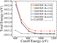
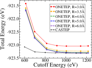
Figure 1: Total energy as calculated by onetep and castep at a fixed geometry as a function of cutoff energy $E_{c}$ and NGWF truncation radius $R_{\phi}$, for the CO₂ molecule (left) and an H₂O dimer (right). Convergence properties are domininated by the oxygen pseudopotential and so are broadly the same for the two systems. The results for 4.0 Å spheres to 6.0 Å spheres agree to high accuracy, particularly at a cutoff energy of 900 eV or above, indicating convergence at around 4.0 Å.

   

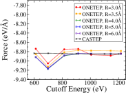
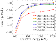
Figure 2: Convergence properties of a single force component calculated using onetep and castep at a fixed, off-equilibrium geometry as a function of cutoff energy $E_{c}$ and NGWF truncation radius $R_{\phi}$, for the CO₂ molecule (left) and an H₂O dimer (right). Force shown is the force acting on an O atom along the bond axis for CO₂, (hence a very strong force), and the force on the hydrogen atom not involved in the dimer-dimer h-bond (hence a very weak force, near-equilibrium). Forces converge with both $R_{\phi}$ and $E_{c}$, but care must be taken to accurately converge with respect to both quantities simultaneously.

We must first investigate the convergence of calculated quantities with respect to the basis size in the two methods. In onetep we can systematically control the convergence by decreasing the grid spacing (which corresponds to a plane-wave cutoff $E_{c}$) and increasing the localisation radii $R_{\phi}$ of the NGWFs. In castep we can vary the plane wave cutoff $E_{c}$. In Fig. 1 we examine the convergence of the total energy of the two molecular systems with respect to these quantities, while in Fig. 2 we examine the convergence of force components. It is observed, as previously noted Skylaris et al. (2005b), that total energy convergence with grid spacing is slower in onetep than in plane-wave methods such castep. This is due to the greater influence of the so-called ‘egg-box’ effect in the former (the variation in energy with uniform translation of the atoms with respect to the grid), which results from NGWF truncation to points within a sphere on a regular underlying grid. However, both methods converge asymptotically to the same value to a high precision. The onetep forces converge non-monotonically with both $E_{c}$ and $R_{\phi}$ to eventual good agreement with the castep equivalents, at a radius not significantly greater than would be required for tolerable convergence of the total energy (around 4.0 Å in this case). It is to be noted that at a fixed, under-converged value of $E_{c}$, convergence with $R_{\phi}$ is to an incorrect value, while at fixed, under-converged $R_{\phi}$, convergence with $E_{c}$ may be erratic or tend to an incorrect value. In particular, very small localisation regions result in highly inaccurate forces. This emphasises the importance of converging with respect to both parameters simultaneously for accurate results. Finally, as with for plane-wave codes, it should be noted that accurate forces will often require higher convergence parameters than accurate energy differences.

To demonstrate that the convergence properties demonstrated here are applicable to larger systems, we examine the difference between the calculated forces in onetep and castep for a larger molecule. We employ the organic zwitterionic detergent molecule, 3-[(3-Cholamidopropyl)dimethylammonio]-1-propanesulfonate, or ‘CHAPS’ as a particularly challenging, worst-case test system, due to the considerable charge separation and long-ranged forces encountered. In Figure 3 we plot the RMS error of all the calculated forces, and observe that they can be systematically converged with respect to local orbital radius and cutoff energy.

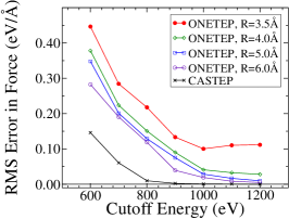
Figure 3: Convergence properties of the RMS error in the onetep and castep forces at a fixed, off-equilibrium geometry as a function of cutoff energy $E_{c}$ and NGWF truncation radius $R_{\phi}$, for the CHAPS molecule (see text). The quantity plotted is the RMS difference between the calculated result for a given $E_{c}$ and $R_{\phi}$ and the calculated result for $E_{c}=1200$eV in castep, which is taken to be the converged result. We see that with respect to both $R_{\phi}$ and $E_{c}$ it is possible to obtain systematic convergence to the plane-wave result.

IV.2 Consistency in molecular systems

We now examine the consistency of the forces and the energy by calculating the full binding curve for the CO₂ molecule and the H₂O molecular dimer. For the castep calculation a plane-wave energy cut-off energy of 1100 eV was used for the wavefunctions, while for onetep a grid-spacing of 0.227 Å (equivalent to a plane-wave energy cut-off of 1121 eV) and four NGWFs on each atom, each with a localisation radius of 4.0 Å, were used. Examination of Figs. 1 and 2 suggest these cutoffs will produce results accurate to within around 10 meV for the total energy and 0.01 eV/Å for the forces in these two systems.

In Fig. 4 the variation of the total energy of a carbon dioxide molecule with respect to the C–O bond length is shown, as calculated with castep (plus symbols) and onetep (open diamonds). The curve drawn is a polynomial fit $E(x)$ to the data points. As can be seen, the results are indistinguishable. The inset to Fig. 4 shows the Hellmann-Feynman force, calculated according to Eq. (7), in castep (plus symbols) and onetep (open diamonds). Again the agreement is excellent. The curve shown in the inset is the analytic derivative $F(x)\equiv-\frac{1}{2}\frac{\mathrm{d}E}{\mathrm{d}x}$ of the polynomial fit to the energy data points. A discrepancy between this curve and the calculated forces would indicate an inconsistency between the PES and the Hellmann-Feynman forces. We see that there is no inconsistency and that any errors introduced by imposing localisation constraints on the NGWFs are negligible. Quantitative comparison of the two approaches shows that the fractional differences in the equilibrium bond length and the curvature of the PES at the minimum, respectively, are less than 0.1% and 0.2%. The discrepancy between the equilibrium bond length as predicted by the numerical force (given by the $x$-intercept of $F(x)$) and by the Hellmann-Feynman force (given by a polynomial fit to the force data points) is less than 0.1% for both approaches.

Figure 4: Total energy as a function of C–O bond-length for a carbon dioxide molecule subjected to a symmetric stretch. castep (plus symbols); onetep (open diamonds). The curve shows a polynomial fit $E(x)$ to the data points. On the scale of this plot the data are indistinguishable. Inset: the Hellmann-Feynman force on each oxygen atom. The curve shows the numerical force $F(x)\equiv-\frac{1}{2}\frac{\mathrm{d}E}{\mathrm{d}x}$.

We turn now to the more challenging case of the water dimer. In Fig. 5 the total energy as a function of the length of the hydrogen bond is shown. This is a much more sensitive test, as the potential well associated with the hydrogen bond is shallower and the forces weaker by two orders of magnitude than in the case of the strong covalent bonds in carbon dioxide.

Figure 5: Interaction potential of a water dimer. castep (plus symbols); onetep (open diamonds). The curves show polynomial fits $E(x)$ to the data points. Inset: the Hellmann-Feynman force on each water molecule. The curves show the numerical force $F(x)\equiv-\frac{\mathrm{d}E}{\mathrm{d}x}$ for castep (dashed line) and onetep (solid line).

For the castep calculation a plane-wave cut-off energy of 1200 eV was used. For onetep, a grid-spacing of 0.214 Å (equivalent to a plane-wave energy cut-off of 1261 eV) was used; each hydrogen and oxygen atom had one and four NGWFs, respectively, all of radius 4.0 Å.

From Fig. 5 it may be seen that the total energies of the two approaches are within 20 meV of each other. The predicted equilibrium bond length and the curvature of the PES at the minimum agree to within 0.3% and 4.6%, respectively, well within the variations associated with using different exchange and correlation functionals. The effect of localisation constraints, however, is now apparent. The inset shows that the Hellmann-Feynman forces in onetep do not coincide perfectly with the derivative of the fit to the total energy. Nevertheless, the discrepancy is small: at the equilibrium bond length the error, defined as the fractional difference between the $x$-intercept of the numerical force (solid line, inset of Fig. 5) and that of a fit (not shown) to the Hellmann-Feynman forces (open diamonds, inset of Fig. 5) is only 0.3%, or 0.005 Å. Note that the forces in onetep agree with the forces in castep even more accurately than the derivative of the fit to the onetep total energy agrees with the corresponding forces. This correlates well with the observed insensitivity of the calculated forces to the effect of truncation of the local orbitals.

IV.3 Convergence and Consistency in Bulk Systems

The above tests for molecules demonstrate the basic applicability of the methods for evaluation of forces within the context of this particular local-orbital method, but do not test their accuracy in the more challenging conditions of a solid, with the constraints necessary for linear-scaling. In particular, in a solid, convergence with local orbital radius can present greater difficulties. To demonstrate the convergence behaviour in solids, we simulate a block of bulk silicon (diamond structure) subject to random distortions of the atomic coordinates about their equilibrium positions and compare the calculated onetep forces on these displaced atoms with those calculated in castep.

We begin with a supercell consisting of $5\times 5\times 5$ times the 8-atom cubic unit cell of the bulk silicon with lattice parameter $a=5.4$ Å, giving 1000 atoms. We then generate a set of realisations of random disorder by displacing each atom according to a uniform random distribution with a given amplitude. These systems are not intended to be physically meaningful apart from as a test of the accuracy of the calculated forces, but are approximately representative of a snapshot of the system at elevated temperature. Calculations were performed with onetep for $R_{\phi}=4.23$ Å, $R_{\phi}=4.76$ Å and $R_{\phi}=5.29$ Å. A fixed psinc spacing of $0.256$ Å corresponding to a plane-wave cutoff of $E_{c}=883$eV, which was verified to give good convergence of both total energies and forces in castep was used in both codes. In the onetep calculations, a kernel cutoff greater than the supercell size was employed, meaning all elements of the density kernel were nonzero, and optimised using the LNV energy minimisation scheme Li et al. (1993). The castep calculations were performed on identical 1000-atom cells with the same plane-wave cutoff. We employed the Local Density Approximation for exchange and correlation. For many systems it is possible to obtain plane-wave accuracy using only as many NGWFs as valence orbitals Skylaris et al. (2005b). However previous onetep calculations on bulk silicon Skylaris and Haynes (2007) have reported that nine NGWFs per silicon atom are required to achieve plane-wave accuracy, and this prescription was followed here.

Table 1 shows the convergence of the forces with respect to the local orbital radius. We see that by $R_{\phi}=4.23$ Å results are already in reasonable agreement with equivalent plane-wave results, with an RMS deviation increasing from 0.001 eV/Å to 0.004 eV/Å as the disorder magnitude $\Delta$ increases. For larger radii the results improve, though the extent to which they can agree with the castep results is limited by the ‘egg-box’ effect resulting from the underlying grid spacing. By $\Delta=0.5a_{0}$, the system is some way off equilibrium, with an RMS force of around 2.3 eV/Å, but the precision of the agreement with plane-wave results is maintained.

$\Delta$ ($a_{0}$)	$R_{\phi}$ ($a_{0}$)	$\phantom{-\mathbf{F}_{\text{CAS}}}|\mathbf{F}|_{\text{max}}$	$|\mathbf{F}-\mathbf{F}_{\text{CAS}}|_{\text{max}}$	$\phantom{-\mathbf{F}_{\text{CAS}}}|\mathbf{F}|_{\text{rms}}$	$|\mathbf{F}-\mathbf{F}_{\text{CAS}}|_{\text{rms}}$
0.00	8.0	0.00135	0.00135	0.00096	0.00096
0.00	9.0	0.00020	0.00020	0.00014	0.00014
0.00	10.0	0.00011	0.00011	0.00008	0.00008
0.05	8.0	0.40748	0.00437	0.22083	0.00193
0.05	9.0	0.40772	0.00357	0.22095	0.00175
0.05	10.0	0.40779	0.00354	0.22091	0.00169
0.50	8.0	6.1615	0.00870	2.22984	0.00414
0.50	9.0	6.1648	0.00450	2.30108	0.00208
0.50	10.0	6.1620	0.00739	2.29999	0.00270

Table 1: Convergence with NGWF radius of atomic forces (eV/Å) for a 1000-atom system of bulk Si subject to random displacements of $\Delta=\{0,0.05,0.5\}a_{0}$, where $a_{0}=0.529$ Å. $\mathbf{F}$ is the force calculated in onetep and $\mathbf{F}_{\text{CAS}}$ its equivalent calculated in castep. Maximum and root mean square forces, plus corresponding values for the maximum and RMS deviation of forces from the castep result are shown for each of $R_{\phi}=\{8,9,10\}a_{0}$. Note that for $\Delta=0$, the castep forces are all zero by symmetry, and the deviation of the onetep results is solely due to the ‘egg-box’ effect and the influence of NGWF truncation.

V Applications

V.1 Si Surface Reconstructions

We now report results of a realistic application of geometry optimisation, using our quasi-Newton scheme, on a Si(001) surface, comparing again with castep. Calculations were performed within the local-density approximation in a 8$\times$8 supercell consisting of nine atomic layers of silicon atoms in which the bottom layer of atoms was hydrogen passivated (a total of 640 atoms). A fixed lattice constant of 5.43 Å was used, resulting in a supercell of dimensions 30.713 Å $\times$ 30.713 Å in the plane of the surface. The size of the supercell in the perpendicular direction was 25.595 Å, providing a vacuum gap of 12.9 Å between adjacent periodic replicas, though this varies slightly during the calculation. For these surface calculations, the same grid spacing of 0.256 Å was used, and localisation radii of 4.0 Å were chosen.

The passivating hydrogen atoms were constrained to lie vertically below the bottom layer of silicon atoms which were fixed to their bulk positions. Surface atoms were given small initial random displacements to break symmetry so that they could dimerise. Symmetry was imposed so that the surface could only form a p(2$\times$1) reconstruction. This allows a direct comparison with a castep calculation on a 2$\times$1 surface supercell comprised of 18 silicon atoms and two passivating hydrogen atoms. A plane-wave cut-off of 883 eV was used for the wavefunctions and the Brillouin zone was sampled using an evenly spaced grid consisting of 4$\times$8 k-points in castep. The same pseudopotentials were used for both onetep and castep calculations.

Figure 6: Schematic of the reconstructed Si(001) surface. Bonds indicated by dashed lines do not lie in the plane of the diagram. The surface atoms (indicated by white circles) pair up to form dimers, that then buckle out of the plane of the surface. For the purposes of this work the bonds have been labelled alphabetically and the buckling angle denoted by $\theta$.

	A	B	C	D	E	F	G	$\theta$
onetep	2.306	2.272	2.364	2.362	2.398	2.333	2.364	17.9∘
castep	2.313	2.274	2.371	2.378	2.403	2.338	2.380	17.0∘
Ref Ramstad et al. (1995).	2.29	2.26	2.34	2.35	2.38	2.33	2.35	18.3∘

Table 2: Bond lengths (in Angstrom) and the buckling angle $\theta$ as calculated by onetep, castep and Ramstad et al. Ramstad et al. (1995).

As expected surface atoms were observed to pair up to form dimers, which then buckled out of the plane of the surface. The resulting geometry is shown in Fig. 6. Bond lengths and buckling angles are compared in Table 2. They compare very well with all bond lengths lying within 0.02 Å. The differences in bond lengths lead to a slightly smaller buckling angle in castep compared to onetep. The bond lengths also compare well with those found in previous work by Ramstad et. al. Ramstad et al. (1995). The shorter bond lengths found in that work can be attributed to the use of different pseudopotentials.

Regarding the number of NGWFs/atom, we observed here that using only four NGWFs per silicon, surface atoms did dimerise but the resulting dimers failed to buckle. The flexibility afforded by nine NGWFs appears to be required for the dimers to relax into the buckled geometry.

V.2 Charge Redistribution

Finally we report on geometry convergence tests for structural optimisation in more complex systems exhibiting charge redistribution, to test the performance of the algorithms. System (a) is the CHAPS molecule referred to in Sec. IV.1. Its zwitterionic nature leads to considerable charge separation and some relatively long-ranged contributions to the forces, hence a challenging case for geometry relaxation. We started from standard crystallographic data Kleywegt and Jones (1998), with hydrogen atoms added to saturate dangling bonds. The resulting molecule contains 100 atoms. System (b) is a crystalline ceramic of 119 atoms, comprising a $2\times 2\times 1$ supercell of $\alpha-$alumina in the corundum structure, containing one aluminium vacancy $\mathrm{V}_{\mathrm{Al}}^{-3}$ in charge state $-3$ (such that neighbouring oxygens retain filled $p$-shells). The starting configuration used for the relaxation was the optimised bulk geometry before removal of the aluminium atom. In this ionic system, containing a vacancy with a large net charge, there are again considerable long-ranged relaxations. Finally, system (c) is a small nanocrystal of wurtize-structure GaAs, a polar semiconductor. Starting from the bulk wurtzite crystal structure optimised within DFT, the nanocrystal is imagined to have been formed by cleaving to expose [0001] faces on the two ends, corresponding to Ga and As layers, respectively. There remains a net dipole moment parallel to the $c$-axis, whose value depends on the geometry of the surfaces. The rod, comprising 204 atoms once dangling bonds are terminated with hydrogen, was simulated inside a cubic simulation cell of side-length 45 Å. These systems are illustrated in Fig. 7.

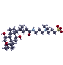
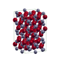
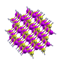
Figure 7: Systems for which geometry optimisation was performed with the BFGS algorithm in onetep for illustration of convergence behaviour. Left: CHAPS molecule (100 atoms) Centre: Al vacancy in $2\times 2\times 1$ supercell of $\alpha-$alumina (119 atoms) Right: H-terminated GaAs nanocrystal (204 atoms)

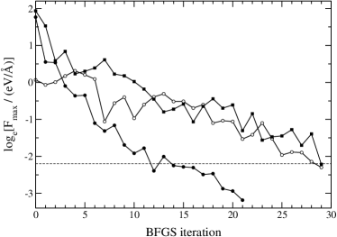
Figure 8: Convergence behaviour of the maximum force $|F_{\mathrm{max}}|$ on any atom as the BFGS algorithm proceeds for the typical systems shown in Fig. 7. CHAPS Zwitterion (open circles); Al vacancy in alumina (filled circles); GaAs nanocrystal (squares). Dashed line shows convergence threshold of 0.11 eV/Å. Simultaneous convergence of total energy and the maximum displacement were required, with $|\mathrm{d}\mathbf{R}_{\mathrm{max}}|=0.002$ Å  for 2 successive iterations was also required. From the starting coordinates (see text) convergence was achieved in 29, 21 and 29 iterations respectively.

Fig. 8 shows the convergence behaviour of the maximum force as the BFGS algorithm progresses in each case. In all three cases, convergence is achieved after 20-30 iterations. The forces agree to good precision with those obtained in comparable calculations in castep, so the optimisations follow a similar path. The demands of convergence tolerance on plane-wave cut-off and sizes of the localisation regions are not significantly greater than those required for accurate evaluation of the energy in these systems. As with plane-wave calculations, tight convergence of the electronic energy is required before the forces are well-converged, since the error in the forces scales approximately as the square root of the error in the energy. We therefore conclude that it is possible to perform geometry optimisation in the current framework with a similar relative performance overhead compared to single-point energies as in plane-wave DFT.

V.3 Scaling with System Size

Finally, we demonstrate the scaling of the timings of the evaluation of the forces compared to the total energy minimisation. As we have described, the efficient parallel algorithms used ensure that despite the $O(N^{2})$ prefactor on parts of the force calculation, the total computational time remains dominated by optimisation of the NGWFs and density kernel at each BFGS trial step up to very large $N$. We show in Fig. 9 the total time taken by various parts of the calculation for a series of systems each comprising double helices of DNA of increasing length (with randomly chosen base pair sequences to ensure no advantage can be gained through periodicity). The base-pair sequences were generated randomly, and the atom positions created with the Nucleic Acid Builder Macke and Case (1998) code. The positions were relaxed within an empirical potential framework, using the Amber code Case et al. (2010). This generated a starting point where the forces on the atoms were low but non-zero, since the empirical-potential forces do not exactly match those from the (presumably more accurate) DFT calculation.

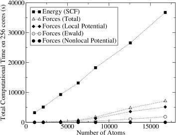
Figure 9: Scaling of total computational time for SCF total energy calculation for a series of DNA molecules of increasing length (squares), compared to scaling of total computational time for forces calculation (triangles), and the three force components present: Ewald, Local Potential and Nonlocal Potential (diamonds, empty circles and filled circles respectively), for the same simulations.

This system has previously been shown to exhibit good linear-scaling with number of atoms $N$, and scale well to large numbers of processorsHine et al. (2010). The calculations here were performed with a plane-wave energy cut-off of 700 eV, localisation radii 3.7 Å, and a density kernel cutoff radius of 16 Å. These are somewhat lower accuracy values than used in the previous tests, so as to allow scaling to very large system sizes within moderate memory requirements, but should still allow for reasonable convergence of the forces according to the findings in Sec IV.1. Note that in DNA, with a very small HOMO-LUMO gap, the density matrix is quite long-ranged and a relatively large cutoff must be used.

We report in Fig. 9 timings for a total energy minimisation followed by a calculation of the forces on 256 parallel cores (Intel COREi7 CPUs). We vary the size of the system from 1042 atoms (16 base pairs) up to 16775 atoms (256 base pairs), scaling the unit cell commensurately along one direction. Note that even the smallest of these systems would be beyond the feasible scope of conventional PWP methods, given the size of the simulation cell. The total time for the optimisation of the electronic degrees of freedom is seen to scale nearly perfectly as $O(N)$, while the calculation of the local pseudopotential forces scales as roughly $O(N^{2})$ (though the improved computational load balance at large system sizes masks this slightly). Consequently, the fraction of the total time accounted for by the forces increases from under 1% to nearly 20%. Eventually, the calculation of forces would dominate and the method could no longer be termed linear-scaling. However, this is not expected to be the case in typical systems such as the DNA strands shown here until upwards of 30000 atoms. Of course, this does not imply that a fully converged geometry optimisation would be necessarily possible in linear-scaling computational effort. An additional problem is the fact that ionic relaxation requires a number of iterations, or evaluations of the potential energy surface (PES), that increases with the number of atomsGoedecker et al. (2001). Preliminary steps have been taken by other authors Goedecker et al. (2001); Fernández-Serra et al. (2003); Nemeth and Challacombe (2004, 2005) towards addressing this issue in the context of large-scale calculations. This is outside the scope of the present work, however; often in practice it will be sufficient to relax a smaller sub-region of a very large system, thereby making the optimisation procedure tractable, or one might in any case be investigating the effect of a localised perturbation to an otherwise relaxed system. In such cases, we have shown that geometry optimisation with plane-wave accuracy and linear-scaling computational effort is achievable up to tens of thousands of atoms.

VI Conclusions

In conclusion, we have shown that the combination of using strictly-localised non-orthogonal generalised Wannier functions that move with the ions but that are optimised on-the-fly within a basis set of psinc functions that are fixed with respect to the ions, within the onetep linear scaling DFT method, results in potential energy surfaces that are sufficiently smooth that ionic forces can be calculated with high accuracy. We have demonstrated that these forces can be systematically converged with respect to energy cutoff and local orbital radius to high-precision with low overhead relative to the demands of a comparable total energy calculation. We have demonstrated this by performing geometry optimisation on a set of widely varied systems and comparing to calculations using conventional plane-wave DFT. We note that for weaker bonds, such as hydrogen bonds, although the discrepancy between the PES and the calculated forces becomes more noticeable (Fig. 5), the effect is nonetheless very small. Finally, we have demonstrated that geometry optimisation is possible with a comparable computational overhead to that for PWP simulations, and that the forces calculation, while scaling as $\mathcal{O}(N^{2})$, remains a small fraction of the total computational time until upwards of 30000 atoms for typical systems.