Electron-electron scattering and nonequilibrium noise in Sharvin contacts

Abstract

We consider wide ballistic microcontacts with electron-electron scattering in the leads and calculate electric noise and nonlinear conductance in them. Due to a restricted geometry the collisions of electrons result in a shot noise even though they conserve the total momentum of electrons. We obtain the noise and the conductivity for arbitrary relations between voltage $V$ and temperature $T$. The positive inelastic correction to the Sharvin conductance is proportional to $T$ at low voltages $eV\ll T$, and to $|V|$ at high voltages. At low voltages the noise is defined by the Nyquist relation and at high voltages the noise is related with the inelastic correction to the current by the Shottky formula $S_{in}=2e\,I_{in}$.

Nonequilibrium electric noise is observed in most mesoscopic systems. It depends on the conduction mechanism and is more sensitive to the effects of electron-electron interactions than the average conductance  Blanter99 . In this article we are concerned with Sharvin-type ballistic contacts. In the absence of scattering near the contact, all the relaxation processes that lead to dissipation and a finite resistance of the contact take place deep in the leads, where the electron distribution is almost equilibrium. As the motion of electrons in the nonequilibrium region near the contact is purely deterministic, the noise does not depend on the voltage and is specified by the Nyquist relation involving the equilibrium Sharvin conductance. If any impurities are present in the contact, this results in a positive contribution to the resistance and in a shot noise, which is proportional to the current. Unlike the impurity scattering, electron-electron collisions do not contribute to the resistivity of a homogeneous conductor with a parabolic spectrum because they conserve the total momentum of electrons. However very recently, it was shown both experimentally Renard08 and theoretically Nagaev08 that electron–electron scattering may result in a negative correction to the resistance of wide ballistic contacts. Therefore it is of interest to calculate the voltage-dependent electric noise in them and to find out whether collisions of electrons result in a shot noise like impurity scattering.

Effects of electron-electron interaction on the shot noise have been extensively studied in the past for contacts with imperfect transmission. More than a decade ago, they were considered semiclassically for diffusive multichannel microbridges Nagaev95 . More recently, a number of authors considered interaction effects in the shot noise of microstructures by modeling them as conducting quantum dots that were either in the Kondo Mora08 ; Gogolin06 or Coulomb-blockade Loss00 ; Bagrets05 regime. The interaction was assumed to take place between electrons in localized states on these dots. Naturally, this interaction strongly differs from that in the bulk of the conductor. However our recent results show that even collisions of electrons far from the contact affect the average current and hence may cause its fluctuations.

To calculate the noise, we use the semiclassical Boltzmann-Langevin method Kogan . Previously, Kulik and Omelyanchuk used a similar approach to calculate electric noise in Sharvin contacts caused by electron-phonon scattering in the zero-temperature limit Kulik84 . Here we extend this approach to arbitrary temperatures.

We adopt a model of a ballistic contact similar to that of Kulik et al. Kulik77 for the case of electron–phonon scattering. Consider two 2D electron gases separated by a thin impenetrable barrier with a gap of width $2a$. We assume that $a$ is much larger than the Fermi wavelength and the screening radius but much smaller than both elastic and inelastic mean free path of electrons. The distribution functions of electrons on both sides of the insulator obey the Boltzmann equation

$$\frac{\partial f}{\partial t}+{\bf v}\,\frac{\partial f}{\partial{\bf r}}+e{\bf E}\,\frac{\partial f}{\partial{\bf p}}=\hat{I}_{ee},$$ (1)

where ${\bf E}=-\nabla\varphi$ is the electric field. The electron–electron collision integral in this equation is given by

$$I_{ee}=\frac{1}{2}\sum_{{\bf p}^{\prime}{\bf k}{\bf k}^{\prime}}\Bigl{[}J({\bf p}^{\prime}{\bf k}^{\prime}\to{\bf p}{\bf k})-J({\bf p}{\bf k}\to{\bf p}^{\prime}{\bf k}^{\prime})\Bigr{]},$$ (2)

where

$$J({\bf p}{\bf k}\to{\bf p}^{\prime}{\bf k}^{\prime})=W({\bf p}{\bf k}|{\bf p}^{\prime}{\bf k}^{\prime})\,f({\bf p})\,f({\bf k})$$

$$\times[1-f({\bf p}^{\prime})]\,[1-f({\bf k}^{\prime})]$$ (3)

and $W({\bf p}{\bf k}|{\bf p}^{\prime}{\bf k}^{\prime})=8\pi^{2}\alpha_{ee}\nu^{-2}\,V_{vol}^{-3}\,\delta(\varepsilon_{{\bf p}}+\varepsilon_{{\bf k}}-\varepsilon_{{\bf p}^{\prime}}-\varepsilon_{{\bf k}^{\prime}})\,\delta({\bf p}+{\bf k}-{\bf p}^{\prime}-{\bf k}^{\prime})$ is the probability of a transition from the state $({\bf p},{\bf k})$ to the state $({\bf p}^{\prime},{\bf k}^{\prime})$. Here $\alpha_{ee}$ is a dimensionless parameter of electron-electron scattering and $\nu=m/\pi$ is the two-dimensional density of states. Equation (1) should be solved together with the Poisson equation for the electric potential $\varphi$. It is possible to avoid solving the latter using the condition $E_{F}\gg{\rm max}(eV,T)$ Kulik84 , which means that in the absence of collisions, electrons near the Fermi surface just move along straight lines. This condition allows us to set ${\bf v}=v_{F}{\bf p}/p$ and remove the term with electric field from Eq. (1).

Now we should specify the boundary conditions to calculate the distribution functions using Eq. (1). We set $f({\bf p})=f_{0}(\varepsilon_{{\bf p}})$ and $\varphi=\pm V/2$ far from the gap in the left and right half-planes.

If collisions are neglected, $f({\bf p},{\bf r})$ depends solely on whether the electron trajectory originates from gap or not. It is convenient to use a notion of the angular domain $\Omega_{in}({\bf r})$ that contains all the momenta of electrons that came to point ${\bf r}$ from the contact. In terms of this domain, the zero approximation distribution function is

$$f^{(0)}_{L,R}({\bf p},{\bf r})=\left\{\begin{array}[]{ll}f_{0}(\varepsilon_{{\bf p}}+e\varphi({\bf r})\mp eV/2),&{\bf p}\notin\Omega_{in}({\bf r})\\ f_{0}(\varepsilon_{{\bf p}}+e\varphi({\bf r})\pm eV/2),&{\bf p}\in\Omega_{in}({\bf r})\end{array}\right.$$ (6)

for the electrons in left (upper sign) and right (lower sign) half-spaces, respectively.

The current through the contact is given by

$$I=e\int\limits_{-a}^{a}{d\rho\int{\frac{d^{2}p}{(2\pi)^{2}}v_{\perp}f({\bf p},{\bm{\rho}})}}.$$ (7)

where $v_{\perp}$ is the component of $\bf{v}$ normal to the insulator and vector ${\bm{\rho}}=\bf{e}_{\parallel}\rho$ labels points within the gap in the plane of insulator. Substituting expressions (6) into Eq. (7) results in the well known expression for the Sharvin conductance $G_{0}=e^{2}p_{F}a/\pi^{2}$. The first-order correction in scattering to $G_{0}$ can be calculated by substituting $f({\bf p},{\bf r})$ from Eq. (1) into Eq. (7)

$$I_{in}=e\int\limits_{-a}^{a}d\rho\int\frac{d^{2}p}{(2\pi)^{2}}\,v_{\perp}\int\limits_{0}^{\infty}d\tau\,I_{ee}\{f^{(0)}({\bf p}(\tau),{\bf r}(\tau))\}.$$ (8)

Here $\tau$ is the time of travel to point $\bm{\rho}$ along the trajectory.

The collision integral (2) involves four electron momenta ${\bf p}$, ${\bf k}$, ${\bf p}^{\prime}$, and ${\bf k}^{\prime}$. If none of electrons with these momenta crosses the gap (i.e. falls within $\Omega_{in}({\bf r})$), a substitution of distribution functions (6) into (2) results in $I_{ee}=0$. As it was shown in Refs. Nagaev08 and Nagaev09 , the main contribution to the current (8) comes from collisions at points ${\bf r}$ located much farther from the gap than its size $a$. Hence $\Omega_{in}({\bf r})$ may be considered as small and the fewer of the four momenta are in $\Omega_{in}({\bf r})$, the larger the contribution to the current. Also in Refs. Nagaev08 and Nagaev09 it was shown that the largest contribution to the current comes from the collisions of electrons incident on the gap with electrons that are injected from the other half plane and have nearly opposite momentum. Therefore we can assume that only the electrons with momentum ${\bf k}$ are injected and lie in $\Omega_{in}({\bf r})$ while the electrons with the rest of momenta ${\bf p}$, ${\bf p}^{\prime}$, and ${\bf k}^{\prime}$ are native to the considered half-plane.

We sequentially integrate in Eq. (8) over the time, coordinate and momenta as it was done in Ref. Nagaev09 for the case of low voltage $eV\ll T$. Here we consider the case of arbitrary voltages and obtain the correction to the current in a form of an integral over the energies

$$I_{in}=\frac{ea^{2}\alpha_{ee}m}{2(2\pi)^{3}}\ln\frac{l_{c}}{a}\int{d\varepsilon_{{\bf p}}}\int{d\varepsilon_{{\bf k}}}\int{d\varepsilon_{{\bf p}^{\prime}}}\int{d\varepsilon_{{\bf k}^{\prime}}}\\ \times F_{0}(\varepsilon_{{\bf p}},\varepsilon_{{\bf k}},\varepsilon_{{\bf p}^{\prime}},\varepsilon_{{\bf k}^{\prime}})\,\delta(\varepsilon_{{\bf p}}+\varepsilon_{{\bf k}}-\varepsilon_{{\bf p}^{\prime}}-\varepsilon_{{\bf k}^{\prime}})\\ \times\Theta(D)/\sqrt{D},$$ (9)

where $l_{c}$ is a cutoff length much larger than $2a$, which may be due to a very weak electron-impurity scattering or a finite size of the electrodes,

$$F_{0}(\varepsilon_{{\bf p}},\varepsilon_{{\bf k}},\varepsilon_{{\bf p}^{\prime}},\varepsilon_{{\bf k}^{\prime}})\\ =[1-f_{L}(\varepsilon_{{\bf p}})]\,[1-f_{R}(\varepsilon_{{\bf k}})]\,f_{L}(\varepsilon_{{\bf p}^{\prime}})\,f_{L}(\varepsilon_{{\bf k}^{\prime}})\\ {}-f_{L}(\varepsilon_{{\bf p}})\,f_{R}(\varepsilon_{{\bf k}})\,[1-f_{L}(\varepsilon_{{\bf p}^{\prime}})]\,[1-f_{L}(\varepsilon_{{\bf k}^{\prime}})],$$ (10)

and

$$D=\left[(\varepsilon_{{\bf p}}-\varepsilon_{{\bf k}})^{2}-(\varepsilon_{{\bf p}^{\prime}}-\varepsilon_{{\bf k}^{\prime}})^{2}\right]/4$$ (11)

is a value characterizing the deviation of the energies from the Fermi surface, which vanishes when all the energies lie exactly at the Fermi surface. This expression allows us to analytically obtain the results in the limiting cases of high and low voltages and numerically calculate the correction for arbitrary relations $eV/T$. At high voltages $eV/T\gg 1$ the correction to the current has a form

$$I_{in}=\frac{ea^{2}\alpha_{ee}m}{(2\pi)^{3}}\,\ln\frac{l_{c}}{a}\times\left(1-\frac{\pi}{4}\right){\rm sign}(V)(eV)^{2}$$ (12)

and at low voltages $eV/T\ll 1$

$$I_{in}=\frac{ea^{2}\alpha_{ee}m}{(2\pi)^{3}}\ln\frac{l_{c}}{a}\times\frac{C_{10}}{2}(eV)T$$ (13)

where the constant $C_{10}=3.72$.

Using the above semiclassical model, we can calculate the noise spectral density. It is expressed through the Fourier transform of the current correlation function as follows

$$S=2\int\limits_{-\infty}^{\infty}{dt\,e^{i\omega t}\langle\delta I(t)\,\delta I(0)\rangle}.$$ (14)

We will calculate the spectral density at zero frequency $\omega=0$. Current fluctuation can be expressed in terms of fluctuation of the distribution function by the Eq. (7), so the current correlator has a form

$$\langle\delta I(t)\,\delta I(0)\rangle=e^{2}\int\limits_{-a}^{a}{d\rho_{1}}\int\limits_{-a}^{a}{d\rho_{2}}\int{\frac{d^{2}p_{1}}{(2\pi)^{2}}}\int{\frac{d^{2}p_{2}}{(2\pi)^{2}}}\\ \times v_{1\perp}v_{2\perp}\,\langle\delta f({\bf p}_{1},{\bm{\rho}_{1}},t)\,\delta f({\bf p}_{2},{\bm{\rho}_{2}},0)\rangle.$$ (15)

The fluctuation $\delta f({\bf p},{\bf r},t)$ obeys the Boltzmann-Langevin equation Kogan

$$\left(\frac{\partial}{\partial t}+{\bf v}\frac{\partial}{\partial{\bf r}}+e{\bf E}\frac{\partial}{\partial{\bf p}}\right) \delta f({\bf p},{\bf r},t)+\frac{\partial f}{\partial{\bf p}}\,e\delta{\bf E}$$

$$=\delta I_{ee}({\bf p},{\bf r},t)+ \delta J^{ext}({\bf p},{\bf r},t),$$ (16)

where $\delta J^{ext}({\bf p},{\bf r},t)$ is a Langevin source. The correlator of Langevin sources was calculated in Kogan69 on the assumption that each collision is correlated only with itself and equals

$$\langle\delta J^{ext}({{\bf r}_{1}},t_{1},{\bf p}_{1})\,\delta J^{ext}({{\bf r}_{2}},t_{2},{\bf p}_{2})\rangle=\frac{1}{2}\,V_{vol}\,\delta({\bf r}_{1}-{\bf r}_{2})\\ \times\delta(t_{1}-t_{2})\biggl{[}\delta_{{\bf p}_{1}{\bf p}_{2}}\sum\limits_{{\bf p}^{\prime}{\bf k}{\bf k}^{\prime}}(J_{{\bf p}^{\prime}{\bf k}^{\prime}\to{\bf p}_{1}{\bf k}}+J_{{\bf p}_{1}{\bf k}\to{\bf p}^{\prime}{\bf k}^{\prime}})\\ {}+\sum\limits_{{\bf p}^{\prime}{\bf k}^{\prime}}(J_{{\bf p}^{\prime}{\bf k}^{\prime}\to{\bf p}_{1}{\bf p}_{2}}+J_{{\bf p}_{1}{\bf p}_{2}\to{\bf p}^{\prime}{\bf k}^{\prime}})\\ {}-2\sum\limits_{{\bf k}{\bf k}^{\prime}}(J_{{\bf p}_{1}{\bf k}\to{\bf k}^{\prime}{\bf p}_{2}}+J_{{\bf k}^{\prime}{\bf p}_{2}\to{\bf p}_{1}{\bf k}})\biggr{]}$$ (17)

We can neglect the field terms in (16) for the same reason as it was done for the Boltzmann equation (1). As we consider finite temperatures, we have to take into account equilibrium fluctuations of $f$ far from contact. To this end, we present $\delta f$ as a sum of fluctuation $\delta f_{0}$ that has arrived from the depth of electrode by freely propagating without scattering Kulik' and the integral of the right-hand side of Eq. (16) over time $\tau$ of travel to point ${\bf r}$ along the trajectory of a free electron

$$\delta f({\bf p},{\bf r},t) =\delta f_{0}({\bf p},{\bf r},t)+\int\limits_{0}^{\infty}{d\tau}\left[\delta I_{ee}({\bf p},{\bf r}-{\bf v}\tau,t-\tau)\right.$$

$${}+ \left.\delta J^{ext}({\bf p},{\bf r}-{\bf v}\tau,t-\tau)\right].$$ (18)

Therefore the correlator of distribution functions in Eq. (15) is given by

$$\langle\delta f({\bf p}_{1},{\bm{\rho}_{1}},t)\,\delta f({\bf p}_{2},{\bm{\rho}_{2}},0)\rangle\\ =\langle\delta f_{0}({\bf p}_{1},{\bm{\rho}_{1}},t)\,\delta f_{0}({\bf p}_{2},{\bm{\rho}_{2}},0)\rangle\\ {}+\int\limits_{0}^{\infty}{d\tau}\Bigl{[}\langle\delta f_{0}({\bf p}_{1},{\bm{\rho}_{1}},t)\,\delta I_{ee}({\bf p}_{2},\rho_{2}-{\bf v_{2}}\tau,-\tau)\rangle\\ {}+\langle\delta f_{0}({\bf p}_{2},{\bm{\rho}_{2}},0)\,\delta I_{ee}({\bf p}_{1},\rho_{1}-{\bf v_{1}}\tau,t-\tau)\rangle\Bigr{]}\\ {}+\int\limits_{0}^{\infty}{d\tau_{1}}\int\limits_{0}^{\infty}{d\tau_{2}}\,\langle\delta J^{ext}({\bf p}_{1},{\bm{\rho}_{1}}-{\bf v_{1}}\tau_{1},t-\tau_{1})\\ {}\times\delta J^{ext}({\bf p}_{2},{\bm{\rho}_{2}}-{\bf v_{2}}\tau_{2},-\tau_{2})\rangle.$$ (19)

Note that $\delta f_{0}$ and $\delta J^{ext}$ are totally uncorrelated because of the causality principle. The first term in (17) is the two-time correlation function of fluctuations that originate from the depth of electrodes and propagate to the point of observation without scattering. This correlation function is well known deJong96

$$\langle\delta f_{0} ({\bf p}_{1},{\bm{\rho}_{1}},t)\delta f_{0}({\bf p}_{2},{\bm{\rho}_{2}},0)\rangle=(2\pi)^{2}\,\delta({\bf p}_{1}-{\bf p}_{2})$$

$$\times \delta({\bm{\rho}_{1}}-{\bm{\rho}_{2}}-{\bf v_{1}}t)\,f({\bf p}_{1})[1-f({\bf p}_{1})].$$ (20)

Substituting this correlator to (15) and (14) results in the Nyquist equation $S_{0}=4TG_{0}$, where $G_{0}$ is the Sharvin conductance.

To the first order in the scattering, the spectral density $S_{in}=S-S_{0}$ is defined by the last three summands in Eq. (19). In the second and the third summands of this equation, $\delta I_{ee}$ is obtained by variating the collision integral $I_{ee}$ (2) with respect to $\delta f$. To obtain the results to the first order in the interaction, we substitute the distribution functions (6) in $\delta I_{ee}$ and evaluate the correlators $\langle\delta f_{0}\,\delta I_{ee}\{\delta f\}\rangle$ and $\langle\delta I_{ee}\{\delta f\}\,\delta f_{0}\rangle$ using the zero-approximation correlators Eq. (20). The fourth summand in Eq. (19) is obtained directly from Eq. (17). Then we substitute the resulting expressions into Eqs. (15) and (14).

After some rearrangements the first-order spectral density takes up a form

$$S_{in}=2e^{2}V_{vol}\int\limits_{0}^{\infty}{dt}\int\limits_{-a}^{a}{d\rho_{1}}\int\limits_{-a}^{a}{d\rho_{2}}\int{\frac{d^{2}p_{1}}{(2\pi)^{2}}}\int{\frac{d^{2}p_{2}}{(2\pi)^{2}}}\\ {}\times v_{1\perp}v_{2\perp}\int\limits_{0}^{\infty}\!{d\tau_{1}}\int\limits_{0}^{\infty}\!d\tau_{2}\,\delta({\bm{\rho}_{1}}-{\bm{\rho}_{2}}+{\bf v_{2}}\tau_{1}-{\bf v_{1}}\tau_{1}-{\bf v_{2}}t)\\ {}\times\!\!\left.\Bigl{[}\delta(t-\tau_{1}-\tau_{2})\,\Gamma_{1}+\delta(t-\tau_{1}+\tau_{2})\,\Gamma_{2}\Bigr{]}\right|_{\bm{\rho}_{1}-{\bf v}_{1}\tau_{1}},$$ (21)

where $\Gamma_{1}$ and $\Gamma_{2}$ are combinations of distribution functions and scattering fluxes

$$\Gamma_{1}=-\sum\limits_{{\bf p}^{\prime}{\bf k}^{\prime}}\Bigl{\{}f({\bf p}_{2})\,J_{{\bf p}^{\prime}{\bf k}^{\prime}\to{\bf p}_{1}{\bf p}_{2}}\\ +[1-f({\bf p}_{2})]\,J_{{\bf p}_{1}{\bf p}_{2}\to{\bf p}^{\prime}{\bf k}^{\prime}}\Bigr{\}}+2\sum\limits_{{\bf k}{\bf k}^{\prime}}\Bigl{\{}f({\bf p}_{2})\,J_{{\bf p}_{1}{\bf k}\to{\bf p}_{2}{\bf k}^{\prime}}\\ +[1-f({\bf p}_{2})]\,J_{{\bf p}_{2}{\bf k}^{\prime}\to{\bf p}_{1}{\bf k}}\Bigr{\}},$$ (22)

$$\Gamma_{2}=\delta_{{\bf p}_{1}{\bf p}_{2}}[1-2f({\bf p}_{1})]\!\sum\limits_{{\bf p}^{\prime}{\bf k}{\bf k}^{\prime}}(J_{{\bf p}^{\prime}{\bf k}^{\prime}\to{\bf p}_{2}{\bf k}}-J_{{\bf p}_{2}{\bf k}\to{\bf p}^{\prime}{\bf k}^{\prime}})\\ {}+[1-f({\bf p}_{1})-f({\bf p}_{2})]\sum\limits_{{\bf p}^{\prime}{\bf k}^{\prime}}(J_{{\bf p}^{\prime}{\bf k}^{\prime}\to{\bf p}_{1}{\bf p}_{2}}-J_{{\bf p}_{1}{\bf p}_{2}\to{\bf p}^{\prime}{\bf k}^{\prime}})\\ {}+2\,[f({\bf p}_{2})-f({\bf p}_{1})]\sum\limits_{{\bf k}{\bf k}^{\prime}}(J_{{\bf p}_{1}{\bf k}\to{\bf p}_{2}{\bf k}^{\prime}}-J_{{\bf p}_{2}{\bf k}^{\prime}\to{\bf p}_{1}{\bf k}}).$$ (23)

The two terms in Eq. (21) have different physical meaning. The first of them corresponds to the case where the collision takes place during the time interval between the two crossings of the gap by the participating electrons (Fig. 1a). It originates from the collision integral in Eq. (16) and determines the Nyquist noise at $V=0$. This term vanishes at $T=0$ for any $V$ because it results from the equilibrium fluctuations in the depth of electrodes. The second term corresponds to the case where both electrons cross the gap after the collision (Fig. 1b) and results from the corrections to the one-time correlation function of $\delta f$. In equilibrium this function is a thermodynamic quantity and does not depend on the strength of scattering. Therefore the scattering corrections to it and the second term in Eq. (21) vanish at $V=0$.

Consider now (21) and isolate the dominant terms in it. To give a contribution to $\delta I$’s, both the momenta ${\bf p}_{1}$ and ${\bf p}_{2}$ must lie either in the angular domain $\Omega_{in}$ or in the centrally symmetric domain $\Omega_{out}$ (see Fig. 1, inset). As well as for the correction to the current, the contribution to the spectral density of noise is dominated by electron collisions far from the contact, so the angular domains are small and the contribution to the noise is maximum if a minimally possible number of electron momenta involved in scattering is restricted to $\Omega_{in}$ or $\Omega_{out}$. On the other hand, the colliding electrons must have almost opposite momenta to ensure maximum phase space available for the scattering.

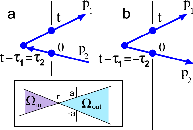
Figure 1: Fig. 1. Illustration of the two terms in Eq. (21). An electron with momentum ${\bf p}_{1}$ crosses the gap at time $t>0$. Another electron with momentum ${\bf p}_{2}$ crosses the gap at time $0$. The collision takes place at $t-\tau_{1}<t$. (a) The first term corresponds to the collision of electrons between the crossing of the gap; $\tau_{2}$ is the time between the first crossing and the collision. (b) The second term corresponds to the collision before both crossings; $\tau_{2}$ is the time between the collision and the first crossing. The inset shows the domains $\Omega_{in}({\bf r})$ and $\Omega_{out}({\bf r})$.

In the first term with $\delta(t-\tau_{1}-\tau_{2})$, momenta ${\bf p}_{1}$ and ${\bf p}_{2}$ have opposite directions (see Fig. 1a) and lie in $\Omega_{out}$ and $\Omega_{in}$, respectively. To ensure maximum phase space for the scattering, ${\bf p}_{1}$ and ${\bf p}_{2}$ must correspond either to the two initial or the two final states. Hence only the first sum should be retained in Eq. (22).

In the second term with $\delta(t-\tau_{1}+\tau_{2})$, momenta ${\bf p}_{1}$ and ${\bf p}_{2}$ are both in $\Omega_{out}({\bf r})$ (see Fig. 1b) and cannot have opposite momenta. To make Eq. (23) nonzero, the electron with ${\bf k}$ must be in $\Omega_{in}({\bf r})$. Hence the dominant contribution to Eq. (23) arises from the first term because $\delta_{{\bf p}_{1}{\bf p}_{2}}$ in it lifts one of the three restrictions on the momentum integration.

We substitute the corresponding terms of Eqs. (22) and (23) into Eq. (21), sequentially integrate over times, momenta and coordinates and obtain the spectral density in a form of an integral over energies

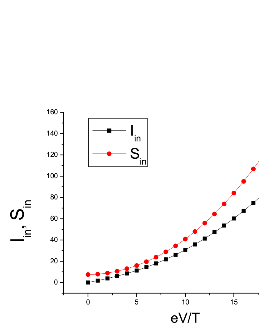
Figure 2: Fig. 2. Dependencies of corrections to the current, measured in $ea^{2}\alpha_{ee}m/(2\pi)^{3}$, and spectral density, measured in $e^{2}a^{2}\alpha_{ee}m/(2\pi)^{3}$, on $eV/T$.

$$S_{in}=\frac{e^{2}a^{2}\alpha_{ee}m}{(2\pi)^{3}}\ln\frac{l_{c}}{a}\int{d\varepsilon_{{\bf p}}}\int{d\varepsilon_{{\bf k}}}\int{d\varepsilon_{{\bf p}^{\prime}}}\int{d\varepsilon_{{\bf k}^{\prime}}}\\ \times\delta(\varepsilon_{{\bf p}}+\varepsilon_{{\bf k}}-\varepsilon_{{\bf p}^{\prime}}-\varepsilon_{{\bf k}^{\prime}})\,\Theta(D)\,D^{-1/2}\\ \times\bigl{[}F_{1}(\varepsilon_{{\bf p}},\varepsilon_{{\bf k}},\varepsilon_{{\bf p}^{\prime}},\varepsilon_{{\bf k}^{\prime}})+F_{2}(\varepsilon_{{\bf p}},\varepsilon_{{\bf k}},\varepsilon_{{\bf p}^{\prime}},\varepsilon_{{\bf k}^{\prime}})\bigr{]},$$ (24)

where

$$F_{1}=2f_{R}(\varepsilon_{{\bf k}})[1-f_{R}(\varepsilon_{{\bf k}})]\Bigl{\{}[1-f_{L}(\varepsilon_{{\bf p}})]\,f_{L}(\varepsilon_{{\bf p}^{\prime}})f_{L}(\varepsilon_{{\bf k}^{\prime}})\\ {}+f_{L}(\varepsilon_{{\bf p}})[1-f_{L}(\varepsilon_{{\bf p}^{\prime}})][1-f_{L}(\varepsilon_{{\bf k}^{\prime}})]\Bigr{\}}$$ (25)

and

$$F_{2}=[1-2f_{L}(\varepsilon_{{\bf p}})]F_{0}$$ (26)

with $F_{0}$ defined by Eq. (10).

At low voltages $eV\ll T$

$$S_{in}=\frac{e^{2}a^{2}\alpha_{ee}m}{(2\pi)^{3}}\ln\frac{l_{c}}{a}\times\left[2C_{10}T^{2}+C_{2}(eV)^{2}\right]$$ (27)

where the constants $C_{10}=3.72$ and $C_{2}=0.22$ were calculated numerically. In view of Eq. (13), this is in full agreement with the Nyquist theorem.

At high voltages $eV\gg T$ the spectral density has a form

$$S_{in}=\frac{e^{2}a^{2}\alpha_{ee}m}{(2\pi)^{3}}\ln\frac{l_{c}}{a}\times 2\left(1-\frac{\pi}{4}\right)(eV)^{2}$$ (28)

and is related with the inelastic contribution to the current (12) by the Shottky formula $S_{in}=2eI_{in}$. This is a consequence of the first approximation in the scattering and the fact that the inelastic correction to the current is dominated by collisions far from the contact. The weak scattering suggests that different electron collisions may be considered as independent random events whose contributions to the current simply sum up. As the collisions take place far from the contact, the angular domain $\Omega_{in}$ is small and scattering of electrons within it may be disregarded. Therefore any scattering event changes the number of electrons crossing the contact by unity and this results in the classical shot noise of the inelastic correction to the current.

For arbitrary relations between voltage and temperature the $S_{in}(eV/T)$ and $I_{in}(eV/T)$ dependencies can be obtained by numerically integrating Eqs. (9) and (24). The resulting curves are shown in Fig. 2.

To summarize, we have calculated the nonlinear correction to the current and noise from electron-electron scattering for arbitrary relations between voltage $V$ and temperature $T$. Both quantities are dominated by electron collisions at distances from the contact much larger than its size and are positive for all $V$. This is markedly different from the case of impurity scattering, which results in a negative correction to the conductance and a correction to the noise that is negative at low voltages and positive at high voltages. At low voltages, the correction to the noise is determined by thermal fluctuations that emerge from the depth of electrodes. At high voltages, it is determined by random collisions of nonequilibrium electrons and is related with the nonlinear correction to the current by the classical Shottky formula.

An experimental test of the Shottky relation for wide ballistic contact in high-mobility samples could additionally verify that positive magnetoresistance and linearly increasing with temperature conductance observed in Renard08 are associated with electron-electron scattering at large distances from the contact.

This work was supported by Russian Foundation for Basic Research, Grant No. 10-02-00814-a, by the program of Russian Academy of Sciences, and by Dynasty Foundation.

References

• (1) Ya. M. Blanter and M. Búttiker, Phys. Rep. 336, 1 (2000).
• (2) V. T. Renard, O. A. Tkachenko, V. A. Tkachenko, T. Ota, N. Kumada, J.-C. Portal, and Y. Hirayama, Phys. Rev. Lett. 100, 186801 (2008).
• (3) K. E. Nagaev and O. S. Ayvazyan, Phys. Rev. Lett. 101, 216807 (2008).
• (4) K. E. Nagaev, Phys. Rev. B 52, 4740 (1995).
• (5) C. Mora, X. Leyronas, and N. Regnault, Phys. Rev. Lett. 100, 036604 (2008).
• (6) A. O. Gogolin and A. Komnik, Phys. Rev. Lett. 97, 016602 (2006).
• (7) D. Loss and E. V. Sukhorukov, Phys. Rev. Lett. 84, 1035 (2000).
• (8) D. A. Bagrets and Yu. V. Nazarov, Phys. Rev. Lett. 94, 056801 (2005)
• (9) Sh. Kogan, Electronic Noise and Fluctuations in Solids (Cambridge University Press, Cambridge, England, 1996).
• (10) I. O. Kulik, A. N. Omelyanchuk, Fiz. Nizk. Temp. 10, 305 (1984) [Sov. J. Low Temp. Phys. 10, 158 (1984)].
• (11) I. O. Kulik, R. I. Shekhter, and A. N. Omelyanchuk, Solid State Commun. 23, 301 (1977).
• (12) K. E. Nagaev and T. V. Kostyuchenko, Phys. Rev. B 81, 125316 (2010).
• (13) This term was disregarded in Ref. Kulik84 because the authors addressed the zero-temperature limit.
• (14) M. J. M. de Jong, C. W. J. Beenakker, Physica A 230, 219 (1996)
• (15) Sh. M. Kogan and A. Ya. Shul’man, Zh. Eksp. Teor. Fiz. 56, 862 (1969) [Sov. Phys. JETP 29, 467 (1969)].