Automatic Step Size Selection
in Random Walk Metropolis Algorithms

Abstract

Practitioners of Markov chain Monte Carlo (MCMC) may hesitate to use random walk Metropolis–Hastings algorithms, especially variable-at-a-time algorithms with many parameters, because these algorithms require users to select values of tuning parameters (step sizes). These algorithms perform poorly if the step sizes are set to be too low or too high. We show in this paper that it is not difficult for an algorithm to tune these step sizes automatically to obtain a desired acceptance probability, since the logit of the acceptance probability is very nearly linear in the log of the step size, with known slope coefficient. These ideas work in most applications, including single parameter or block moves on the linear, log, or logit scales. We discuss the implementation of this algorithm in the software package YADAS.

1 Introduction

Some users of Markov chain Monte Carlo (MCMC) methods in Bayesian statistical analyses may be reluctant to implement samplers that rely on random walk Metropolis-Hastings moves, because these samplers require users to choose values of tuning parameters. The performance of the samplers are sensitive to the choices of these parameters. As a result, users may elect to modify the statistical model they use to allow them to use the Gibbs sampler with tractable conditional distributions. This fear of tuning parameters is unfounded. In the vast majority of examples, it is very easy for an algorithm to tune these parameters automatically in an initial burn-in phase. This is true because it generally suffices to aim for a given acceptance rate for proposed moves, and because the logit of the acceptance rate is almost always linear in the step size (proposal standard deviation), with a slope coefficient that can be taken to be known. The burn-in phase can feature a designed experiment to estimate the intercept of the logistic regression, which can then be used to set the values of the tuning parameters for the remainder of the algorithm. This algorithm is implemented in YADAS (Graves, 2001, 2003, 2007).

Interesting cases will involve the need to tune several step sizes simultaneously. There is as yet no indication that this should pose any problems. Critically, the approach and the software implementation work not just for single parameter updates but also for YADAS’s block updates, for positive parameters updated on the log scale, and for probability parameters updated on the logit scale.

In a block update, a Metropolis(-Hastings) move proposes a simultaneous alteration to multiple parameters, and such updates are very helpful in situations with highly correlated parameters. For example, suppose that in a hierarchical model, several a priori exchangeable parameters $\theta_{i}$ have a common unknown mean $\mu$, and the remaining parameters are such that the value of $\mu$ is uncertain, but the $\theta_{i}$ are all close to $\mu$. (This situation applies in one-way ANOVA with some values for the random effect variances; see Graves (2003b), Example 4.) Moving $\mu$ and the $\theta_{i}$ independently works poorly, because none of these parameters can move quickly due to being forced to remain close to the others. However, excellent mixing is possible when a naive algorithm is augmented with a step that chooses $Z\sim N(0,1)$, and proposes candidate values $\theta_{i}^{C}$ and $\mu^{C}$ according to $\theta_{i}^{C}=\theta_{i}+sZ$ for all $i$ and $\mu^{C}=\mu+sZ$. Choosing a relatively efficient value of $s>0$ is the topic of this paper. See Graves, Speckman, and Sun (2003), for example, for theory and examples of block updates.

This algorithm is not a panacea, since many samplers have more serious problems than the choice of tuning parameters. However, this algorithm can play a key role in problems which only need suitable values of step sizes, even a large number of them.

Related work

Gelman, Roberts, and Gilks (1995) work with algorithms consisting of a single Metropolis move (not variable-at-a-time), and obtain many interesting results for the $d$-dimensional spherical multivariate normal problem with a symmetric proposal distributions, including that the optimal scale is approximately $2.4d^{-1/2}$ times the scale of the target distribution, which implies optimal acceptance rates of 0.44 for $d=1$ and 0.23 for $d\rightarrow\infty$.

Roberts and Rosenthal (2001) evaluate scalings that are optimal (in the sense of integrated autocorrelation times) asymptotically in the number of components. They find that an acceptance rate of 0.234 is optimal in many random walk Metropolis situations, but their studies are also restricted to algorithms that consist of only a single step in each iteration so are not directly applicable here, and in any case they conclude that acceptance rates between 0.15 and 0.5 do not cost much efficiency.

Yeung and Wilkinson (2002) model lagged autocorrelation as, for example, a quadratic response surface in tuning parameters, and use stochastic search algorithms to obtain good values for the tuning parameters. Their focus is on comparing various MCMC algorithms (standard Gibbs sampling vs. block updating, for example) more than on demonstrating the efficiency of the tuning methodology. Pasarica and Gelman (2004) aim to maximize the expected squared distance between successive MCMC samples, since this is equivalent to minimizing first order autocorrelation, and use importance sampling estimates of this quantity for several step sizes and numerical optimization. This procedure is promising and includes the case of simultaneously optimizing multiple tuning parameters Its performance is likely to suffer with increasing dimensionality of the tuning parameter, but it may be adaptable to several individual optimizations instead of a single large one, which would be appropriate for the variable-at-a-time case.

Andrieu and Thoms (2008) present several important adaptive algorithms that tune step sizes and create block updates, among other things. We encourage the reader to investigate their work as well.

2 Philosophy

Markov chain Monte Carlo (MCMC) algorithms are often too badly flawed to be saved by judicious choice of step sizes. This work assumes that they are not and that the algorithm contains the right composition of steps. If correlations between parameters or multimodality prevent adequate exploration of the posterior distribution regardless of the values of tuning parameters, more drastic measures are necessary. See, for example, Liu and Rubin (2002), and Andrieu and Thoms (2008).

We aim to tune step sizes to achieve a desired acceptance rate that is the same for every update of every problem (we use $1/e$ as the target acceptance rate, because this gives the false impression that the target is a result of a theoretical study). This strategy is almost certainly suboptimal but has worked well in practice for us. Sherlock, Fearnhead, and Roberts (2010) also tune various algorithms to attain target acceptance rates, and their Algorithm 2 tunes step sizes of univariate updates to attain acceptance rates between 0.4 and 0.45.

Once the goal of tuning step sizes to attain acceptance rates of $1/e$ (say) is accepted, it is surprisingly easy to achieve it. We find that the logit of the acceptance rate is very nearly linear in the log of the step size. Consider, for example, the case where the posterior distribution $f(x)=(2\pi)^{-1/2}\exp(-x^{2}/2)$ is standard normal. Given that the current state of the Markov chain is $x$, we propose a new state $y\sim N(x,s^{2})$ (i.e. the transition proposal density is $T(x,y)=(2\pi s)^{-1/2}\exp\{-(y-x)^{2}/2s^{2}\}$), define $R(x,y)=\frac{T(y,x)}{T(x,y)}\frac{f(y)}{f(x)}$, and accept the move to state $y$ with probability $\min\{1,R(x,y)\}$. The long–run acceptance rate is obtained by integrating the acceptance probability with respect to the joint distribution of $(x,y)$, namely

$$\int_{-\infty}^{\infty}\int_{-\infty}^{\infty}\min\{1,R(x,y)\}T(x,y)\ dy\ f(x)\ dx$$

$$= \int\int_{\{(x,y):R(x,y)\leq 1\}}T(y,x)\ f(y)\ dy\ dx+\int\int_{\{(x,y):R(x,y)>1\}}T(x,y)\ f(x)\ dy\ dx,$$

which, if the proposal distribution is symmetric (if we are using the Metropolis algorithm, with $T(x,y)=T(y,x)$), and if it is also continuous, reduces to

$$2\int\int_{\{(x,y):f(y)>f(x)\}}T(x,y)\ f(x)\ dy\ dx.$$

Observing that in the case where $x$ and $y|x$ are both normal, $f(x)<f(y)$ if and only if $|x|>|y|$, this can be rewritten

$$2\int_{\infty}^{\infty}\int_{-|x|}^{|x|}(2\pi|\Sigma_{s}|)^{-1}\exp\left\{-\frac{1}{2}(x\ y)\Sigma_{s}^{-1}\left(\begin{array}[]{c}x\\ y\end{array}\right)\right\}\ dy\ dx,$$

where $\Sigma_{s}$ is the covariance matrix of $(x,y)$ ($\Sigma_{11}=\Sigma_{12}=\Sigma_{21}=1$ and $\Sigma_{22}=1+s^{2}$). Next change variables to the independent standard normal $(u\ v)^{T}=\Sigma_{s}^{-1/2}(x\ y)^{T}$. It can be verified directly that

$$\Sigma_{s}^{1/2}=(2+2s+s^{2})^{-1}\left(\begin{array}[]{cc}1+s&1\\ 1&1+s+s^{2}\end{array}\right),$$

so that

$$\{(u,v):|x|>|y|\}=\{(u,v):|(1+s)u+v|>|u+(1+s+s^{2})v|\}.$$

Our acceptance rate therefore reduces to

$$2\int\int_{\{(u,v):|(1+s)u+v|>|u+(1+s+s^{2})v|\}}(2\pi)^{-1}\exp\left\{-\frac{1}{2}(u^{2}+v^{2})\right\}\ dv\ du$$

$$= 4\int_{0}^{\infty}\int_{-u\frac{2+s}{2+s+s^{2}}}^{u\frac{1}{1+s}}(2\pi)^{-1}\exp\left\{-\frac{1}{2}(u^{2}+v^{2})\right\}\ dv\ du$$

$$= 4\int_{0}^{\infty}\left\{\Phi\left(\frac{x}{1+s}\right)-\Phi\left(\frac{-x(2+s)}{2+s+s^{2}}\right)\right\}\phi(x)\ dx.$$

Gelman, Roberts, and Gilks (1995) report, without elaboration, that this acceptance rate “can be determined analytically” and equals $\frac{2}{\pi}\arctan(\frac{2}{s})$. One way to check this is to substitute $t=2/s$, and show that the derivative of this function with respect to $t$ is equal to $\frac{2}{\pi}(1+t^{2})^{-1}$. After differentiating, the integration can easily be done in closed form, leaving some algebra to be done.

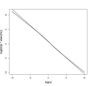
Figure 1: Approximate linear relationship of the logit acceptance rate and the log of the step size.

Plotting the logit of $\frac{2}{\pi}\arctan(\frac{2}{s})$ against $\log(s)$ demonstrates the very close approximate linearity; see Figure 1. Denote this function by $p_{1}(s)$; the subscript $1$ refers to the standard deviation of the posterior distribution. We have

$$\mbox{logit}\ p_{1}(s)\simeq 0.76-1.12\log(s)$$

using a least squares fit of the numerically integrated function. Observe further that, since clearly $p_{\sigma}(s)=p_{1}(s/\sigma)$, we have

$$\mbox{logit}\ p_{\sigma}(s)\simeq 0.76-1.12\log(s/\sigma)=(0.76+1.12\log\sigma)-1.12\log s,$$

so that the slope of the relationship is nearly equal to the constant $-1.12$, independently of $\sigma$. Clearly, this result holds for other means for $x$, and one expects the same result to hold where $x$ is a single component of a parameter with a(n approximately) multivariate normal posterior. Therefore, to find an appropriate step size for an approximately normal marginal distribution, one can consider collecting acceptance rate data for various step sizes and fitting a logistic regression with known slope. The marginal distribution does not need to be very close to normal, either: for example, simulations indicate that the slope for an exponential posterior distribution is about $-1.08$, and so is the slope for a $t$ distribution with $2$ degrees of freedom. These slopes are close enough to $-1.12$ that it is better to use the fixed slope than to try to estimate a slightly different one using data.

Certainly, one could use the actual arctangent relationship to try to choose a good $s$: in the univariate example, if $p$ is the desired acceptance rate, then we obtain $s=2\sigma/\tan(\frac{\pi}{2}p)$, where $\sigma$ is the posterior standard deviation, so we only need to estimate $\sigma$. (Examples of results include $s=2.4\sigma$ for $p=0.44$, $s=3.1\sigma$ for $p=1/e$, and $s=5.3\sigma$ for $p=0.23$.) However, in variable-at-a-time random walk Metropolis updates, one expects that the proper interpretation of $\sigma$ is not the posterior standard deviation but the average conditional standard deviation, which is presumably more difficult to estimate from a Metropolis algorithm.

In our experience, this approach works equally well for positive parameters updated on the log scale with

$$T(x,y)=(2\pi s)^{-1/2}y^{-1}\exp\{-(\log y-\log x)^{2}/2s^{2}\}$$

and with parameters in $(0,1)$ updated on the logit scale with

$$T(x,y)=(2\pi s)^{-1/2}[y(1-y)]^{-1}\exp\{-(\mbox{logit }y-\mbox{logit }x)^{2}/2s^{2}\}.$$

We essentially always update standard deviation parameters, and, respectively, probability parameters in these ways. Our approach also works well if the parameter $x$ is a vector of probabilities that sum to one, and if we propose a new value by adding a Gaussian perturbation to $\mbox{logit }x_{i}$ and rescaling the other $x_{j}$’s so that they still sum to one (and we have a step like this for each $i$).

2.1 Trial stage and logistic regression

To take advantage of this relationship, we begin our MCMC algorithm with a trial stage: the user specifies an initial guess for each proposal standard deviation. The trial stage loops through thirteen (for example) logarithmically spaced step sizes fifty times for each, and monitors the number of accepted moves for each step size. If one then overlooks the fact that the slope in this regression can be taken to be known, one can then fit a logistic regression:

$$\mbox{logit}(\mbox{acceptance probability with step size }s)=a+b\log(s)$$

using Newton-Raphson, and use the estimated parameters to try to hit a target acceptance rate $\hat{s}=\hat{b}^{-1}(\mbox{logit}(p_{target})-\hat{a})$. The Newton-Raphson algorithm works as follows. Let $\hat{a}^{(k)}$ and $\hat{b}^{(k)}$ be the estimates of $a$ and $b$ after $k$ iterations. Let $n_{i}$ be the number of trials for the $i$th step size, $x_{i}$ be the number of accepted moves, and $s_{i}$ be the $i$th step size. Let $\hat{p}_{i}^{(k)}=\mbox{logit}^{-1}(\hat{a}^{(k)}+\hat{b}^{(k)}\log s_{i})$ be the estimated acceptance probabilities for step size $i$ after $k$ iterations. Further let $A^{(k)}=\sum_{i}n_{i}\hat{p}_{i}^{(k)}(1-\hat{p}_{i}^{(k)})$, $B^{(k)}=\sum_{i}n_{i}(\log s_{i})\hat{p}_{i}^{(k)}(1-\hat{p}_{i}^{(k)})$, and $C^{(k)}=\sum_{i}n_{i}(\log s_{i})^{2}\hat{p}_{i}^{(k)}(1-\hat{p}_{i}^{(k)})$. The Newton–Raphson equations are

$$\hat{a}^{(k+1)} = a^{(k)}+\{A^{(k)}\sum_{i}(x_{i}-n_{i}\hat{p}_{i}^{(k)})-B^{(k)}\sum_{i}(\log s_{i})(x_{i}-n_{i}\hat{p}_{i}^{(k)})\}/(A^{(k)}C^{(k)}-B^{(k)2})$$

$$\hat{b}^{(k+1)} = b^{(k)}-\{B^{(k)}\sum_{i}(x_{i}-n_{i}\hat{p}_{i}^{(k)})+C^{(k)}\sum_{i}(\log s_{i})(x_{i}-n_{i}\hat{p}_{i}^{(k)})\}/(A^{(k)}C^{(k)}-B^{(k)2}).$$

In practice, this algorithm converges quickly (in less than twenty iterations) with starting values $a^{(0)}+b^{(0)}=0$, for essentially all the data we have tried.

This algorithm has been implemented in YADAS in case we find an application where the logistic slope differs substantially from -1.12. Most often, though, one should fix the slope and estimate the intercept alone. Using the notation above, the algorithm then updates the intercept $a$ as follows:

$$a^{(k+1)}=a^{(k)}+\frac{\sum_{i}n_{i}(\frac{x_{i}}{n_{i}}-\hat{p}_{i}^{(k)})}{\sum_{i}n_{i}\hat{p}_{i}^{(k)}(1-\hat{p}_{i}^{(k)})}.$$

This algorithm is less numerically stable. It can diverge readily, even when the algorithm is augmented by step halving when the change to $a$ shrinks the likelihood. For this and other reasons, we actually perform the estimate with a “prior” for $a$ included for regularization purposes. A normal prior with mean $\mu_{a}=-3$ and standard deviation $\sigma_{a}=5$ implies that the optimal step size will normally be between $10^{-5}$ and $10^{3}$, and modifies the updating algorithm for $a$ to

$$a^{(k+1)}=a^{(k)}+\frac{\sum_{i}n_{i}(\frac{x_{i}}{n_{i}}-\hat{p}_{i}^{(k)})-\frac{a^{(k)}-\mu_{a}}{\sigma_{a}^{2}}}{\sum_{i}\hat{n}_{i}\hat{p}_{i}^{(k)}(1-\hat{p}_{i}^{(k)})+\frac{1}{\sigma_{a}^{2}}}.$$

One may note that an experiment with thirteen different step sizes may be very conservative compared to what is actually required. In principle, since the slope is known, if one knows the acceptance rate accurately for one step size, one can use that information alone to tune it to a different acceptance rate. However, spending a few hundred iterations in this manner has not seemed overly expensive to us, since we normally run the algorithm for many more iterations after tuning.

2.2 Simulation experiment

Here we discuss a simulation experiment that explores how accurate the initial guesses for step sizes need to be, and how many logarithmically spaced step sizes and how many attempted steps at each step size are needed. Our experiment assumed that the logistic regression model was correct, and that the acceptance rate for step size $s$ is $\mbox{logit}^{-1}\{-5.7-1.12\log(s)\}$; the constants were chosen so that the “optimal” step size is 0.01. The full factorial simulation experiment tried initial guesses of $0.01\times 2^{k}$ for $k=\{-7,-6,\ldots,0,\ldots,6,7\}$, $3,5,7,9,11,13,$ and $15$ different step sizes per run, and 10,20,30,40, and 50 attempted steps per step size. (For example, suppose that the initial guess was 0.16 and the number of step sizes was 9. The step sizes considered would be $0.01,0.02,0.04,0.08,0.16,0.32,0.64,1.28,$ and $2.56$. These step sizes yield acceptance rates of $0.368,0.700,0.903,0.974,0.993,0.998,1.000,1.000,$ and $1.000$.) For each combination of these variables, we constructed 100 simulated data sets using the logistic regression model, estimated $a$ with fixed $b=-1.12145$ using the Newton–Raphson algorithm, recommended a step size based on the estimated $a$ and $b$, and counted how many times out of 100 the recommended step size would generate an acceptance rate between $0.25$ and $0.45$. (For the example with initial guess 0.16 and nine step sizes, the number of “successes” with 10, 20, 30, 40, and 50 attempts per step size were 73, 88, 84, 92, and 91 respectively.) The simulation results are a little erratic to report: the discreteness of the possibilities means that by chance a good step size can be chosen although the data are inadequate. For example, if the initial guess is $0.01\times 2^{7}$, we only attempt three step sizes ten times each, and we get zero acceptances at each step size (which happens about $92\%$ of the time), the algorithm will choose a step size of 0.011, for an acceptance rate of $34\%$. The designs adjacent to this case all have essentially zero probability of getting an acceptable step size. Less severe nonmonotonicities exist as well.

We assume that the initial guess at the step size is off by a given power of two, and report the total trial sample size that yields a success rate (acceptance rate between 25 and $45\%$) of at least $95\%$. If one’s initial guess is exactly right, a total sample size of 120-180 is adequate, and most efficient is 40 trials at each of three step sizes. Not surprisingly, this minimal number of step sizes ceases to be efficient quickly when one’s initial guess is off. When the initial guess is too large by a factor of two, roughly 200 total trials are needed, and there are several equally efficient ways of getting there: 20 each at 9 or 11 levels, 30 each at 7 levels, or 40 at 5 levels. When the initial guess is too high by a factor of 4, 8, 16, or 32, 20 trials at each level are appropriate, and the number of levels should be 11, 11, 13, and 15 respectively: the number of levels needs to be large enough so that at least two step sizes smaller than the optimal are attempted. Overestimating the step size by a factor of 64 can be overcome with 30 trials at each of 15 levels, and an overestimate by a factor of 128 should be avoided.

The situation is not symmetric when one underestimates the optimal step size: in fact, it is better to underestimate it a bit, which is unsurprising since lower step sizes imply acceptance rates of closer to $0.5$, making each trial more informative. Forty trials at each of three levels continues to work well if the initial guess is too low by a factor of two or four. Underestimates of factors of 8, 16, and 32 require total sample sizes of about 180, 220, and 280 respectively, and any choice 20, 30, or 40 per step size is about equally effective.

Of course, one may desire a lower or higher than $95\%$ probability of getting an acceptance rate between $25\%$ and $45\%$. YADAS uses thirteen levels and sample sizes of 50 at each level, and this leads to zero failures in practice even when there are hundreds of parameters. YADAS also sends the chosen step sizes to output files.

3 Implementation

In this section we discuss the YADAS classes that can be used to tune step sizes. For an introduction to YADAS’s software design, please see Graves (2001, 2003, 2007).

In YADAS, the definition of an algorithm is a collection of objects implementing the MCMCUpdate interface. YADAS loops through this collection of updates, calls the update() method of each, and each of these attempts to change the values of one or more unknown parameters. One complete cycle through the collection of updates is one iteration in the MCMC algorithm, and the current values of the parameters are then sent to output files. The simplest example of a object implementing the MCMCUpdate interface is a parameter. A parameter’s update() method loops through the components in the parameter, attempting a Gaussian random walk Metropolis move to each. Another type of update is the MultipleParameterUpdate, which has the capability of proposing a Metropolis or Metropolis–Hastings move that affects multiple parameters simultaneously: the proposed move is defined using a Perturber.

3.1 UpdateTuner

To introduce step size tuning to YADAS, we built a class called UpdateTuner that itself implements MCMCUpdate and can be inserted into the collection of updates in a YADAS algorithm. The UpdateTuner supervises another update, altering its step sizes and monitoring its acceptance rates during a trial phase, analyzing the results of the trial experiment, and then selecting step sizes for the final phase of the MCMC algorithm. To define an UpdateTuner, one specifies:

• An object implementing the TunableMCMCUpdate interface, which will be described below: this is the update step whose step size we are trying to tune. A TunableMCMCParameter is an example of such an object;

• an array of initial guesses for step sizes, one for each step in the update;

• an integer defining the number of trial step sizes to use in the experiment;

• an integer defining the number of attempts per trial step size; and

• a target acceptance rate (we typically use $1/e$).

The last five of these arguments can be omitted; they have default values of: the step sizes assigned to the update, 13, 50, 1, and $1/e$.

3.2 TunableMCMCUpdate

The TunableMCMCUpdate interface extends the MCMCUpdate interface in the following way. It introduces several new methods:

• getStepSizes() returns a vector of doubles, the values of the step sizes currently used by the update. This is actually not used by the UpdateTuner class so may disappear.

• setStepSize has two signatures; one changes a single step size, the other the entire vector.

• acceptances() returns a vector of numbers of acceptances, one for each step size.

• tuneoutput() writes the ultimately selected step sizes to a file with extension .tun.

If a user wants to write a new type of update and wants it to be tunable, the user must ensure that the new update includes appropriate definitions for all these methods. Important update classes that are tunable are MCMCParameter and, unsurprisingly, TunableMultipleParameterUpdate.

3.2.1 Additions to MCMCParameter

We included all the tuning code in the MCMCParameter class itself rather our first intention, which was to have a TunableMCMCParameter subclass. The TunableMCMCUpdate methods do reasonable things. An MCMCParameter includes a vector of unknown scalar parameters, each of which has a step size, and these are the step sizes that are accessed.

Defining parameters in a YADAS application with tuning is identical to applications without, the only exception being that the step sizes included in the definition of a parameter are initial guesses only.

3.2.2 TunableMultipleParameterUpdate

In YADAS, one may add steps to an MCMC algorithm that (attempt to) improve mixing by moving multiple parameters together. This functionality is centered in the MultipleParameterUpdate class, and especially the Perturber interface. A MultipleParameterUpdate consists only of an array of parameters and a Perturber. The Perturber includes all the specialization, such as the method perturb(), which produces proposed new values of the parameters, given their old values, and also calculates the ratio of proposal probabilities that appears in the acceptance rate for Metropolis–Hastings moves. The perturb() method frequently depends on one or more tunable step sizes. A canonical example is the NewAddCommonPerturber. It is quite common that a posterior distribution is approximately a function of differences of some parameters, so that the posterior is relatively insensitive to transformations that add a common constant to all those parameters. This is what NewAddCommonPerturber does: it samples a random Gaussian $Z$ with some standard deviation $s$, and proposes a Metropolis move in which several parameters are incremented by $Z$. More generally, the parameters can be divided into groups, each of which gets its own random $Z_{j}$ and each of which has its own standard deviation $s_{j}$. In this case we want to tune the $s_{j}$’s.

All the Perturbers included in the YADAS package are tunable. We did not include the tuning capability in the Perturber interface itself (rather it is in the TunablePerturber interface) because we didn’t want to make it more difficult than necessary for users to write new Perturbers, but we will try to ensure that the ones we write are as usable as possible, and that includes making them tunable.

YADAS also includes a class ReversibleJumpUpdate which is not yet tunable; further study is required before it is clear that tuning acceptance rates is appropriate in reversible jump problems.

4 Examples

Finally, in this section, we present some examples of the tuning process in practice. First, we work with a normal example with unknown mean and variance and tune both step sizes. Second, we work with a one-way ANOVA that has been parameterized poorly with resultant poor mixing, fix the mixing with a MultipleParameterUpdate, and tune its step size along with the others in the problem. The source code and data for these examples are available on the YADAS website yadas.lanl.gov; follow the “Download” link and then download the zipped directory of examples.

4.1 Normal example

In this problem, Example 10 on the YADAS web site, we have data $y_{i}\sim N(\mu,\sigma^{2})$ for $i=1,\ldots,N$, with priors $\mu\sim N(a_{\mu},b_{\mu}^{2})$ and $\sigma\sim\Gamma(a_{\sigma},b_{\sigma})$ (according to our parameterization, $\sigma$ has prior mean $a_{\sigma}b_{\sigma}$). Each iteration in the MCMC algorithm has two steps: a Metropolis move in which we propose a Gaussian random walk move to $\mu$ (i.e. $\mu^{\prime}=\mu+s_{1}Z_{1}$, where $Z_{1}\sim N(0,1)$, and a Metropolis–Hastings move in which we propose a lognormal adjustment to $\sigma$ (i.e. $\sigma^{\prime}=\sigma\exp(s_{2}Z_{2})$, where $Z_{2}\sim N(0,1)$. $s_{1}$ and $s_{2}$ must be tuned.

The key piece of code in the tuning application is

MCMCUpdate[] updatearray = new MCMCUpdate[]
{ new UpdateTuner(mu, d0.r("mumss"), 13, 50, 1, Math.exp(-1)),
  new UpdateTuner(sigma, d0.r("sigmamss"), 13, 50, 1, Math.exp(-1)) };

in which we define the algorithm to consist of two update steps as described above, and whose step sizes will be tuned. Beginning with the first UpdateTuner, mu is the definition of the update step (here, a Gaussian random walk update to $\mu$). The expression d0.r(‘‘mumss’’) defines a vector of initial guesses for step sizes (only one here, and this expression gets them from an input file). The 13 refers to the number of different step sizes to experiment with, the experiment will attempt 50 moves for each step size, the 1 means only one cycle of experimentation, and the last argument implies that the step size will be tuned for an acceptance rate of $1/e$. The fact that $\sigma$ will be updated using Gaussian random walk moves on the $\log$ scale has been determined elsewhere (sigma was defined to be a MultiplicativeMCMCParameter instead of just a MCMCParameter).

4.2 Badly parameterized one-way ANOVA example

This example, Example 11 on the YADAS website, shows that the tuning procedure works even in cases where multiple parameters are updated at once. This is a one-way analysis of variance example that is commonly used to illustrate mixing difficulties in MCMC algorithms that can be solved with reparameterization. Data $y_{ij}$ are normal with means $\mu_{i}$ and common standard deviation $\sigma$ for $i=1,2,\ldots,I$ and $j=1,2,\ldots,n_{i}$. Here we have taken the $\mu_{i}$ to have a $N(\theta,\delta^{2})$ prior, $\theta$ has a flat hyperprior, and $\sigma$ and $\delta$ have Gamma priors. This parameterization works fine except when $\delta$ is too small compared to $\sigma$ (the sample sizes also drive what is meant by “too small”). In this case, the $\mu_{i}$ and $\theta$ have high posterior correlation so that it works poorly to update them individually. Many solutions exist including reparameterization or block Gibbs updates, but here we use a MultipleParameterUpdate that augments the standard variable-at-a-time Gaussian random walk Metropolis with an additional step that proposes adding a common random Gaussian perturbation to all the $\mu_{i}$ and $\theta$. The posterior distribution is relatively invariant to moves like this, at least when $\delta$ is small, as it is in the supplied input files. The code to define the update algorithm is as follows:

MCMCUpdate[] updatearray = new MCMCUpdate[] {
    new UpdateTuner (mu), new UpdateTuner (theta),
    new UpdateTuner (sigma), new UpdateTuner (delta),
    new UpdateTuner ( new TunableMultipleParameterUpdate
        ( new MCMCParameter[] {mu, theta},
          new NewAddCommonPerturber ( new int[][] { d2.i(0), d0.i(0) },
                                      d0.r("mtmss") ), direc + "mtu") ) };

Here we have used the default values for the experimental design descriptors (13 different trial step sizes for 50 attempts each, and so on). This example successfully tunes a total of four scalar parameters that are updated on the linear scale, two updated on the log scale, and one multiple parameter update. Trace plots of the MCMC iterations are shown in Figure 2.

Figure 2: Trace plots for $\mu_{1},\theta,\log\sigma,$ and $\log\delta$ in the one–way ANOVA example.

5 Conclusions

There are many other effective ways of tuning step sizes in MCMC algorithms; we do not claim that our method is substantially superior to the alternatives, but it is simple, intuitive, and versatile. We readily admit that many problems (for example, those with posterior distributions with curved contours or multiple separated modes) generally feature MCMC difficulties that cannot be adequately solved by tuning step sizes alone. However, our method works well for even a large number of tuning parameters and in a variety of posterior distributions.

References

Andrieu, C. and Thoms, J. (2008). A tutorial on adaptive MCMC. Statistics and Computing 18: 343-373.

Gelman, A.B., Carlin, J.S., Stern, H.S., and Rubin, D.B. (1995). Bayesian Data Analysis, Chapman and Hall/CRC, Boca Raton.

Gelman, A., Roberts, G.O., and Gilks, W.R. (1995). Efficient Metropolis jumping rules. In Bayesian Statistics 5 (J.M. Bernardo, J. Berger, A.P. Dawid, and A.F.M. Smith, eds.) Oxford: Oxford University Press.

Graves, T.L. (2001) “YADAS: An Object-Oriented Framework for Data Analysis Using Markov Chain Monte Carlo,” Los Alamos National Laboratory Technical Report LA-UR-01-4804.

Graves, T.L. (2003). “An Introduction to YADAS,” yadas.lanl.gov.

Graves, T.L. (2007). Design Ideas for Markov Chain Monte Carlo Software.Journal of Computational and Graphical Statistics 16:24-43.

Graves, T.L., Speckman, P.L., and Sun, D. (2004). “Characterizing and eradicating autocorrelation in MCMC algorithms for linear models,” Los Alamos National Laboratory Technical Report LA-UR-04-0486.

Pasarica, C. and Gelman, A. (2010). Adaptively scaling the Metropolis algorithm using expected squared jumped distance. Statistica Sinica 20, 343-364.

Roberts, G.O. and Rosenthal, J.S. (2001). Optimal scaling for various Metropolis–Hastings algorithms, Statistical Science 16, 351–367.

Sherlock, C., Fearnhead, P., and Roberts, G.O. (2010). The random walk Metropolis: linking theory and practice through a case study. Statistical Science 25: 172-190.

Yeung, S.K.H. and Wilkinson, D.J. (2002). Adaptive Metropolis-Hastings samplers for the Bayesian analysis of large linear Gaussian systems. Computing Science and Statistics 33: 128-138.