Switching dynamics in cholesteric blue phases

A. Tiribocchi^∗a, G. Gonnella^a, D. Marenduzzo^b, and E. Orlandini^c

Received Xth XXXXXXXXXX 20XX, Accepted Xth XXXXXXXXX 20XX
First published on the web Xth XXXXXXXXXX 200X

DOI: 10.1039/b000000x

Blue phases are networks of disclination lines, which occur in cholesteric liquid crystals near the transition to the isotropic phase. They have recently been used for the new generation of fast switching liquid crystal displays. Here we study numerically the steady states and switching hydrodynamics of blue phase I (BPI) and blue phase II (BPII) cells subjected to an electric field. When the field is on, there are three regimes: for very weak fields (and strong anchoring at the boundaries) the blue phases are almost unaffected, for intermediate fields the disclinations twist (for BPI) and unzip (for BPII), whereas for very large voltages the network dissolves in the bulk of the cell. Interestingly, we find that a BPII cell can recover its original structure when the field is switched off, whereas a BPI cell is found to be trapped more easily into metastable configurations. The kinetic pathways followed during switching on and off entails dramatic reorganisation of the discli nation networks. We also discuss the effect of changing the director field anchoring at the boundary planes and of varying the direction of the applied field.

1 Introduction

In many cholesteric liquid crystals (CLC) the transition between the regular cholesteric phase and the isotropic phase occurs through a cascade of intermediate phases known as “blue phases” (BP) ¹. Blue phases occur because the locally energetically favoured double twisting (i.e. local twisting in two directions, as opposed to the single twist of the cholesteric) is incompatible with the requirement of continuity ¹. This results in the formation of networks of defects that separate isolated stable regions. The network can lead to quite intricate structures that are periodic at length scales comparable to the wavelength of light – this fact is at the origin of their name (indeed blue phases can be of many different colours).

For example the BPI and BPII phases have a 3D cubic orientational order with lattice periods of several hundred nanometres, and they exhibit selective Bragg reflections in the range of visible light. For this reason they have interesting applications in fast light modulators ^{2, 3} or tunable photonic crystals ⁴. Blue phases are in general thermodynamically stable over a narrow temperature range but recently their stabilization over a range of more than 60 K, including room temperature, have been shown ^{5, 6, 7, 8}. This has opened up new avenues in liquid crystal technologies culminating in the recent fabrication of a blue-phase display device with very fast switching and response times ⁹.

Blue phases are fully 3D structures and the understanding of even their statics is quite a difficult task to achieve that requires very refined techniques and important computational efforts. For these reasons theoretical investigations of blue phases in presence of an electric field have been essentially restricted to the case of infinite samples. Furthermore, typically analytical and semi-analytical theories have focused on the case in which the electric field is infinitesimally small ^{10, 11}. This is in contrast with the experimental characterization of the known blue phases in electric and magnetic fields ^{12, 13, 14, 15}.

Therefore here we aim to investigate the switching dynamics of cholesteric blue phases in an electric field, by numerically solving the hydrodynamic equations of motion for BPI and BPII. The choice of a realistic boundary condition is far from trivial in our system, and in this work we will compare and discuss different possibilities. We first focus on the cases in which the director field is fixed at the top and bottom boundaries ($z=0$ and $z=L$ respectively, where $L$ is the sample size), to its stable structure in the absence of a field – this may in practice be achieved by pinning due to impurities or via surface “memory” effects . We consider the switching dynamics both with an electric (or magnetic) field can be switched on either along the $[0,0,1]$ $z$ direction or along the $[1,1,1]$ diagonal of the unit cell (Section IIIB). Since in practice the orientation of the director field at the boundaries can be controlled and varied (for example by rubbing the plates or treating them chemically), we then investigate the effect that different alignments conditions at the boundaries may have on the structure in the absence and presence of a field (Section IIIC). With respect to previous work on blue phases in electric fields ^{20, 21, 22, 23, 24, 25, 26}, our work considers hydrodynamic interactions, and focuses on switching on and off dynamics in a confined as opposed to a bulk system. This case should be relevant to devices which are typically in the $\mu$m range.

A general picture that emerges out of this study is that the switching is intimately interconnected with the dynamics of the disclination network constituting these phases. For example we show that, under a small field, the disclination network of BPI twists and that of BPII stretches and unzips at the center. Above a given threshold of the voltage, in both cases the network breaks down. The disclinations then pin to the boundaries (we restrict ourselves to the case in which the BP texture is anchored at the top and bottom plates). For BPII we observe that the breaking and pinning dynamics involve the creation of a disclination loop in the middle of the sample. This indeed allows the rotation of the disclination pattern at the boundaries preserving its continuity. As the field is switched off, the structure goes back to the original state or to a cholesteric structure according to the steady state attained with the field on. Measurements of the time evolution of the free-energy of the system allow to characterize the intermediate states reached by the system during the switching on and off cycles.

2 Models and methods

Equilibrium properties of blue phases are described by a Landau-de Gennes free energy density written in terms of the tensor order parameter $Q_{\alpha\beta}$ ^{19, 27, 1}. This comprises a bulk term

$$f_{b}=\frac{A_{0}}{2}(1-\frac{\gamma}{3})Q_{\alpha\beta}^{2} - \frac{A_{0}\gamma}{3}Q_{\alpha\beta}Q_{\beta\gamma}Q_{\gamma\alpha}$$

$$+ \frac{A_{0}\gamma}{4}(Q_{\alpha\beta}^{2})^{2},$$

and a distortion term ¹

$$f_{d}=\frac{K}{2}(\partial_{\beta}Q_{\alpha\beta})^{2}+\frac{K}{2}(\epsilon_{\alpha\zeta\delta}\partial_{\zeta}Q_{\delta\beta}+2q_{0}Q_{\alpha\beta})^{2},$$ (2)

where $K$ is the elastic constant and the pitch of the cholesteric liquid crystal is given by $p\equiv 2\pi/q_{0}$. The tensor $\epsilon_{\alpha\zeta\delta}$ is the Levi-Civita antisymmetric third-rank tensor, $A_{0}$ is a constant and $\gamma$ controls the magnitude of order (it plays the role of an effective temperature for thermotropic liquid crystals). Notice that the magnitude of order, $q(\vec{r})$ (which lies between $0$ and $1$), is $3/2$ times the largest eigenvalue of ${\bf Q}$.

The anchoring of the director field on the boundary surfaces to a chosen director $\hat{n}^{0}$ is ensured by adding the surface term

$$f_{s} = \frac{1}{2}W_{0}(Q_{\alpha\beta}-Q_{\alpha\beta}^{0})^{2}$$ (3)

$$Q_{\alpha\beta}^{0} = S_{0}(n_{\alpha}^{0}n_{\beta}^{0}-\delta_{\alpha\beta}/3)$$ (4)

where the parameter $W_{0}$ controls the anchoring strength, while $S_{0}$ determines the degree of the surface order. If the surface order is equal to the bulk order, $S_{0}$ should be taken equal to $\bar{q}=1/2$ (the value of $q(\vec{r})$ in the bulk, away from disclinations). In the case of strong anchoring $W_{0}$ is practically set to infinity, which means that the order parameter ${\bf Q}$ is fixed on the surfaces – this is how we imposed the anchoring in our simulations.

The last contribution to the free-energy is given by $-(\epsilon_{a}/12\pi)E_{\alpha}Q_{\alpha\beta}E_{\beta}$, and describes the interactions with an external electric field $E$, where $\epsilon_{a}>0$ is the dielectric anisotropy of the liquid crystal. The reduced potential is $\Delta V_{z}=E_{z}L_{z}$, where $E_{z}$ is the component of the electric field along the $x$-direction and $L_{z}$ is the size of the cell in the same direction. Similar expressions can be written for the $x$ and the $y$ components. The time evolution of the system is then governed by the equation of motion for the order parameter ^{28, 18},

$$(\partial_{t}+{\vec{u}}\cdot{\bf\nabla}){\bf Q}-{\bf S}({\bf W},{\bf Q})=\Gamma{\bf H}$$ (5)

where $\Gamma$ is a collective rotational diffusion constant. The first term on the left-hand side of Eq. (5) is the material derivative describing the usual time dependence of a quantity advected by a fluid with velocity ${\vec{u}}$. Since for rod-like molecules the order parameter distribution can be both rotated and stretched by flow gradients ²⁸ a second term must be added to the material derivative:

$${\bf S}({\bf W},{\bf Q}) = (\xi{\bf D}+{\bf\omega})({\bf Q}+{\bf I}/3)+({\bf Q}+{\bf I}/3)(\xi{\bf D}-{\bf\omega})$$ (6)

$$- 2\xi({\bf Q}+{\bf I}/3){\mbox{Tr}}({\bf Q}{\bf W})$$

where Tr denotes the tensorial trace, while ${\bf D}=({\bf W}+{\bf W}^{T})/2$ and ${\bf\omega}=({\bf W}-{\bf W}^{T})/2$ are the symmetric and the anti-symmetric part of the velocity gradient tensor $W_{\alpha\beta}=\partial_{\beta}u_{\alpha}$. The constant $\xi$ depends on the aspect ratio of the molecules forming a given liquid crystal. This parameter controls whether the director field is flow aligning in shear flow ($\xi>\frac{3\bar{q}}{2+\bar{q}}$), creating a stable response, as opposed to flow tumbling, which gives an unstable response ($\xi<\frac{3\bar{q}}{2+\bar{q}}$).

The molecular field ${\bf H}$, which provides the driving motion towards the minimum of the free energy, is given by

$${\bf H}=-{\delta{\cal F}\over\delta{\bf Q}}+({\bf I}/3)Tr{\delta{\cal F}\over\delta{\bf Q}}.$$ (7)

The fluid velocity, $\vec{u}$, obeys the continuity equation and the Navier-Stokes equation, which in the incompressibile fluid limit reads

$$\rho(\partial_{t}+u_{\beta}\partial_{\beta})u_{\alpha}=\partial_{\beta}(\Pi_{\alpha\beta})+\eta\partial_{\beta}(\partial_{\alpha}u_{\beta}+\partial_{\beta}u_{\alpha}).$$ (8)

with a stress tensor generalized to describe the flow of cholesteric liquid crystals, and equal to

$$\Pi_{\alpha\beta}= - P_{0}\delta_{\alpha\beta}+2\xi(Q_{\alpha\beta}+{1\over 3}\delta_{\alpha\beta})Q_{\gamma\epsilon}H_{\gamma\epsilon}$$

$$- \xi H_{\alpha\gamma}(Q_{\gamma\beta}+{1\over 3}\delta_{\gamma\beta})-\xi(Q_{\alpha\gamma}+{1\over 3}\delta_{\alpha\gamma})H_{\gamma\beta}$$

$$- \partial_{\alpha}Q_{\gamma\nu}{\delta{\cal F}\over\delta\partial_{\beta}Q_{\gamma\nu}}+Q_{\alpha\gamma}H_{\gamma\beta}-H_{\alpha\gamma}Q_{\gamma\beta}$$

where $\rho$ is the fluid density and $\eta$ an isotropic viscosity. $P_{0}$ is a constant in the simulations reported here.

Notice that, unless the flow field is zero ($\vec{u}=0$), the dynamics of the order parameter are not purely relaxational. Conversely, the order parameter field affects the dynamics of the flow field through the stress tensor, which depends on the molecular field ${\bf H}$ and on ${\bf Q}$. This is the back-flow coupling. In our simulations, the coupling to hydrodynamics via a non-trivial pressure tensor can be switched off, essentially by imposing a constant zero velocity profile. In this way the effects of flow and backflow may be easily tested.

To solve these equations we use a 3D hybrid lattice Boltzmann algorithm that consists in solving Eq. (5) via a finite difference predictor corrector algorithm while the integration of the Navier-Stokes equation (8) is taken care by a standard Lattice Boltzmann (LB) approach. The hybrid method has the advantage that involves consistently smaller memory requirements with respect to the full LB counterpart ^{29, 30} and its efficiency has been indeed already tested for binary fluids ³¹, nematic devices ³² and active nematic liquid crystals ^{33, 34, 35}.

In our simulations we fixed $\Gamma=0.3$, $\xi=0.7$ and $\eta=1.333$ as suggested by previous experience on numerical investigation of blue phases ³⁶. Typical simulations reported here required about 2000 single processor cpu hours. Most of our runs were parallel (MPI architecture) with 8-16 nodes.

To locate the defects in the simulation domain, we look at the local behaviour of the order, $q(\vec{r})$: namely when $q(\vec{r})$ falls below a predetermined threshold, we identifiy that lattice point as belonging to a disclination. This prescription is very easy to implement and allows a determination of the disclinations that turned out to be as accurate as the more complicated procedure based on the degree of biaxiality ³⁷. For our study we have chosen a threshold of $q=0.19$ that corresponds to the $60\%$ of the largest eigenvalue of ${\bf Q}$ at the steady state. Clearly a variation of the threshold value generally leads to a variation in the thickness of the rendering of the disclinations in the figures.

In our calculations the size of a cubic unit cell has been set equal to $32\times 32\times 32$ in simulation units. Note that the size of the unit cell which minimises the free energy is in general different from the cholesteric pitch – typically it is larger, and this size change has been referred to as “redshift” in the literature ^{36, 39, 38}. In our simulations we have kept the redshift constant to the values suggested in Ref. ³⁶, and valid for zero field. We note that in principle the electric field modifies the optimal redshift in equilibrium ²⁵. While this is important to obtain an accurate phase diagram for blue phases in the bulk, it does not qualitatively affect either the switching dynamics or the behaviour of a confined blue phase in an electric field (we have verified this by running our simulations with no redshift, both the succession of phases in Fig. 1 and the switching dynamics are unaffected).

3 Results

3.1 Steady state in an electric field

The equilibrium structures in the absence of an electric field (Fig. 1a and Fig. 1d) were obtained by relaxing the free energy to its minimum value by solving Eq. (5) numerically. Periodic boundary conditions were employed along the $x$ and $y$ axes, whereas on the $z=0$, $z=L$ planes we fixed the director field as in the bulk equilibrated blue phase configuration. Before the network disrupts, also the experiments in Ref. ⁵ suggest that the texture at the boundaries does not modify so that our assumption should be appropriate. In practice, as commonly assumed in the theory of permeation in cholesterics ^{16, 17, 18}, fixed boundary conditions may be due to pinning of disclinations via surface impurities, or by surface “memory” effects (see below for results with different boundaries and a more thorough discussion of their roles).

When we apply an electric field we initially consider a system with width $L$ equal to the periodicity of the BP structures along z. Initial configurations were set according to the approximate solutions in Ref. ¹. Note that the periodicity of the ground state is related to the blue phase pitch via a non-trivial constant (also known as “redshift”) which we have taken to be equal to the one resulting from the semi-analytical minimisation of the free energy presented in Ref. ^{35, 38, 36, 20}. The structure we get then only depends on the liquid crystal chirality $\kappa$, reduced temperature $\tau$ and on ${\cal E}$ which takes into account electric field effects. These are related to our parameters as

$$\kappa = \sqrt{\frac{108Kq_{0}^{2}}{A_{0}\gamma}}$$ (10)

$$\tau = \frac{27(1-\gamma/3)}{\gamma}+\kappa^{2}$$ (11)

$${\cal E}^{2} = (27\varepsilon_{a}E_{\alpha}E_{\alpha})/(32\pi A_{0}\gamma).$$ (12)

The static phase diagram at ${\cal E}=0$ is in a better agreement with experiments with respect to earlier calculations based on semi-analytical approximations and is given in Refs. ^{38, 36}, where it is shown that BPI and BPII appear in order of increasing values of $\kappa$ as found experimentally.

We have chosen $A_{0}$, $K$ and $\gamma$ in order to be in the appropriate region of the phase diagram. We have set $A_{0}=0.0034$, $K=0.005$, $\gamma=3.775$ for BPI, and $A_{0}=0.00212$, $K=0.005$, $\gamma=2.9$ for BPII. These may correspond, for instance, to a blue phase with lattice constant equal to 400 nm, with a rotational viscosity equal to 1 Poise and (Frank) elastic constants equal to $\sim 10$ pN and $\sim 16$ pN for BPI and BPII respectively, which are in the range of typical liquid crystalline materials. Accordingly, one may calculate that one space and time LB unit correspond to 0.0125 $\mu$m and 0.0013 $\mu$s for BPI, and to 0.0125 $\mu$m and 0.0017$\mu$s for BPII. Furthermore, in order to map electric field related quantities to real units, the best avenue is to use the previously defined dimensionless number ${\cal E}$ and compare simulation and experimental values. An electric field of 1 V/$\mu$m, with a dielectric anisotropy $\sim$ 10, by assuming $\frac{27}{2A_{0}\gamma}\sim 2-5\times 10^{-6}{\rm J}^{-1}\,{\rm m}^{3}$ ¹, would lead, for instance, to ${\cal E}\sim$0.01 whereas a voltage of 0.1 in Fig. 1 corresponds in our simulations to ${\cal E}\sim$0.1 ($\sim$0.09 for BPI and $\sim$0.13 for BPII).

In Fig. 1 we show how the steady state, after the field is switched on, changes as a function of the voltage applied along the $z$ direction. In the case of BPII (top row), for small electric field the steady state is indistinguishable from the starting configuration (Fig. 1a), while above a threshold (a voltage $\Delta V\simeq 0.175$ in simulation units with the parameters we chose, see caption to Fig. 1), the network unzips at the centre (Fig. 1b). For a voltage larger than about 0.3, the disclinations reconstruct at the surface to form an array of straight parallel lines (Fig. 1c). In the case of BPI (bottom row), the zero-field structure (Fig. 1d), is unstable after a first threshold (0.275) and becomes twisted in steady state with a voltage on (Fig. 1e). If the field exceeds a second threshold (about 0.425 in the case of Fig. 1), the network again breaks and the disclinations pin to the boundaries (Fig. 1f).

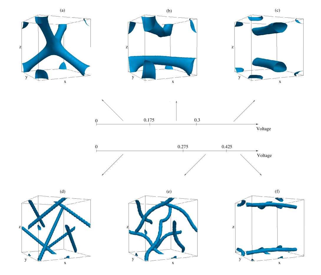
Fig.  1: Steady state disclination networks for BPI and BPII under a varying field, and strong anchoring of the zero-field structure on the surface. BPII structures are shown in the first row, BPI are in the bottom row. The simulation domain has size $32\times 32\times 32$. The range of stability in voltage (simulation units) of each of the networks shown in the snapshots is also indicated. Snapshots correspond to steady states with $\Delta V$ equal to 0 (a,d), 0.3 (b), 0.4 (c); 0.375 (e), 0.5 (f).

The difference in the optical signal transmitted by a liquid crystalline sample between cross polarizers with and without an applied field depends on the difference in the director field profile. Fig. 2 shows the director field on a cut of the sample parallel to the $xy$ plane at $z=L/2$, with different applied voltages. The double twist regions separating the disclination lines - typical of blue phases in equilibrium - are evident from the figure.

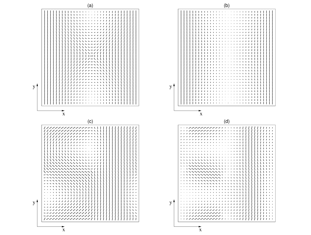
Fig.  2: Director field profiles on the $xy$ plane taken at $z=L/2$. Panels (a) and (b) correspond to the steady state disclination networks of Fig 1a and 1b (BPII). Panels (c) and (d) correspond to Fig. 1d and Fig. 1e (BPI).

3.2 Switching dynamics of blue phase devices

We now discuss the switching on and off dynamics of a blue phase device – focussing on the case of strong anchoring (i.e. $W_{0}>>1$). Fig. 3 (snapshots $t_{0}-t_{5}$) shows the response of a BPII cell to an electric field along the $\hat{z}$ direction. The field is strong enough to pin the disclinations to the surface (see the preceding Section and the discussion of Fig. 1). The disclinations unbind at the centre of the cell soon after the application of the electric field. These then join to the defect at the boundaries, to reconstruct later on via the formation of a loop in the bulk of the sample. Such a remodelling of the defect networks leads to a rotation of the surface disclinations, which end up straight and parallel to each other.

It is interesting to ask what happens to this highly distorted BP cell once the electric field is removed, especially in the high field regime on which we focus later on. Do we get back to the initial BPII configuration, or does the device get stuck into a different metastable configuration? To address these questions, we have simulated the switching off dynamics starting from the configuration shown in Fig. 3, snapshot $t_{5}$. When the electric field is switched off to zero, the defects depin and meet in the bulk (snapshots $t_{6}-t_{7}$). There, they join with the surface defects due to the anchoring to form a fully connected structure with the disclinations closeby in the center of the cell (snapshot $t_{8}$). These then tilt and twist (snapshots $t_{9}-t_{10}$), to finally reform the original structure (snapshot $t_{11}$). Therefore the BPII cell has the potential to be used as an electrically switchable device, provided at least that the original network of defects is pinned to the surface.

Fig. 4 shows the results of an analogous electric field cycle for a BPI cell – note that this is the BP used in the experimentally constructed device in Ref. ⁷. Our results suggest that switching in this disclination network both entails a qualitatively different pathway and leads to a distinct steady state. During switching on ($t_{0}-t_{5}$), the BPI disclinations transiently twist up, as in the steady states shown in Fig. 1. When the twisted defects get close enough, they recombine and once again pin to the boundaries. After the field is switched off ($t_{6}-t_{11}$), different disclinations depin and follow different dynamics: some migrate back to the centre, while others rejoin to neighbouring ones to form either arcs connected to the same surface, or lines spanning the whole device. In this case, then, the network gets stuck “en route” into a metastable state, which is distinct from both the zero and the high field BPI configurations. Despite this, it is still possible to use this BPI cell as a device, which switches between the configurations in $t_{5}$ and $t_{11}$ under the action of an applied field. We have done systematic simulations of several cycles and we have observed that there is a reversible cycle between the field induced state $t_{5}$ and the metastable state $t_{11}$, but the system can not get back to the original BPI defect structure as at $t_{0}$. Therefore the structure is permanently deformed. It may be interesting to systematically scan the chirality–temperature phase space to investigate whether our finding that BPI devices do not switch back to their original, zero field, stable state is robust and generic, or depends on the exact position of the starting state in the phase diagram. To answer this question, we have performed a simulation similar to the one described in Fig. 4 (i.e. field cycle for a BPI phase) but starting from a different point of the phase diagram.

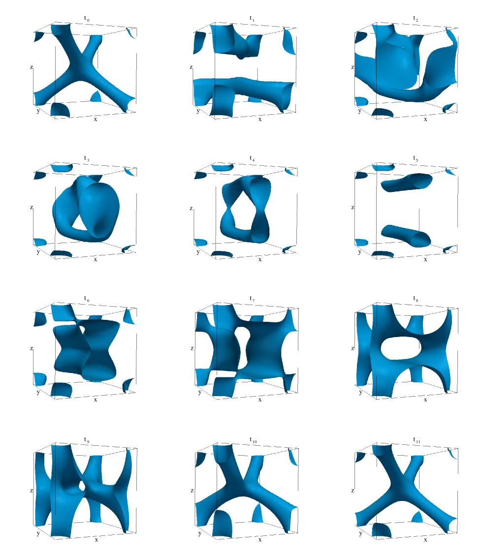
Fig.  3: Evolution of the disclination network of the BPII phase during the switching on ($t_{0}-t_{5}$) -off ($t_{6}-t_{11}$) dynamics in a cell of size $32\times 32\times 32$. Strong anchoring at the $z=0$ and $z=L$ planes are considered. The electric field, applied along the $z$-direction ($[0,0,1]$), is switched on ($\Delta V=0.4$) at $t_{0}=35000$ and switched off at $t_{5}=150000$. After a cycle, the system reforms the original defect structure, as can be seen at time $t_{11}$. For this reason the BPII cell can be used as a switchable device. All the values reported are in simulation units.

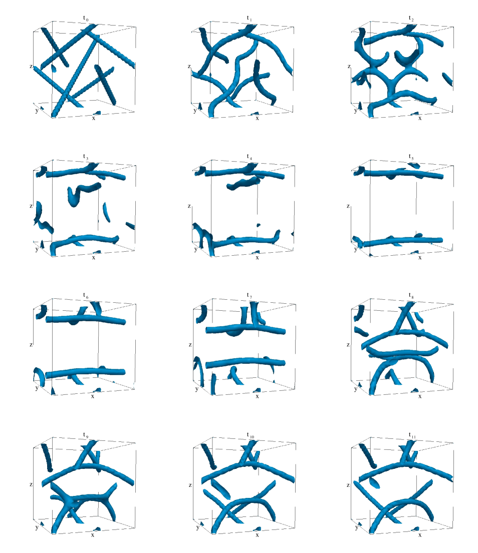
Fig.  4: Evolution of the disclination network of the BPI phase during the switching on ($t_{0}-t_{5}$) -off ($t_{6}-t_{11}$) dynamics in a cell of size $32\times 32\times 32$. Strong anchoring at the $z=0$ and $z=L$ planes are considered. The electric field, applied along the $z$-direction ($[0,0,1]$), is switched on ($\Delta V=0.5$) at $t_{0}=35000$ and switched off at $t_{5}=250000$. The final state at time $t_{11}$ has a different defect structure respect to the typical network of the BPI ($t_{0}$). The free-energies of these two states are different (see Fig. 5) but, after several cycles, the switching is reversible between the states $t_{5}$ and $t_{11}$. All the values reported are in simulation units.

Fig. 5 shows the time behaviour of the free energy for the BPII (left) and the BPI (right) devices corresponding to the switching on-off dynamics of Fig. 3 and 4. In both cases the electric field was applied after $t_{0}=35000$ iterations, and correspondingly the free energy abruptly drops. When the electric field is switched off ($t_{5}=150000$ (left) and $t_{5}=250000$ (right)), the free energy increases abrubtly and then relax down to a new (zero field) steady state. From the inset it is shown that whereas the BPII device is able to get back to the zero field state after removal of the field, the BPI cell gets trapped in a metastable configuration, with free energy slightly larger than that of the stable BPI phase. The failure of the BPI device to come back to its original equilibrium state seems to be quite generic since we observe the same phenomena for a starting state that belongs to a different region of the phase diagram (see squares in Fig. 5 right panel).

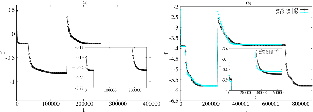
Fig.  5: Time evolution of the free energy of the BPII (left) and BPI (right) phases during the switching on-off dynamics of Fig. 3 and 4. The two insets are zooms of the main figures and show the values of the free energies at the beginning and at the end of the switching on-off cycle. One can notice that, while for BPII the two values are essentially the same, for the BPI phase the final state has a higher values of the free energy (metastable state). This turns out to be true even if we start from initial states belonging to different regions of the phase diagram (open circles and filled squares, see legend for values of $\kappa$ and $\tau$). Open circles correspond to the parameters in Fig. 4; filled squares to $A_{0}=0.0012$, $K=0.005$, $\gamma=5.085$, and other parameters as above.

As the blue phases are anisotropic phases, the orientation of the electric field matters, and we have compared the case presented above in which the field was along the $\hat{z}$ axes to the one in which it is applied along the [111] diagonal of the unit cell. The results are shown in Figs. 6 and 7, for BPII and BPI respectively. Note that here we consider the dynamics for values of the field which are sufficient to break the initial networks, so that these can be compared with the switching dynamics with the field in the [001] direction. The case of a diagonal electric field was previously considered in Ref. ²³, although in that work backflow effects were not implemented and periodic boundary conditions were considered in all directions.

In the case of BPII (Fig. 6), the switching on dynamics is now different. In particular, the network now does not unbind, and the central defect which joins up four disclinations is now stable: it moves along the direction of the field until it touches the surface to recombine into a pair of arcs ($t_{0}-t_{5}$). Once more, when the field is removed the network grows from the surface into the bulk and reconstructs the initial configuration ($t_{6}-t_{11}$).

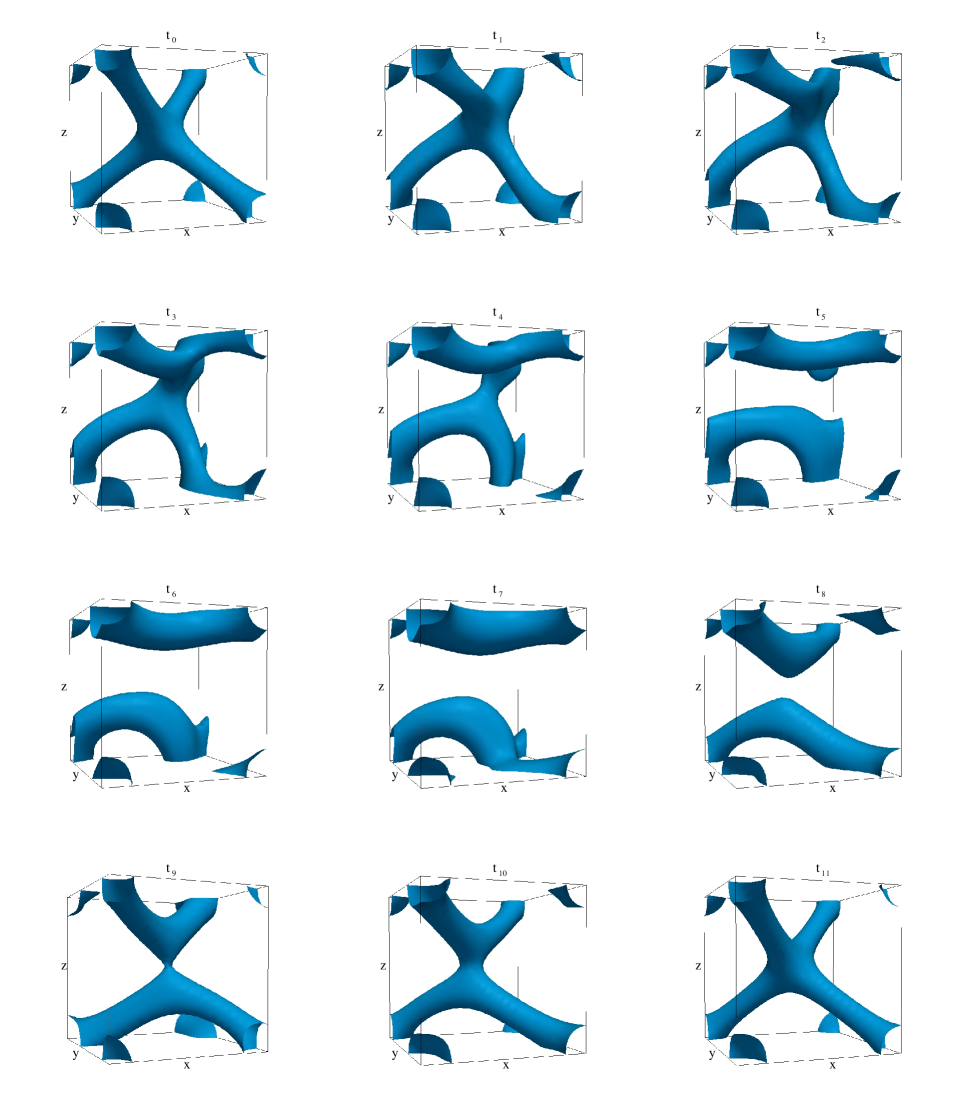
Fig.  6: Evolution of the disclination network of the BPII phase during the switching on ($t_{0}-t_{5}$) -off ($t_{6}-t_{11}$) dynamics in a cell of size $32\times 32\times 32$. Strong anchoring at the $z=0$ and $z=L$ planes are considered. Unlike the case shown in Fig. 3 the electric field is switched on (at $t_{0}=35000$) along the diagonal ([111], pointing vertically and to the right in the picture) of the unit cell ($\Delta V/L_{x}=\Delta V/L_{y}=\Delta V/L_{z}=0.2$). The switching off occurs at $t_{6}=305000$. As in the case in which the electric field is applied along the $z$-direction, here, after a cycle, the network disclination ($t_{11}$) is identical to zero-field configuration observed at time $t_{0}$. All the values reported are in simulation units.

Fig. 7 shows the switching of a BPI cell with a field along the [111] directions. As for the case of the field along [001], the disclination twists in an applied field – remarkably, the one along the field direction however does not ($t_{1}$). When the deformation becomes large enough, the network forms branching points, which are unstable and annihilate in the bulk leaving once more a state with arcs of defects close to the boundaries ($t_{2}-t_{5}$) – this time the state is not symmetric, unlike the analogous case with the field along [001]. The switching off proceeds along a similar pathway as the one shown in Fig. 4, even though the final state is yet different ($t_{6}-t_{11}$).

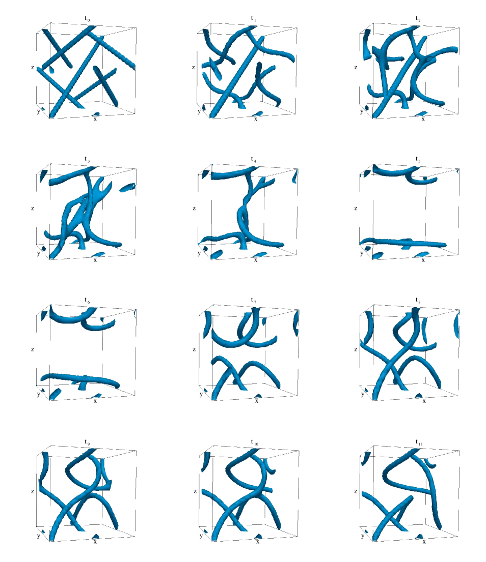
Fig.  7: Evolution of the disclination network of the BPI phase during the switching on ($t_{0}-t_{5}$) -off ($t_{6}-t_{11}$) dynamics in a cell of size $32\times 32\times 32$. Strong anchoring at the $z=0$ and $z=L$ planes are considered. Unlike the case shown in Fig. 4 the electric field is switched on (at $t_{0}=35000$) along the diagonal ([111]) of the unit cell ($\Delta V/L_{x}=\Delta V/L_{y}=\Delta V/L_{z}=0.275$). The switching off occurs at $t_{5}=250000$. Similarly to the case observed in Fig. 4, after a cycle, the system can not recover the zero-field stable confioguration of the defects of the BPI. All the values reported are in simulation units.

In our simulations, we can switch off hydrodynamic interactions, which is often referred to as backflow in the field of liquid crystal dynamics, and therefore unambiguously pinpoint the effect of hydrodynamics. Qualitatively, it is sometimes the case that hydrodynamics allows the kinetics of the system to cross free energy barriers which would otherwise trap it into metastable states. Quantitatively, the relaxation times are usually decreased by backflow, which “speeds up” many processes. Fig. 8 shows the comparison between two switching on and off simulations, one with hydrodynamics and the other without – we considered the case of a BPI cell with field along [001]. It can be seen that hydrodynamics slightly accelerates the dynamics. The steady states are not affected for BPII; they are different for BPI, but are metastable in both cases and very close in free energy.

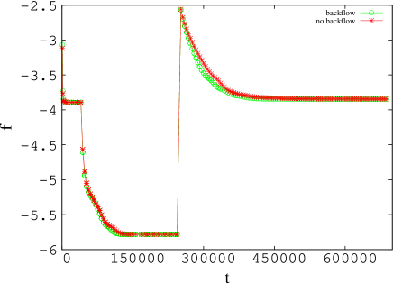
Fig.  8: Time evolution of the free energy of the BPI phase during a switching on-off dynamics. The electric field is taken along the [001] direction. The stars (circles) correspond to the situation withouth (with) hydrodynamics.

3.3 Effect of boundary conditions

We now come back to the important, and non-trivial, issue of the choice of the boundary conditions for our device switching simulations. As mentioned above, fixed boundaries have often been used in the physics of cholesteric liquid crystals and blue phases ^{16, 17, 18, 39}. Indeed, in the case of permeation, fixed boundaries have proved to be closer to rheology experiments than, say, the case in which the director field can rotate freely at the boundary ¹⁸. Still, these boundary conditions are very difficult to exactly enforce in experiments. In practice, as for cholesterics ^{16, 17}, one may envisage that the liquid crystalline texture and disclination pattern may be pinned at least partially by impurities, or it may be kept for some time due to surface “memory” effects which slow down the dynamics close to the boundaries. In the case of our blue phase device, for large electric field the regrowth of a disclination pattern after switching off (BPII or the metastable BPI state in Fig. 4) is likely to be efficient due to the imprinting at the boundaries. To see how realistic this is, one would need experiments like those in Ref. ⁵, but for large electric fields which destroy the initial blue phase at the bulk. For blue phase devices such as those in ⁵ the switching back occurs on the sub-ms scale: if surfaces respond as free boundaries, however, there should be a field above which regrowth is much slower, as it should then occur via nucleation of the stable zero-field blue phase starting from a field-induced metastable state. New experiments would be needed to completely settle this issue.

On the other hand, experimentalists do have at their disposal a range of well developed and established techniques to accurately control the alignment of the director field at the boundaries of a liquid crystalline sample or device. For instance, by rubbing it is possible to obtain a homogeneous anchoring, parallel to the boundary plane, whereas by means of chemical treatment the surface may be made to favour homeotropic, or perpendicular, anchoring. These two anchoring conditions are very much used in practice and, as they are very well controllable, therefore it would be desirable to know what their effect is on the director conformation and switching of blue phase devices. Indeed, some simulations with relatively small sample sizes and no hydrodynamics suggested that at least when the boundaries are close by homeotropic anchoring ²⁴, boundary conditions change the defect structure of a confined BPI phase.

To address the role of homeotropic and homogeneous anchoring on the structure of a BP device at zero applied field, we have numerically simulated the relaxation to equilibrium of three BPI and BPII unit cells, in a $32\times 32\times 96$ simulation domain (the size was increased to minimize the effect of boundary layers). Periodic boundary conditions were applied along the $x$ and $y$ directions, whereas (infinitely) strong homeotropic anchoring was enforced on the $z=0$ and $z=L$ planes. Fig. 9 shows the steady states for BPII (a) and BPI (b) respectively. In both cases, while the bulk of the sample is virtually indistinguishable from an equilibrated BPI/BPII cell, there are strong anchoring driven deformations close to the boundary. In the case of BPII (panel a) these result into the formation of a stack of parallel disclinations confined at the surface and disjointed from the rest of the network. In the BPI cell, on the other hand, the diagonal disclinations approaching the boundaries bend away from these, and again more disclination lines appear at the surfaces, although this time they are not straight, but twisted, and the lines on the two boundaries are perpendicular to each other.

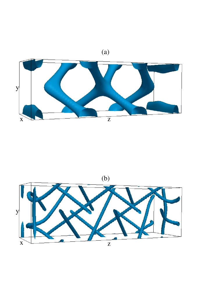
Fig.  9: Steady state disclination networks at zero field for BPI (panel b) and BPII (panel a). The simulation domain has size $32\times 32\times 96$. Periodic boundary conditions are considered along $x$ and $y$ whereas strong homeotrophic anchoring has been enforced on the planes $z=0$ and $z=L$. The effects of boundaries are limited to the size of a single domain. The bulk structure is unaffected while column-like surfaces appear near the boundaries.

Fig. 10 shows the steady state configurations found with homogeneous anchoring, along the $z=0$ and $z=L$ planes. In this case, there are no surface defects disjointed from the bulk of the network, rather the network deforms and reconstructs to join just above the surface and avoids it. As in the homeotropic case, in our 3 cell domain the bulk is basically unaffected by the anchoring, which suggests that surface effects do not appreciably extend over one unit cell.

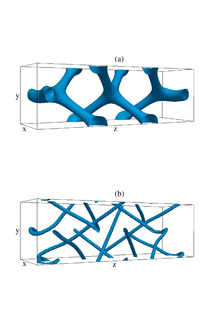
Fig.  10: Steady state disclination networks at zero field for BPI (panel b) and BPII (panel a). The simulation domain has size $32\times 32\times 96$. Periodic boundary conditions are considered along $x$ and $y$, and strong homogeneous anchoring along the $x$ direction has been enforced on the planes $z=0$ and $z=L$.

We have therefore seen that changing anchoring conditions has a strong effect on the zero-field structure of the network close to the surface. What about the behaviour in an electric field? Rather than doing an exhaustive analysis, which is too costly computationally, we have chosen here to focus on one case, that of BPI with homeotropic anchoring. This should be the most interesting case, as hysteresis effects and metastability are more pronounced for BPI. Fig. 11 shows the switching dynamics with $\Delta V=1$. After the field is switched on along the $\hat{z}$ axis, we observe that the bulk disclinations twist, as in the single unit cell simulation (see Fig. 1e), while the twisted defects appearing at the surfaces reorganize as follows: some of them bend and move slightly towards the bulk while the others remain fixed at the boundaries forming column-like structure ($t_{0}-t_{2}$). When the field is switched off ($t_{3}-t_{5}$) the bulk network restructures itself, restoring the usual BPI defect disposition, while at the surfaces only a partial restoration of the defect structure as at $t_{0}$ occurs. Notice that for the voltage chosen here, $\Delta V=1$, in a device with a single unit cell, the disclination network breaks and does not reform (Fig. 1). In the current simulations, however, permanent deformations in the defect structure are observed at the steady state only at the surfaces, while the structure in the bulk is unaffected. We have also performed further simulations with 6 unit cells in the field direction (with a unit cell resolved with 16 instead of 32 lattice points) and homogeneous and homeotropic anchoring. We have studied the case of a very large field which destroys the disclination networks. In this case the network does not reform. This may be seen as a prediction as it is possible to treat boundaries in liquid crystals so as to force such alignments. Our results also suggest that the boundary conditions are not expected to affect the qualitative behaviour of the devices under an electric field, at least up to intermediate values of the electric fields.

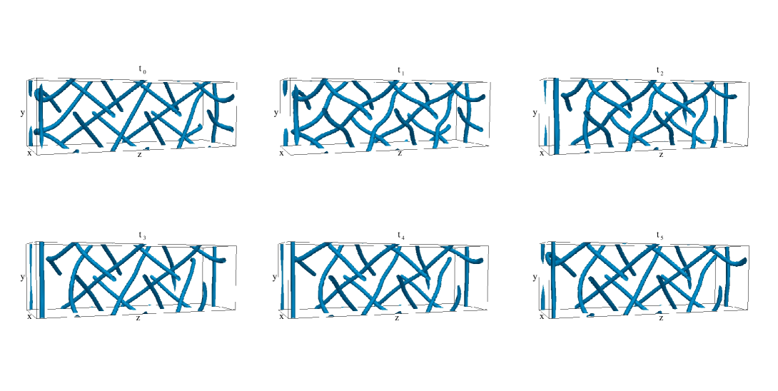
Fig.  11: Evolution of the disclination network of the BPI phase during the switching on ($t_{0}-t_{2}$) -off ($t_{3}-t_{5}$) dynamics. Homeotropic strong anchoring at the $z=0$ and $z=L$ planes are considered. The electric field is switched on ($\Delta V=1.0$) at $t_{0}=120000$ along the [001] (vertical) direction. The field is then switched off at $t_{3}=376000$.

4 Conclusions

In conclusion, we have reported a numerical investigation of electric field induced switching of devices built starting from cholesteric blue phases. At steady state, with a field along the [001] direction (which is normal to the boundary planes), BPII undergoes an “unzipping transition”upon increasing the electric field strength; while BPI twists above a first parameter dependent electric field threshold, then breaks as the field exceeds a second larger critical value. It is likely that the initial deformations of BPII (unzipping) and BPI (twisting) are crossovers or very smooth transitions, whereas the final defect disruption is a sharp transition. The dynamics of the field-induced disruption of the network is very rich.

If the disclinations are fixed at the boundaries by impurities, our simulations predict an intricate pathway which allows the BPII structure to rotate its disclinations once they touch the top and bottom plates via the creation of a disclination loop. Once the field is switched off, we found that, remarkably, the liquid crystal can reform the original blue phase stable at zero field. In the case of BPI, disclinations again twist up and then pin to the boundary. Upon switching off the field, the disclinations unpin and part of the network deforms, although the zero field configuration is not recovered unless the applied field is below a critical threshold. Given the vastly different defect and director configurations, the disclination dynamics predicted numerically should leave observable signatures in experiments.

When the field is along the diagonal of a unit cell, i.e. along [111], the BPII network does not unzip, rather it smoothly deforms until it touches the boundary. The disclinations in BPI, instead, still twist and reconstruct. The different response to the electric fields along [001] and [111] is a result of the anisotropy of blue phases.

In practice, in liquid crystal samples the orientation of the director field at the boundary can be controlled via rubbing or chemical treatment. We have therefore investigated how our results are affected if the director field at the surfaces of the device is anchored and lies either perpendicularly to the surface or along one rubbing axis on the plane. In both cases, there is a boundary layer in which the disclination network reconstructs to either avoid the surface or form pinned disclinations disjoint to the rest of the network. If the device is one unit cell thick only, these deformations lead to new disclination networks, some of which are far from the original BP networks. For thicker devices, on the other hand, the bulk is essentially indistinguistable from the thermodynamically stable phase. In this regime, the switching in an electric field is not very different from the fixed surface boundary conditions. We also find that hydrodynamics, or backflow, has a relativel y minor effects on the switching on and off dynamics.

We hope that our results have shown that it is now possible to qualitatively follow and predict the switching on and off dynamics of BP devices with a variety of boundary conditions. The parameters we have chosen are similar to the typical liquid crystalline ones and the effects observed are expected to be generic and robust for different values of e.g. viscosities and elastic constants. It would also be interesting to study what happens if we relax the one elastic constant approximation alex”. Future experiments would be important to test the current simulation predictions and results, and to suggest further technologically relevant questions.

Acknowledgements

We acknowledge the HPC-Europa2 program for funding a visit of AT to Edinburgh, during which this work was started, and CASPUR in Rome for a grant providing access to their computing facilities. We also warmly thank F. Salvadore, researcher at CASPUR, for help during the first stages of the work.

References

- 1 D. C. Wright, N. D. Mermin, Rev. Mod. Phys. 61, 385 (1989) and references therein.
- 2 V.E. Dmitrenko, Liq. Cryst. 5, 847-851 (1989).
- 3 G. Heppke, B. Jerome, H.-S. Kizerow and P. Pieranski, J. Phys. (Paris) 50, 2991-2998 (1991).
- 4 P. Etchegoin Phys. Rev. E, 62 1435-1437 (2000).
- 5 H. Kikuchi, M. Yokota, Y. Hisakado, H. Yang and T. Kajiyama, Nat. Mater. 1 64 (2002).
- 6 Y. Hisakado, H. Kikuchi, T. Nagamura and T. Kajiyama, Adv. Mat. 17 96 (2004).
- 7 H. J. Coles and M. N. Pivnenko, Nature 436, 997 (2005).
- 8 E. Karatairi, B. Rozic, Z. Kutnjak, V. Tzitzis, G. Nounesis, Phys. Rev. E, 81 041703 (2010).
- 9 www.physorg.com/news129997960.html (2008).
- 10 P. Pieranski, P. E. Cladis, R. Barbet-Massin, J. Phys. (Paris) Lett. 46, L973 (1985).
- 11 P. Pieranski, P. E. Cladis, Phys. Rev. A 35, 355 (1987).
- 12 E.M. Terenthjev Phys. Rev. E, 51 1330-1336 (1995).
- 13 W. Y. Cao, A. Munoz, P. Palffy-Muhoray, B. Taheri B, Nat. Mater. 1, 111-113 (2002).
- 14 H. Stegemeyer, F. Porsch, Phys. Rev. A 30, 3369 (1984).
- 15 N.-R. Chen, J. T. Ho, Phys. Rev. A 35, 4886 (1987).
- 16 W. Helfrich, Phys. Rev. Lett. 23, 372 (1969).
- 17 T. C. Lubenski, Phys. Rev. A 6, 452 (1972).
- 18 D. Marenduzzo, E. Orlandini, J. M. Yeomans, Phys. Rev. Lett 92, 188301 (2004).
- 19 P. G. de Gennes and J. Prost, The Physics of Liquid Crystals, 2nd Ed., Clarendon Press, Oxford (1993).
- 20 D. Lubin, R. M. Hornreich, Phys. Rev. A 36, 849 (1987).
- 21 R. M. Hornreich, M. Kugler, S. Shtrikman, Phys. Rev. Lett. 54, 2099 (1985).
- 22 G. P. Alexander, D. Marenduzzo, EPL 81, 66004 (2008).
- 23 J. Fukuda, M. Yoneya, and H. Yokoyama, Phys. Rev. E 80, 031706 (2009).
- 24 J. Fukuda, S. Zumer, Phys. Rev. Lett. 104, 017801 (2010).
- 25 O. Henrich, D. Marenduzzo, K. Stratford, M. E. Cates, Phys. Rev. E 81, 031706 (2010).
- 26 O. Henrich, K. Stratford, D. Marenduzzo, M. E. Cates, Proc. Natl. Acad. Sci. USA 107, 13212 (2010).
- 27 S. Chandrasekhar, Liquid Crystals, Cambridge University Press, (1980).
- 28 A. N. Beris, B, J. Edwards, Thermodynamics of Flowing Systems, Oxford University Press, Oxford (1994).
- 29 C. Denniston, E. Orlandini, J. M. Yeomans, Phys. Rev. E 63, 056702 (2001).
- 30 C. Denniston, D. Marenduzzo, E. Orlandini, J. M. Yeomans, Phil. Trans. Roy. Soc. A 362, 1745-1754 (2004).
- 31 A. G. Xu, G. Gonnella and A. Lamura, Physica A 362, 42 (2006).
- 32 A. Tiribocchi, G. Gonnella, D. Marenduzzo and E. Orlandini, Appl. Phys. Lett. 97, 143505 (2010).
- 33 D. Marenduzzo, E. Orlandini, M. E. Cates, J. M. Yeomans Phys. Rev. E 76, 031921 (2007).
- 34 A. Tiribocchi, N. Stella, G. Gonnella, A. Lamura, Phys. Rev. E 80, 026701 (2009).
- 35 M. E. Cates, O. Henrich, D. Marenduzzo, K. Stratford, Soft Matter 5, 3791-3800 (2009).
- 36 A. Dupuis, D. Marenduzzo, J. M. Yeomans, Phys. Rev. E 71, 011703 (2005).
- 37 P. Biscari, G. Napoli, S. Turzi Phys. Rev. E 74, 031708 (2006).
- 38 G. P. Alexander, J. M. Yeomans, Liq. Cryst. 36, 1215-1227 (2009).
- 39 A. Dupuis, D. Marenduzzo, E. Orlandini, J. M. Yeomans, Phys. Rev. Lett. 95, 097801 (2005).