The Classical-Map Hyper-Netted-Chain (CHNC) method and associated novel density-functional methods for Warm Dense Matter

Abstract

he advent of short-pulse lasers, nanotechnology, as well as shock-wave techniques have created new states of matter (e.g., warm dense matter) that call for new theoretical tools. Ion correlations, electron correlations as well as bound states, continuum states, partial degeneracies and quasi-equilibrium systems need to be addressed. Bogoliubov’s ideas of timescales can be used to discuss the quasi-thermodynamics of non-equilibrium systems. A rigorous approach to the associated many-body problem turns out to be the computation of the underlying pair-distribution functions $g_{ee}$, $g_{ei}$ and $g_{ii}$, that directly yield non-local exchange-correlation potentials, free energies etc., valid within the timescales of each evolving system. An accurate classical map of the strongly-quantum uniform electron-gas problem given by Dharma-wardana and Perrot is reviewed. This replaces the quantum electrons at $T=0$ by an equivalent classical fluid at a finite temperature $T_{q}$, and having the same correlation energy. It has been shown, but not proven, that the classical fluid $g_{ij}$ are excellent approximations to the quantum $g_{ij}$. The classical map is used with classical molecular dynamics (CMMD) or hyper-netted-chain integral equations (CHNC) to determine the pair-distribution functions (PDFs), and hence their thermodynamic and linear transport properties. The CHNC is very efficient for calculating the PDFs of uniform systems, while CMMD is more adapted to non-uniform systems. Applications to 2D and 3D quantum fluids, Si metal-oxide-field-effect transistors, Al plasmas, shock-compressed deuterium, two-temperature plasmas, pseudopotentials, as well as calculations for parabolic quantum dots are reviewed.

I Motivation

The advent of powerful short-pulse lasers as well as other new tools for manipulating matter presents new challenges to existing theory. Warm dense matter (WDM) is such a regime where we have highly correlated ions, electrons, finite temperature as well as partial degeneracy effects that have to be taken into account. Sufficiently thin nano-slabs of WDM can be studies with a variety of probes Ping06 ; Ng11 . Bound states as well as continuum states have to be treated without sinking in a morass of computations. The Born-Oppenheimer approximation cannot be used if coupled-mode effects are important. In this paper we examine new theoretical approaches that extend beyond the familiar territory of density-functional theory (DFT) to treat these and other intractable problems in many-body physics.

The Hohenberg-Kohn and Mermin (HKM) theorems hohen of DFT assert that the one-body density $n(\vec{r})$ of an inhomogeneous system completely determines its physics. However, implementations of DFT use the more laborious Kohn-Sham (K-S) approach kohnsham in lieu of an accurate kinetic-energy functional PerrotH ; Karasiev09 . The Kohn-Sham $n(\vec{r})$ of an electron system is:

$$n(\vec{r})=\sum_{\nu}|\psi_{\nu}(\vec{r})|^{2}f_{\nu}(\epsilon_{\nu}/T)$$ (1)

The K-S eigenstates, $\psi_{\nu}$ with “energies” $\epsilon_{\nu}$, occupations factors $f_{\nu}$ at the temperature $T=1/\beta$ for all the quantum numbers $\nu$ have to be determined, self-consistently, using a one-body Kohn-Sham potential $V_{KS}$ in the Kohn-Sham equation. The inclusion of continuum states in this summation consistently, to satisfy sum rules etc., is a challenge discussed in dwp82 . The Kohn-Sham potential contains an ‘exchange-correlation potential’ $V_{xc}([n])$ that maps the many-body effects to a functional of the one-body density. Model $V_{xc}([n])$ potentials have been constructed using microscopic theories of systems like the uniform electron liquid (UEF). Such UEF-calculations are equivalent to a coupling-constant integration over the electron-electron pair distribution function (PDF), viz., $g_{ee}(r)$. Calculating these PDFS, even for uniform systems, is a challenge that is treated in this paper.

Quantum systems at high temperatures behave classically. Then the Kohn-Sham procedure simplifies. The density $n(\vec{r})$ is given by the Boltzmann form:

$$n(\vec{r})=n_{0}\exp\{-\beta V_{KS}(\vec{r})\}$$ (2)

where $n_{0}$ is a reference density, and $V_{KS}$ is a classical Kohn-Sham potential that has to be obtained from a microscopic classical many-body theory. The ‘potential of mean-force’ used in classical liquid-state theory is just this classical $V_{KS}$. If the center of coordinates is selected to be one of the classical particles, and if we consider a uniform fluid, then $n(r)$ becomes the density profile of field particles around the central particle which acts like an external potential. The density profile $n(r)$ is directly related to the pair-distribution function, i.e.,

$$n(r)=\overline{n}g(r),\;\;\;\overline{n}=n(r\to\infty).$$ (3)

Hence one may attempt to go beyond traditional DFT and proceed directly to the underlying calculation of the pair-densities themselves. The extension of the Hohenberg-Kohn theorem given by Gilbert, using the one-body reduced density matrix is actually entirely in this spirit Gilbert75 . However, the PDF is conceptually easier to use than the density matrix. Such considerations suggest that the kinetic-energy functional may be side-stepped by: (i) the use of an equivalent “classical-fluid” at a temperature $T_{cf}$ for the (uniform) quantum fluid whose actual physical temperature $T$ may even be zero; (ii) the use of effective classical pair-potentials inclusive of quantum effects to calculate classical pair distribution functions which can then be used to compute most of the usual physical properties prl1 .

The advantage of such a classical-map approach is that the ions, being essentially classical particles, can be treated together with the electrons in the same classical computational scheme. Unlike quantum $N$-electron schemes which, in principle, grow in complexity non-polynomially in $N$, classical methods are essentially independent of $N$. Here we should note that traditional quantum chemistry and condensed-matter physics treat only the electrons by DFT. On the other hand, Gross and collaborators have attempted to present a completely quantum mechanical non-adiabatic DFT theory of electron-nuclear systems, and given an application to the H₂ system GrossKre01 . In standard calculations, the ion positions are explicitly included and form the external potential for the motion of the Kohn-Sham electron. In warm dense matter (WDM), e.g., highly compressed hot hydrogen, there are as many protons as there are electrons in a given volume of the sample. Ion motion couples with electron-plasma oscillations to generate ion-acoustic coupled modes. Their effects may be missed out in standard DFT formulations as well as in MD simulations.

In any case, the quantum-chemistry approach (e.g., as in the Gaussian package) rapidly becomes intractable, esp. when continuum states have to be included - as in a plasma. The solid-state approach of using a periodic cell is more flexible here, as in the Vienna-simulation package known as the VASP. However, WDM applications demand large unit cells and calculations of energy bands for many ionic configurations. The classical-map approach, where both ions and electrons are treated as classical fluids inclusive of particle motions, provides a new paradigm for warm dense matter and other novel systems which are computationally very demanding by standard methods. Such standard methods could be regarded as microscopic bench marks for more global methods like the classical-map approach discussed here.

The philosophy of the classical-map technique is to treat the zeroth-order Hamiltonian $H_{0}$ exactly, i.e., using the known quantum solution, and then use the classical map for dealing with the many-body effects generated from the Coulomb interaction. For uniform systems, the eigen-solutions of the $H_{0}$ problem are plane waves. Fermi statistics imposes a determinantal form to the wavefunctions, and hence the non-interacting PDFs $g^{0}_{ss^{\prime}}$ are different from unity if the spin indices $s,s^{\prime}$ are identical. Thus $g^{0}_{ss}(r)$ exhibits a Fermi hole, which can be exactly represented by a classical repulsive potential known as the Pauli exclusion potential (PEP) lado . This should perhaps be called the ‘Fermi-hole potential’ as it should not be confused with the ‘Pauli Potential’ defined in DFT March86 ; Trickey09 via the density-functional derivative of the difference between the non-interacting kinetic energy and the full von Weizsäcker kinetic energy. In the interest of historical accuracy, it should however be noted that the name ‘Pauli potential’ was already in use for the Fermi-hole potential since the work of Lado. We use the names ‘Fermi-hole potential’ and Pauli-exclusion potential’ as synonymous, and different from the DFT correction to the von Weizsäcker term known as the Pauli potential.

The key ingredients of the method are the following.

1. Replacement of the electron system at $T$ by a classical Coulomb fluid at an effective classical-fluid temperature given by

   $$T_{cf}=(T_{q}^{2}+T^{2})^{1/2}$$ (4)

   where $T_{q}$ is a ‘quantum temperature’ which depends only on the electron density. $T_{q}$ is such that the classical fluid has the same correlation energy as the initial quantum fluid at $T=0$. The motivation for defining $T_{cf}$ by Eq. 4 is given in prb2000 .

2. Inclusion of a “Pauli exclusion potential”, i.e., a Fermi-hole potential (FHP) to reproduce the Fermi hole of spin-parallel electrons exactly.

3. The use of a diffraction-corrected Coulomb interaction $(1/r)(1-e^{-r/\lambda})$ to account for the finite-size of the de Broglie thermal wavelength $\lambda$ of the electrons at the finite temperature $T_{q}$.

4. Calculation of the pair-distribution functions of the classical fluid using an integral-equation method (CHNC), or molecular dynamics. When MD is used in this manner we call it classical-map molecular dynamics (CMMD).

5. use of the PDFs in coupling-constant integrations to calculate the Helmholtz free energy and all other thermodynamic properties of the quantum fluid. The linear transport properties (e.g., conductivity) are available from Kubo or Ziman-type formulations which use the PDFs and potentials as inputs.

Formulations which use this method have been successfully applied to a number of quantum systems:
(i) The 3-D electron fluid at $T=0$ and at finite $T$ prl1 .
(ii) The 2-D electron fluid both at $T=0$ prl2 ; bulutay ; prl3 ; totsuji1 , and at finite $T$ prl3
(iii) The calculation of Fermi-liquid properties like the electron effective mass $m^{*}$, the enhancement of the Landé $g$-factor quasi , and local-field corrections to the response functions lfc .
(iv) The multi-component electron fluid in Si-SiO₂ metal-oxide-field-effect transistors 2valley ; preliminary applications to multi-valley massless Dirac fermions in graphene grap07 .
(v) Electrons confined in parabolic potentials (quantum dots) miyake ; qdot09 .
(vi) Two-mass two-temperature plasmas cdw-mur .
(vii) Equation of state and Hugoniot of Shock-compress hydrogen hyd .
(viiI) Liquid Al under WDM conditions; linear transport properties of some WDM systems, where some of the PDFs were calculated using CHNC res2006 .

I.0.1 The QHNC method of Chihara

For the sake of completeness we also mention Chihara’s ‘quantal-HNC’ (QHNC) method QHNC . Here an HNC-type equation is solved for the electron subsystem. The electron-electron pair-distribution function is calculated by solving the ‘quantal HNC equation’ with “a fixed electron” at the origin. However, the electron pair-distribution functions obtained by this method for jellium are in poor agreement with those from quantum Monte Carlo methods. In fact, if non-interacting electrons are considered, the zeroth order PDF, which is known analytically at $T=0$ and in terms of a Fermi integral at finite-$T$ (as discussed below) is not recovered correctly by Chihara’s method. The small-$k$ limit of the ion-ion structure factors calculated by QHNC fail to reproduce the correct compressibility. Nevertheless, Chihara’s QHNC recovers some of the short-ranged order in the ion-ion pair-distribution functions, where the oscillations and peak heights are in rough agreement with microscopic simulations. The short-comings in Chira’s formulation are overcome in the CHNC method.

In the following we discuss details of some of the implementations of CHNC using integral-equation methods since they are conceptually more transparent and far cheaper than molecular dynamics (CMMD), let alone QMC.

II A Classical representation for the uniform electron liquid

A system of electrons held in place by an external potential (as in a solid, a quantum well, or in a molecule) at $T=0$ is necessarily a quantum system. The uniform electron fluid (UEF) at a density $n$, Wigner-Seitz radius $r_{s}$, is the key paradigm for treating exchange and correlation in DFT. The pair-distribution functions (PDFs) of the UEF at $T=0$ are known from quantum-Monte Carlo (QMC) studies. They are the basis of exchange-and correlation energies of the UEF. Hence, if the classical-map scheme could successfully calculate the PDFs of the electron fluid at arbitrary coupling and spin polarization, in 2-D and 3-D, then the idea that the quantum fluid can be represented by a classical Coulomb fluid stands justified.

Consider a fluid of mean density $\overline{n}$ containing two spin species with concentrations $x_{i}$ = $\overline{n}_{i}/\overline{n}$. We deal with the physical temperature $T$ of the UEF, while the temperature $T_{cf}$ of the classical fluid is $1/\beta$. Since the leading dependence of the energy on temperature is quadratic, we construct $T_{cf}$ as in Eq. 4. This is clearly valid for $T=0$ and for high $T$. This assumption has been examined in greater detail by various applications where it has been found successful.

The properties of classical fluids interacting via pair potentials $\phi_{ij}(r)$ can be calculated using classical molecular dynamics (MD) or using an integral equation like the modified hyper-netted-chain equation. The pair-distribution functions for a classical fluid at an inverse temperature $\beta$ can be written as

$$g_{ij}(r)=exp[-\beta\phi_{ij}(r)+h_{ij}(r)-c_{ij}(r)+B_{ij}(r)]$$ (5)

Here $\phi_{ij}(r)$ is the pair potential between the species $i,j$. For two electrons this is just the Coulomb potential $V_{cou}(r)$. If the spins are parallel, the Pauli exclusion principle prevents them from occupying the same spatial orbital. Following the earlier work, notably by Lado lado , we also introduce a “Pauli exclusion potential” or Fermi-hole potential (FHP), ${\cal P}(r)$. Thus $\phi_{ij}(r)$ becomes ${\cal P}(r)\delta_{ij}+V_{cou}(r)$. The FHP, ${\cal P}(r)$, is constructed to recover the PDFs of the non-interacting UEF, i.e., $g^{0}_{ij}(r)$ is exactly recovered. The function $h(r)$ = $g(r)$ - 1; it is related to the structure factor $S(k)$ by a Fourier transform. The $c(r)$ is the “direct correlation function (DCF)” of the Ornstein-Zernike (OZ) equations.

$$h_{ij}(r)=c_{ij}(r)+\Sigma_{s}\overline{n}_{s}\int d{\bf r}^{\prime}h_{i,s}(|{\bf r}-{\bf r}^{\prime}|)c_{s,j}({\bf r}^{\prime})$$ (6)

The $B_{ij}(r)$ term in Eq. 5 is the “bridge” term arising from certain cluster interactions. If this is neglected Eqs. 5-6 form a closed set providing the HNC approximation to the PDF of a classical fluid. Since the cluster terms beyond the HNC approximation are difficult to calculate, they have been modeled approximately using the theory of hard-sphere liquids rosen . We have provided explicit $B(r)$ functions for the 2-D electron fluid where it is important even at low coupling br2d . $B(r)$ is important in 3-D when the coupling constant $\Gamma=\beta/r_{s}$ for electron-electron interactions exceeds, say, 20. The range of $\Gamma$ relevant to most WDM work (e.g., $\Gamma\sim 4.5$ even for $r_{s}$ = 10 ) is such that the HNC-approximation holds well.

Consider the non-interacting system at temperature $T$, with $x_{i}$ = 0.5 for the paramagnetic case. The parallel-spin PDF, i.e, $g_{ii}^{0}(r,T)$, will be denoted by $g_{T}^{0}(r)$ for simplicity, since $g_{ij}^{0}(r,T)$, i $\neq$ j is unity. Denoting $({\bf r}_{1}-{\bf r}_{2})$ by ${\bf r}$, it is easy to show, as in sec. 5.1 of Mahan Mahan , that:

$$g_{T}^{0}({\bf r})=\frac{2}{N^{2}}\Sigma_{{\bf k}_{1},{\bf k}_{2}}n(k_{1})n(k_{2})[1-e^{i({\bf k}_{1}-{\bf k}_{2}){\bf\cdot}{\bf r}}].$$ (7)

Here $n(k)$ is the Fermi occupation number at the temperature $T$. Eq. 7 reduces to:

$$g^{0}_{T}(r) = 1-F_{T}^{2}(r)$$ (8)

$$F_{T}(r) = (6\pi^{2}/k_{F}^{3})\int n(k)\frac{sin(kr)}{r}\frac{kdk}{2\pi^{2}}.$$ (9)

Here $k_{F}$ is the Fermi momentum. Thus $g^{0}_{T}(r)$ is obtained from the Fourier transform of the Fermi function. The zeroth-order PDF is a universal function of $rk_{F}$. It is shown in the inset to Fig. 1.

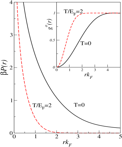
Figure 1: (Online color) The Ferm-hole potential (i.e., Pauli-exclusion potential) $\beta{\cal{P}}(r)$ is a universal function of $rk_{F}$ at each $T$ and reproduces the Fermi hole in the parallel-spin zeroth-order PDF, $g^{0}_{ss}(r)$, shown in the inset, for $T=0$ and $T/E_{F}=2$. If the spins are anti-parallel, $g^{0}_{s\neq s^{\prime}}(r)=1$ and the Pauli-exclusion potential is zero.

Assuming that $g^{0}_{ii}(r)$ can be modeled by an HNC fluid with the pair interaction $\beta{\cal{P}}(r)$, the “Fermi-hole potential”, viz., ${\cal{P}}(r)$, is easily seen to be given by

$$\beta{\cal{P}}(r)=-log[g^{0}(r)]+h^{0}(r)-c^{0}(r)$$ (10)

The $c^{0}(r)$ can be evaluated from $g^{0}_{T}(r)$ using the OZ relations. The $T=0$ case can be evaluated analytically lado .

We can determine only the product $\beta{\cal{P}}(r)$. The classical fluid “temperature” $1/\beta$ is still undefined and clearly cannot be the thermodynamic temperature $T$ as $T\to 0$. The Pauli-exclusion potential, i.e., the FHP, is a universal function of $rk_{F}$ at each $T$. It is long ranged and mimics the exclusion effects of Fermi statistics that produces quantum entanglement. At finite $T$ the range of the Pauli-exclusion potential is comparable to the de Broglie thermal wavelength and is increasingly hard-sphere like. Plots of $\beta{\cal{P}}(r)$ and $g^{0}_{ss}(r)$ are given in Fig. 1.

The next step in the CHNC method is to use the full pair-potential $\phi_{ij}(r)$, and solve the coupled HNC and OZ equations for the binary (up, and down spins) interacting  fluid. For the paramagnetic case, $\overline{n}_{i}$ = $\overline{n}/2$, we have:

$$g_{ij}(r) = e^{-\beta({\cal{P}}(r)\delta_{ij}+V_{cou}(r))+h_{ij}(r)-c_{ij}(r)}$$ (11)

$$h_{ij}(q) = \stackrel{{\scriptstyle FT}}{{\rightarrow}}h_{ij}(r)$$ (12)

$$h_{11}(q) = c_{11}(q)+(\overline{n}/2)[c_{11}(q)h_{11}(q)+c_{12}(q)h_{21}(q)]$$

$$h_{12}(q) = c_{12}(q)+(\overline{n}/2)[c_{11}(q)h_{12}(q)+c_{12}(q)h_{22}(q)]$$

The Coulomb potential $V_{cou}(r)$ needs some discussion. For two point-charge electrons this is $1/r$. However, depending on the temperature $T$, an electron is localized to within a thermal wavelength. Thus, following earlier work, e.g., Morita, and Minoo et al. minoo , we use a “diffraction-corrected” form:

$$V_{cou}(r)=(1/r)[1-e^{-r/\lambda_{th}}];\;\lambda_{th}=(2\pi\overline{m}T_{cf})^{-1/2}.$$ (14)

Here $\overline{m}$ is the reduced mass of the electron pair, i.e., $m^{*}(r_{s})/2$ a.u., where $m^{*}(r_{s})$ is the electron effective mass. It is weakly $r_{s}$ dependent, e.g, $\sim$0.96 for $r_{s}$ = 1. In this work we take $m^{*}$=1. The “diffraction correction” ensures the correct behaviour of $g_{12}(r\to 0)$ for all $r_{s}$.

In solving the above equations for a given $r_{s}$ and at $T$=0, we have $T_{cf}$=$T_{q}$. A trial $T_{q}$ is adjusted to obtain an $E_{c}(T_{q})$ equal to the known paramagnetic  $E_{c}(r_{s})$ at each $r_{s}$, via a coupling constant integration.

$$E_{xc}(T_{q})=\int_{0}^{1}\frac{d\lambda}{2}\int\frac{4\pi r^{2}dr}{r}[h_{11}(r,\lambda)+h_{12}(r,\lambda)]$$ (15)

($E_{x}$ alone is obtained if $\lambda$ is fixed at 0). The resulting “quantum” temperatures $T_{q}$ could be fitted to the form:

$$T_{q}/E_{F}=1.0/(a+b{\surd{r_{s}}}+cr_{s})$$ (16)

We have also presented a fit to the $T_{q}$ of the 2-D electron system, and discussed how the 2-D and 3-D fits could be related by a dimensional argument. Bulutay and Tanatar have also examined the CHNC method, and provided fits to the $T_{q}$ of the 2-D electron fluid bulutay .

For any given $r_{s}$, given the $T_{q}$ from the paramagnetic case, we can obtain $g_{ij}(r)$ and $E_{xc}(r_{s},\zeta,T)$ prl1 , at arbitrary  unexplored values of spin-polarization $\zeta$ by solving the coupled HNC equations, or doing an MD calculation using the Fermi-hole potential and the diffraction-corrected Coulomb potential. Many analytic theories of electron fluids, e.g., those of Singwi, Tosi, Land and Sjölander Mahan , Tanaka and Ichimaru, predict $g(r)$ which become negative for some values of $r$ even for moderate $r_{s}$. The PDFs obtained from the HNC-procedure are positive definite at all $r_{s}$. In Fig. 2 we show typical results for $g_{ij}(r)$ and comparisons with QMC-simulations. Our results are in excellent agreement with the DMC results prl1 .

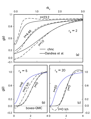
Figure 2: (Online colour) (a) The $g(r)$ from CHNC (solid lines) are compared with those of Dandrea et al. dun , (dashed lines) at $r_{s}$=2. The temperature $t=T/E_{F}$. Panel (b) $r_{s}=5$, CHNC (solid lines) for t=0 snd t=5. The $g(r)$ at $t=0$ from Tanaka and Ichimaru tan-ichi (dashed line), and from DMC-QMC ortiz94 (boxes), are also shown. Panel (c) $r_{s}=5$, CHNC (solid lines) for $t$=0 snd $t$=20. The $g(r)$ of Tanaka and Ichimaru tan-ichi (dashed line) is also shown for $t$=0.

The $T_{q}$ determined from the unpolarized $E_{c}$ is used to calculate $E_{c}(r_{s},\zeta,T)$ at any $\zeta$. The QMC results for $E_{c}(r_{s},\zeta)$ at $T=0$ agree with ours, since our $g_{ij}(r)$ agree with those from MC. For example, at $r_{s}$ = 10, the spin-polarized $-E_{c}$ is: Ceperley-Alder, 0.0209 Ry; Ortiz-Ballone, 0.0206 Ry ortiz94 ; our method (CHNC), 0.0201 Ry; Kallio and Piilo, 0.0171 Ry KP .

Most of the recent work using CHNC has been on the 2D-electron fluid owing to its accrued interest in nanostructures and technological applications. The electron-electrons interactions are stronger in reduced dimensions, and the use of a bridge function to supplement the CHNC equation is essential for accurate work br2d . However, even the appropriately chosen hard-disc bridge works quite well, as seen in Fig. 3.

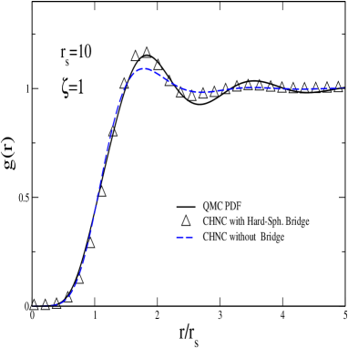
Figure 3: (Colour online)The QMC pair-distribution function of a fully spin polarized ($\zeta=1$) 2D electron fluid at $r_{s}=10$, and $T=0$ is compared with those calculated from CHNC using a hard-sphere bridge function and with no bridge function what so ever. An essentially exact fit with QMC can be obtained using a Coulomb bridge function br2d .

II.1 Fermi-liquid parameters of electron fluids

It is in fact possible that in some circumstances, WDM may fall into the category of a Fermi liquid. Highly compressed electron systems have correspondingly high Fermi energies and hence may have a physical temperature $T<<E_{F}$. In any case, we review the calculation of Fermi-liquid parameters as it is an important aspect of the capability of a classical map to extract results in the strong quantum domain.

Microscopic many-body physics allows one to calculate various quantities like the effective mass $m^{*}$ or the Landé $g$-factor that enter into Landau’s theory of Fermi liquids. One would perhaps assume that a classical representation of a Fermi liquid would hardly be successful in attacking such problems. For instance, $m^{*}$ is usually calculated from the solutions of the Dyson equation for the one-particle interacting Green’s function. If the real part of the retarded self-energy is $\Sigma_{1}(\vec{k},\omega)$, the Landau quasi-particle excitation energy $E_{QP}(\vec{k})$, measured with respect to the chemical potential is used in calculating the effective mass $m^{*}$.

$$E_{QP}(\vec{k}) = \epsilon_{k}+\Sigma_{1}(\vec{k},\omega)|_{\omega=E_{QP}}$$ (17)

$$\epsilon_{k} = k^{2}/2-E_{F}$$ (18)

$$\frac{1}{m^{*}} = \frac{dE_{QP}(k)}{k_{F}\,dk}|_{k=k_{F}}$$ (19)

This is a very arduous calculation, and there are technical questions about the difficulties of satisfying sum rules, Ward identities etc., when the Dyson equation is truncated in some approximation. The values of $m^{*}$ calculated by different authors using different perturbation expansions differ significantly, and from QMC results vigmstr05 ; quasi .

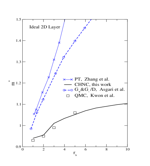
Figure 4: (Colour online) The effective mass $m^{*}$ of an ideal 2D layer (zero thickness) obtained from CHNC are compared with the the Quantum Monte Carlo data of Ref. kwon and the perturbation theory calculations of Zhang et al.zhang , and Asgari et al.vigmstr05 , i.e., their calculation labeled $G_{+}\&G_{-}/D$. The CHNC calculation is sensitive to the choice of the bridge function, while the Green’s-function methods are sensitive to the truncations used.

By contrast, the calculation of $m^{*}$, and also $g^{*}$ using CHNC is very simple because it can evaluate the free energy $F$ of the electron fluid as a function of the physical temperature $T$ as well as the spin polarization $\zeta$. The ratio of the interacting and non-interacting specific heats provides a simple evaluation of the $m^{*}$, while the ratio of the interacting and non-interacting susceptibilities, determined from the second derivative (with respect to $\zeta$) of the exchange-correlation correction to the free energy provides the product $m^{*}g^{*}$ quasi .

$$m^{*} = C_{v}/C_{v}^{0}=1+\frac{\left[\partial^{2}F_{xc}(t)/\partial t^{2}\right]}{\left[\partial^{2}F_{0}(t)/\partial t^{2}\right]}$$ (20)

$$(m^{*}g^{*})^{-1} = \chi_{P}/\chi_{s}=1+\frac{\left[\partial^{2}F_{xc}(\zeta)/\partial\zeta^{2}\right]}{\left[\partial^{2}F_{0}(\zeta)/\partial\zeta^{2}\right]}$$ (21)

Detailed calculations for ideal 2-D electron layers (see Fig. 4), thick layers as well as for multi-valley systems using the CHNC method have been presented in our publications quasi . Calculations of $m^{*}$ and $g^{*}$ for the 3-D electron liquid using CHNC have not yet been undertaken, while RPA results have been given by Rice Mahan .

III Dense Hydrogen and other plasmas

Dense hydrogen, or any other fully ionized plasma is a direct generalization of the uniform electron-fluid problem to include an additional component (e.g., protons), while removing the positive neutralizing background. Let us consider a fully ionized plasma with ions of charge $\overline{Z}$, and density $\rho$. Then the electron density $n=\overline{Z}\rho$, and we assume that both subsystems are at the same physical temperature $T$. The electron subsystem will have to be calculated at a classical-fluid temperature $T_{cf}=\surd(T_{q}^{2}+T^{2})$ and the electron-electron interactions have to be diffraction corrected. On the other hand, the ions are classical particles and the simulations (or integral equations) for the ions will use the physical temperature $T$. The quantum correction $T_{q}$ can be neglected for ion, as discussed in hyd . The total Hamiltonian now contains the three terms, $H_{i},H_{e}$, and the electron-ion interaction $H_{ei}$. The electron system contains two spin components, while the ion system adds another component. Thus, a three-component problem involving six pair-distribution functions have to be calculated. If spin effects could be neglected, then the two spin-components of the electrons could be replaced by an effective one-component electron fluid where the Pauli-exclusion potential (i.e, FHP) is included after averaging over the two components.

An example of a classical-map calculation of the EOS of laser-shock compressed hydrogen has been given by Dharma-wardana and Perrot hyd , where a Hugoniot has been calculated and compared with those from other methods (see Fig. 5). The article by Michael Desjarlais in this issue also refers to the problem of the equation of state (EOS) of highly compressed hydrogen Dejarlais11 . A proper experimental probe of such laser-compression experiments needs to address some method of independent measurement of the electron temperature $T_{e}$ and the ion temperature $T_{i}$. If the electrons and ions are in equilibrium, $T=T_{i}=T_{e}$. Then the usual DFT methods using the Born-Oppenheimer decoupling would be expected to give a good prediction of the EOS, and also the Hugoniot. The EOS calculation is essentially a calculation of the partition function. This requires the evaluation of

$$<e^{-(H_{e}/T_{e}+H_{i}/T_{i}+H_{ei}/T_{ei})}>$$ (22)

Here the total Hamiltonian $H$ is rewritten in terms of $H_{e}$, $H_{i}$, and the electron-ion interaction $H_{ei}$ which is again a Coulomb potential. We have included a cross-subsystem temperature $T_{ei}$ which is simply $T$ for equilibrium systems. If a Born-Oppenheimer approximation is used, the electrons ‘do not know’ the temperature of the ions, and vice versa. For equilibrium systems, a Born-Oppenheimer correction can be introduced, e.g., as in Morales et al. Morales10 . However, the add on correction introduced by Morales et al. will change the virial compressibility, leaving the small $k\to 0$ behaviour of the proton-proton structure factor unaffected, and hence the effect on the compressibility sum rules has to be examined. In any case the DFT implementations in codes like VASP, or SIESTA cannot deal correctly with the case $T_{i}\neq T_{e}$, and it is not clear if they treat the $H_{ei}$ term in the partition function correctly even in the equilibrium case, due to the use of the Born-Oppenheimer approximation which prevents the possibility of coupled electron-ion plasma modes in the system.

The CHNC technique is a non-dynamical method that does not need the Born-Oppenheimer approximation. It correctly treats the cross-interaction $H_{ei}$ even for two-temperature systems, as established by direct MD simulations cdw-mur . Fig. 5 shows that the SESEME and other standard EOS agree with the CHNC-BO calculation where $T_{ei}$ is set to $(T_{e}+T_{i})/2$, while the Laser-shock experiments, where $T_{i}\neq T_{e}$ may hold, should agree with $T_{ei}$ chosen as the temperature of the scattering pair. Ion masses are much larger than $m_{e}$, and hence $T_{ei}$ approaches the electron temperature, as demonstrated in Dharma-wardana and Murillo via MD simulations cdw-mur . In effect, the calculation of the Laser-shock hydrogen Hugoniot has to address non-equilibrium effects, as well as non-adiabatic effects associated with the use of the Born-Oppenheimer approximation in standard simulations. The conclusions of Galli et al. Galli02 also point to non-equilibrium effects associated with the electron-ion interaction, i.e., precisely the term $H_{ei}$ in the Hamiltonian indicated in Eq. 22. Our own views have evolved beyond what we stated in Ref. hyd , and the subject probably needs to be revisited, within a two-temperature quasi-equilibrium setting, without making the Born-Oppenheimer approximation, especially at very high compressions.

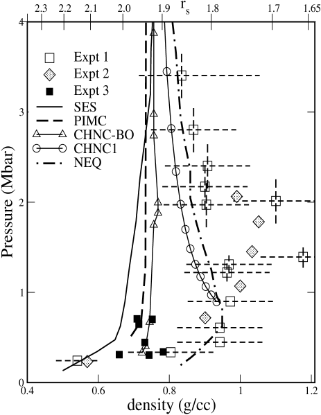
Figure 5: Comparison of the CHNC Hugoniot with experiment and other theories for warm-dense Deuterium. Of these, the SESEME (SES), path-integral Monte-Carlo (PIMC), CHNC-BO and the CHNC1 are of interest. A non-equilibrium Hugoniot, marked NEQ is also shown hyd . Experiments 1, 2 and 3 refer to Da Silva et al., Collins et al., and Knudson et al., respectively, as described in hyd .

III.1 Pseudopotentials

We may also consider the case when the ions are not fully ionized into bare nuclei, but carry a group of core electrons. For instance, Al-plasmas at 0.5 eV and normal compression have a charge $Z=3$ and a core of 10 electrons. Although it is sufficient for many problems to treat the Al³⁺ as point charges, a more accurate theory may wish to include the effect of the the core radius and well-depth of the electron-ion interaction via a pseudopotential. Such pseudopotentials are well known at zero temperature. A very simple model is that of Ashcroft, while modern implementations are very sophisticated.

Al-pseudopotentials suitable for WDM have been given in parametrized from by Perrot and Dharma-wardana elr98 . The basic idea is to generate the charge density $n(r)$ around a given nucleus of charge $Z_{N}$, immersed in a UEF of density parameter $r_{s}$, at a temperature $T$. The ion is place in a spherical cavity in the positive background (for details see Ref. elr98 ) and $n(r)$ is determined by a Kohn-Sham calculation which satisfies the Friedel sum rule and other properties. Then we define a weak non-local pseudopotential $V_{ps}(r)$ by the following relations in $q$-space.

$$V_{ps}(q,r_{s},T,Z_{N}) \equiv \Delta n(q,r_{s},T,Z_{N})/\chi(q,r_{s},T)$$ (23)

$$\chi(q) = \chi(q)^{0}/\{1-v_{q}(1-G_{q})\chi(q,r_{s},T)^{0}$$

Here $\chi^{0}(q,r_{s},T)$ is the Lindhard response function at finite $T$ and electron Wigner-Seitz radius $r_{s}$, $v_{q}=4\pi/q^{2}$ and $G_{q}$ is a local field correction consistent with the density and temperature of the UEF. Further more, $\Delta n(q,r_{s},T,Z_{N})$ is the Fourier transform of the real-space free-electron-density pileup $\Delta n(r)$ calculated at the jellium density $\overline{n}=3/(4\pi r_{s}^{3})$ and temperature $T$, for the nucleus $Z_{n}$. That is

$$\Delta n(r) = n_{f}(r)-\overline{n}$$ (24)

$$n_{f}(r) = n(r)-n_{b}(r)$$ (25)

The bound electron density $n_{b}(r)$ is obtained from the orbitals of the finite-$T$ Kohn-Sham equation as in Perrot Perrot93 . Here it should be noted that the bound electrons have to be assigned to a nucleus keeping in mind that some bound states are those of ‘hopping electrons’ which form a band of localized states near the continuum hopping92 . Equation 23 defines the pseudopotential to be capable of recovering the charge-pile up via linear response. Hence it has to render a weak potential. It is not very satisfactory if the resulting pseudopotential proves to be strong. However, the method seems to work in most cases. The pseudopotential can usually be parametrized (as in an Ashcroft empty-core potential), with a core depth $A_{0}$ and a core radius $r_{c}$ such that

$$V_{ps}(r) = -A_{0},\;\;r<r_{c}$$ (26)

$$= \overline{Z}/r,\;\;r>r_{c}$$ (27)

This is evidently a very simple form, compared to modern, hard, non-local pseudopotentials used in solid-state calculations at $T=0$. Such modern potentials remove the core, but a Kohn-Sham equation has to be solved as they are not weak, and cannot be treated using linear response. However, we have found that simple potentials as in Eqs. 23-26 are adequate for even the liquid-metal regime close to the melting point, even for metals which require non-local pseudopotentials at $T=0$. Excellent accuracy is obtained if the response functions $\chi(q)$ are calculated for electrons with an effective mass $m^{*}$ specified for each case. It is particularly important to note that the ‘mean ionization’, i.e., $\overline{Z}$ is a parameter which appears in the pseudopotential. The $\overline{Z}$ is also the Lagrange parameter defining the total charge neutrality of the plasma, as discussed in Refs. dwp82 , Perrot93 . A few examples of this type of simple pseudopotentials are given in Table 1.

Table 1: simple pseudopotentials for Al, C, Si at normal compression, and suitable for the WDM regime, in a.u.

element	$R_{WS}$	$\overline{Z}$	$A_{0}$	$r_{c}$	$m^{*}$
Al	3.141	3.0	0.3701	0.3054	0.998
C	2.718	4.0	0.0	0.3955	1.658
Si	3.073	4.0	0.0	0.9475	0.98

The C and Si pseudopotentials were used to generate PDFs of these ionic liquids and compared with Car-Parinello simulations in Ref. csige90 . Thus these pseudo-potentials can be used in the CHNC equations, or in the CMMD simulations, to take account of the existence of a finite-sized core. Such methods can be used to discuss properties of warm dense matter, thus providing a complementary approach to the simulations based on statistical potentials discussed by Graziani et al. in the context of the Cimarron project for simulations of warm dense matter Graziani11 .

IV Two-temperature quasi-equilibria and non-equilibrium systems.

When energy is deposited rapidly in matter using laser radiation, the electrons absorb the energy directly and equilibriate among themselves, achieving a very high electron temperature $T_{e}$. The ion subsystem, at temperature $T_{i}$, takes much longer to heat up due to the slow temperature relaxation via the electron-ion interaction. Hence, in laser-heated systems, it is common to find $T_{e}>T_{i}$. The inverse situation prevails in shock-heated materials since the energy of the shock wave couples to the heavy ions and not to the electrons Ng11 .

The possibility of using a static approach like the CHNC for non-equilibrium systems resides on Bogoliubov’s idea of timescales and conserved quantities. We have exploited these ideas in our work on hot-electron relaxation, both within Green’s-function methods, and within CHNC methods elr98 . The parameters $T_{e}$, $T_{i}$ in a two-temperature system are merely Lagrange parameters which assert that, for certain time scales $\tau_{e}$, $\tau_{i}$, the subsystem Hamiltonians $H_{e}$, $H_{i}$ are conserved quantities. Similarly, a number of other parameters, e.g., quasi-equilibrium chemical potentials, thermodynamic potentials, pseudopotentials, $\overline{Z}$, etc., attached to the subsystems may be conserved for the selected time scales. In fact, the original discussions of quasi-equilibria by Bogoluibov were used in Zubarev’s theory of non-equilibrium Green’s functions, and RPA-like results for the quasi-thermodynamics as well as energy relaxation were addressed there-in. However, RPA-like theories are of limited value. In strongly coupled regimes, the PDFs associated with the given subsystems can be constructed using CHNC, where the use of the correct inter-subsystem temperatures (e.g., $T_{ei}$) for evaluating inter-system PDFS (e.g., $g_{ei}$) is essential. The nature of this inter-system temperature is revealed by its appearance in the inter-subsystem energy-relaxation formula elr08 . A calculation of the distribution functions of two temperature plasmas using HNC methods as well as MD methods was given recently cdw-mur .

V Inhomogeneous systems

The classical-map technique uses a classical fluid at a finite temperature $T_{cf}$ to represent a uniform-density quantum fluid at $T=0$. The parameter $T_{cf}$ is density dependent, and hence the extension to a system with an inhomogeneous density is not straight-forward. Furthermore, integral-equation techniques like the HNC become very complicated when applied to inhomogeneous systems. Molecular dynamics can be applied if a viable mapping can be constructed. However in this connection we should note that studies of confined classical electrons in parabolic traps have also yielded useful insightsWrighton09 .

The classical-map technique treats the zeroth-order Hamiltonian exactly, i.e., the map is constructed to reproduce the known quantum solution classically, requiring the confining potential to be mapped as well. Even when there is no confining potential (other than a uniform background), the zeroth-order problem of $H^{0}$ has to be correctly treated. This was done in the UEF problem by constructing a Pauli exclusion potential (i.e., the Fermi-hole potential) to recover the Fermi hole in the $g^{0}_{ss}(r)$ exactly.

When non-interacting electrons are placed in an external potential, e.g., a parabolic trap, the uniform density $\overline{n}$ modifies to a new distribution $n^{0}(r)$. Classically, this distribution is of the Boltzmann form, Eq. 2 where $V_{KS}(r)$ contains all the terms found in the exponent of the HNC equation. Thus, given the $n^{0}(r)$ calculated from a quantum mechanical treatment of $H_{0}$ which contains the parabolic external potential, it is necessary to invert the HNC equation to get the effective classical potential which corresponds to $n^{0}(r)$. A simplified approach to this was used by us in ref. qdot09 . At this stage the calculation is somewhat similar to the determination of the Pauli exclusion potential, and hence the specification of an effective fluid temperature does not become necessary. The classical Coulomb fluid at a finite temperature $T_{cf}$ is still necessary for dealing with the many-body effects generated from the Coulomb interaction. However, given a non-uniform distribution, there is no evident method of defining a unique $T_{cf}$ and the simplicity of the original CHNC method is lost. Further more, the electron-electron pair-distribution functions now depend explicitly on two coordinates, viz., $g(\vec{r}_{1},\vec{r}_{2})_{ss^{\prime}}$. The use of molecular-dynamics simulations is more convenient in dealing with systems where the simplicity of homogeneous systems is lost. Another advantage an MD simulation is that the the bridge-function approximations are avoided.

In mapping an inhomogeneous system of density $n(r)$ to a homogeneous slab of density $\overline{n}$ we have used the form quasi ; Jost05 ; qdot09 ,

$$\overline{n}=<n(r)n(r)><n(r)>$$ (28)

in dealing with 2D systems. The same method has been used by Gori-Giorgi and Savin for 3D systems ggsavin . Using such a uniform density to define a unique temperature of an equivalent classical fluid, we were able to reproduce the charge distribution of interacting electrons in 2D quantum dots obtained from Quantum-Monte Carlo methods. However, as we used CHNC, it was necessary to introduce bridge-functions and boundary corrections which impaired the transparency of the classical map. Hence this work qdot09 may be regarded as a preliminary attempt.

VI Conclusion

We have outlined the classical-map technique of treating the quantum many-body problem in Fermi systems via a mapping to an equivalent classical system at a density-dependent effective temperature different from the physical temperature, and where the particles interact by a pair potential consisting of a Pauli-exclusion potential and a diffraction-corrected Coulomb potential. Large numbers of particles, and their thermodynamics or quasi-thermodynamics can be easily calculated. Since pair-distribution functions can be calculated accurately, and at any value of the coupling constant, the adiabatic connection formula provides results for the non-local exchange-correlation functionals in an entirely unambiguous, rigorous manner. No gradient corrections, meta-functionals etc., are needed. The Born-Oppenheimer approximation is not necessary as the CHNC technique is not dynamical. Hence the method would be of great interest from the point of view of equations-of-state studies, both for equilibrium, and for quasi-equilibrium systems.

Since suitable derivatives of the free energy with respect to density, temperature, and spin polarization lead to Landau Fermi-liquid parameters, the method is capable of easily furnishing alternative results for the effective mass $m^{*}$, Landé-$g$ factor, local-field factors of response functions etc., which are difficult to determine by standard Greens-function perturbation techniques of quantum many-body theory.

The application of the method to inhomogeneous systems is still poorly developed. Similarly, the method, being a technique for the total energy as a functional of the pair density, is similar to DFT in not yielding spectral information within its own formal structure.

References

- (1) Y. Ping, D. Hanson, I. Koslow, T. Ogitsu, D. Prendergast, E. Schwegler, G. Collins and Andew Ng. Phys. Rev. Lett. 96 255003 (2006)
- (2) Andre Ng, http://www.qtp.ufl.edu/sanibel/topics.shtml Sanibel Symposium. (2011)
- (3) P. Hohenberg and W. Kohn, Phys. Rev. 136, B864 (1964); D. Mermin, Phys. Rev. 137, A1441 (1965)
- (4) W. Kohn and L.J. Sham, Phys. Rev. 140, A1133 (1965)
- (5) F. Perrot, J. Phys.: Condens. matter 6, 431 (1994)
- (6) V.V. Karasiev, R.S. Jones, S.B. Trickey and Frank E. Harris, New developments in Quantum Chemistry, Eds. José Lous Paz, . J. Hernández, p25-54 (2009)
- (7) M.W.C. Dharma-wardana and F. Perrot, Phys. Rev. A 26, 2096 (1982)
- (8) T. L. Gilbert, Phys. Rev. B 12, 2111 (1975)
- (9) T. Kreibich and E.K.U. Gross. Phys. Rev. Lett., 86, 2984, (2001).
- (10) F. Lado, J. Chem. Phys. 47, 5369 (1967)
- (11) N. H. March, Phys. Lett. A 113 476 (1986)
- (12) S. B. Trickey, V. V. Karasiev, R. S. Jones, Int. J. Q. Chem. 109, 2951 (2009)
- (13) M. W. C. Dharma-wardana and F. Perrot, Phys. Rev. Lett. 84, 959 (2000)
- (14) F. Perrot and M.W.C. Dharma-wardana, Phys. Rev. B15 62, 16536 (2000) Erratum 67, 79901 (2003)
- (15) François Perrot and M. W. C. Dharma-wardana, Phys. Rev. Lett. 87, 206404 (2001)
- (16) C. Bulutay and B. Tanatar, Phys. Rev. B 65, 195116 (2002)
- (17) M. W. C. Dharma-wardana and F. Perrot, Phys. Rev. Lett. 90, 136601 (2003)
- (18) N. Q. Khanh and H. Totsuji, Solid State Com., 129, 37 (2004)
- (19) M. W. C. Dharma-wardana, Phys. Rev. B 72, 125339 (2005)
- (20) M. W. C. Dharma-wardana and F. Perrot., Europhys. lett. 63, 660 (2003)
- (21) M. W. C. Dharma-wardana and F. Perrot, Phys. Rev. B 70, 035308 (2004)
- (22) M. W. C. Dharma-wardana, Phys. Rev. B 75, 075427 (2007)
- (23) T. Miyake, C. Totsuji, K. Nakanishi, and H. Totsuji, Phys. Let. A 372, 6197 (2008).
- (24) M. W. C. Dharma-wardana , Physica E 41, 1285 (2009)
- (25) M. W. C. Dharma-wardana and M. S. Murillo, Phys. Rev. E. 77, 026401 (2008)
- (26) M. W. C. Dharma-wardana and F. Perrot, Phys. Rev. B, 66, 14110 (2002)
- (27) M. W. C. Dharma-wardana, Phys. Rev. E 73, 036401 (2006)
- (28) J. Chihara and S. Kambayashi, J. Phys: Condens. matter 6 10221 (1994)
- (29) Y. Rosenfeld and N.W. Ashcroft, Phys. Rev. A 20, 2162 (1979)
- (30) M. W. C. Dharma-wardana, Phys. Rev. B 82, 195303 (2010)
- (31) G. D. Mahan, Many-particle physics, Plenum Press, New York (1990)
- (32) M. Minoo, M. Gombert and C. Deutsch, Phys. Rev. A 23, 924 (1981)
- (33) R. B. Dandrea, N. W. Ashcroft and A. E. Carlsson, Phy. Rev. B 34, 2097 (1986).
- (34) S. Tanaka and S. Ichimaru, Phys. Rev. B 39, 1036 (1989)
- (35) G. Ortiz abd P. Ballone, Phys. Rev. B 50, 1391 (1994)
- (36) A. Kallio and J. Piilo, Phys. Rev. Lett. 77, 4237 (1996)
- (37) R. Asgari, B. Davoudi, M. Polini, M. P. Tosi, G. F. Giuliani, and G. Vignale, Phys. Rev. B 71, 45323 (2005).
- (38) Y. Kwon, D. M. Ceperley, and R. M. Martin, Phys. Rev. B 50, 1684 (1994)
- (39) Y. Zhang and S. Das Sarma, Phys. Rev. B 71,45322 (2005)
- (40) M. Desjarlais http://www.qtp.ufl.edu/sanibel/topics.shtml Sanibel Symposium. (2011)
- (41) Miguel A. Morales, Carlo Pierleoni, and D. M. Ceperley, Phys. Rev. B 81, 021202 (2010)
- (42) Giulia Galli, Randolph Q. Hood, Andrew U. Hazi, and François Gygi, Phys. Rev. B 61, 909 (2002); F. Gygi and G. Galli, 65. 220102 (2002)
- (43) F. Perrot, Phys. Rev. A 47 570 (1993); F. Perrot and M.W.C. Dharma-wardana, Phys. Rev. E. 52, 5352 (1995).
- (44) M.W.C. Dharma-wardana and F. Perrot, Phys. Rev. A 45,5883 (1992).
- (45) F. R. Graziani et al. Lawrence Livermore National Laboratory report, USA, LLNL-JRNL-469771 (2011)
- (46) M.W.C. Dharma-wardana and F. Perrot, Phys. Res. Lett. 65, 76 (1990)
- (47) M. W. C. Dharma-wardana, Phys. Rev. Lett. 101, 035002 (2008)
- (48) J. Wrighton, J. W. Dufty, H. Kählert and M. Bonitz, Phys. Rev. E 80, 066405 (2009)
- (49) M. W. C. Dharma-wardana and F. Perrot, Phys. Rev. E, 58, 3705 (1998);Errratum Phys. Rev. E 63, 069901 (2001)
- (50) D. Jost and M. W. C. Dharma-wardana, Phys. Rev. B, 72, 195315 (2005)
- (51) P. Gori-Giorgi and A. Savin, Phys. Rev. A 71 32513 (2005)