DOLFIN: Automated Finite Element Computing

Abstract

We describe here a library aimed at automating the solution of partial differential equations using the finite element method. By employing novel techniques for automated code generation, the library combines a high level of expressiveness with efficient computation. Finite element variational forms may be expressed in near mathematical notation, from which low-level code is automatically generated, compiled and seamlessly integrated with efficient implementations of computational meshes and high-performance linear algebra. Easy-to-use object-oriented interfaces to the library are provided in the form of a C++ library and a Python module. This paper discusses the mathematical abstractions and methods used in the design of the library and its implementation. A number of examples are presented to demonstrate the use of the library in application code.

A. Logg, Center for Biomedical Computing, Simula Research Laboratory, P.O. Box 134, 1325 Lysaker, Norway. Email: logg@simula.no.
G.N. Wells, Department of Engineering, University of Cambridge, Trumpington Street, Cambridge CB2 1PZ, United Kingdom. Email: gnw20@cam.ac.uk.

1 Introduction

Partial differential equations underpin many branches of science and their solution using computers is commonplace. Over time, the complexity and diversity of scientifically and industrially relevant differential equations has increased, which has placed new demands on the software used to solve them. Many specialized libraries have proved successful for a particular problem, but have lacked the flexibility to adapt to evolving demands.

Software for the solution of partial differential equations is typically developed with a strong focus on performance, and it is a common conception that high performance may only be obtained by specialization. However, recent developments in finite element code generation have shown that this is only true in part [Kirby et al. (2005), Kirby et al. (2006), Kirby and Logg (2006), Kirby and Logg (2007)]. Specialized code is still needed to achieve high performance, but the specialized code may be generated, thus relieving the programmer of time-consuming and error-prone tasks.

We present in this paper the library DOLFIN which is aimed at the automated solution of partial differential equations using the finite element method. As will be elaborated, DOLFIN relies on a form compiler to generate the innermost loops of the finite element algorithm. This allows DOLFIN to implement a general and efficient assembly algorithm. DOLFIN may assemble arbitrary rank tensors (scalars, vectors, matrices and higher-rank tensors) on simplex meshes in one, two and three space dimensions for a wide range of user-defined variational forms and for a wide range of finite elements. Furthermore, tensors may be assembled into any user-defined data structure, or any of the data structures implemented by one of the built-in linear algebra backends. For any combination of computational mesh, variational form, finite element and linear algebra backend, the assembly is performed by the same code, as illustrated schematically in Figure 1, and code generation allows the assembly code to be efficient and compact.

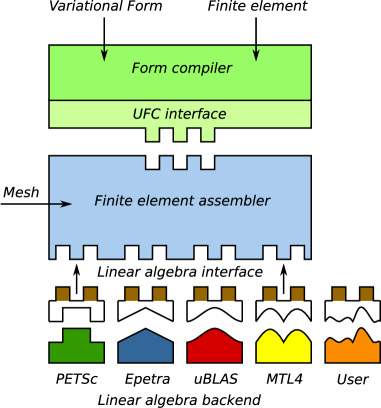
Figure 1: DOLFIN assembles any user-defined variational form on any (simplex) mesh for a wide range of finite elements using any user-defined or built-in linear algebra backend. DOLFIN relies on a form compiler for generation of the problem-specific code. The form compiler generates code conforming to the UFC (Unified Form-assembly Code) interface, either at compile-time or run-time, and the generated code is called during assembly by DOLFIN. A small interface layer is required for each linear algebra backend and is implemented as part of DOLFIN for PETSc, Trilinos/Epetra, uBLAS and MTL4.

DOLFIN functions as the main programming interface and problem solving environment of the FEniCS Project [FEniCS (2009)], a collaborative effort towards the development of innovative concepts and tools for the automation of computational mathematical modeling, with an emphasis on partial differential equations. See Logg2007a for a overview. All FEniCS components are released under the GNU General Public License or the GNU Lesser General Public License, and are made freely available at http://www.fenics.org.

Initially, DOLFIN was a monolithic, stand-alone C++ library including implementations of linear algebra, computational meshes, finite element basis functions, variational forms and finite element assembly. Since then, it has undergone a number of design iterations and some functionality has now been “outsourced” to other FEniCS components and third-party software. The design encompasses coexistence with other libraries, and permits a user to select particular components (classes) rather than to commit to a rigid framework or an entire package. The design also allows DOLFIN to provide a complex and feature-rich system from a relatively small amount of code, which is made possible through automation and design sophistication. For linear algebra functionality, third-party libraries are exploited, with a common programming interface to these backends implemented as part of DOLFIN. Finite element basis functions are evaluated by FIAT [Kirby (2009), Kirby (2004)] and variational forms are handled by the Unified Form Language (UFL) library [Alnæs and Logg (2009), Alnæs (2009)] and the FEniCS Form Compiler (FFC) [Logg et al. (2009), Kirby and Logg (2006)]. Alternatively, DOLFIN may use SyFi/SFC [Alnæs and Mardal (2009), Alnæs and Mardal (2010)] for these tasks, or any other form compiler that conforms to the Unified Form-assembly Code (UFC) interface [Alnæs et al. (2009)] for finite element code. Just-in-time compilation is handled by Instant [Alnæs et al. (2009)]. FIAT, FFC, SyFi/SFC, UFC and Instant are all components of the FEniCS Project. Data structures and algorithms for computational meshes remain implemented as part of DOLFIN, as is the general assembly algorithm.

Traditional object-oriented finite element libraries, including deal.II [Bangerth et al. (2007)] and Diffpack [Langtangen (2003)], provide basic tools such as computational meshes, linear algebra interfaces and finite element basis functions. This greatly simplifies the implementation of finite element methods, but the user must typically implement the assembly algorithm (or at least part of it), which is time-consuming and error-prone. There exist today a number of projects that seek to create systems that, at least in part, automate the finite element method, including Sundance [Long et al. (2009)], GetDP [Dular et al. (2009)], FreeFEM++ [Pironneau et al. (2009)] and Life [Prud’homme (2009), Prud’homme (2007)]. All of these rely on some form of preprocessing (compile-time or run-time) to allow a level of mathematical expressiveness to be combined with efficient run-time assembly of linear systems. DOLFIN differs from these project in that it relies more explicitly on code generation, which allows the assembly algorithms to be decoupled from the implementation of variational forms and finite elements. As a result, DOLFIN supports a wider range of finite elements than any of the above-mentioned libraries since it may assemble any finite element variational form on any finite element space supported by the form compiler and finite element backend.

The remainder of this paper is organized as follows. We first present a background to automated finite element computing in Section 2. We then present some general design considerations in Section 3 before discussing in more detail the design and implementation of DOLFIN in Section 4. We present in Section 5 a number of examples to illustrate the use of DOLFIN in application code, which is followed by concluding remarks in Section 6.

2 Automated Finite Element Computing

DOLFIN automates the assembly of linear and nonlinear systems arising from the finite element discretization of partial differential equations expressed in variational form. To illustrate this, consider the reaction–diffusion equation

$$-\Delta u+u=f$$ (1)

on the unit square $\Omega=(0,1)\times(0,1)$ with $f(x,y)=\sin(x)\cos(y)$ and homogeneous Neumann boundary conditions. The corresponding variational problem on $V=H^{1}(\Omega)$ reads:

$$\mbox{Find }u\in V:\quad a\left({v,u}\right)=L\left({v}\right)\quad\forall v\in V,$$ (2)

where

$$a(v,u) =\int_{\Omega}\nabla v\cdot\nabla u+vu\,\mathrm{d}x,$$ (3)

$$L(v) =\int_{\Omega}vf\,\mathrm{d}x.$$ (4)

To assemble and solve a linear system $AU=b$ for the degrees of freedom $U\in\mathbb{R}^{N}$ of a finite element approximation $u_{h}=\sum_{i=1}^{N}U_{i}\phi_{i}\in V_{h}\subset V$, where the set of basis functions $\left\{{\phi_{i}}\right\}_{i=1}^{N}$ spans $V_{h}$, one may simply define the bilinear (3) and linear (4) forms, and then call the two functions assemble and solve in DOLFIN. This is illustrated in Table 1 where we list a complete program for solving the reaction–diffusion problem (1) using piecewise linear elements.

Python code  

from dolfin import *

mesh = UnitSquare(32, 32)
V = FunctionSpace(mesh, "CG", 1)

v = TestFunction(V)
u = TrialFunction(V)
f = Expression("sin(x[0])*cos(x[1])")

A = assemble(dot(grad(v), grad(u))*dx + v*u*dx)
b = assemble(v*f*dx)

u_h = Function(V)
solve(A, u_h.vector(), b)

plot(u_h)

 

Table 1: A complete program for solving the reaction–diffusion problem (1) and plotting the solution. This and other presented code examples are written for DOLFIN version 0.9.5 (released in December 2009).

The example given in Table 1 illustrates the use of DOLFIN for solving a particularly simple equation, but assembling and solving linear systems remain the two key steps in the solution of more complex problems. We return to this in Section 5.

2.1 Automated code generation

DOLFIN may assemble a variational form of any rank from a large class of variational forms and it does so efficiently by automated code generation. Following a traditional paradigm, it is difficult to build automated systems that are at the same time general and efficient. Through automated code generation, one may build a system which is both general and efficient.

DOLFIN relies on a form compiler to automatically generate code for the innermost loop of the assembly algorithm from a high-level mathematical description of a finite element variational form, as discussed in kirby:2006 and oelgaard:2008. As demonstrated in kirby:2006, computer code can be generated which outperforms the usual hand-written code for a class of problems by using representations which can not reasonably be implemented by hand. Furthermore, automated optimization strategies can be employed [Kirby et al. (2005), Kirby et al. (2006), Kirby and Logg (2007), Ølgaard and Wells (2010)] and different representations can be used, with the most efficient representation depending on the nature of the differential equation [Ølgaard and Wells (2010)]. Recently, similar results have been demonstrated in SyFi/SFC [Alnæs and Mardal (2010)].

Code generation adds an extra layer of complexity to a software system. For this reason, it is essential to isolate the parts of a program for which code must be generated. The remaining parts may be implemented as reusable library components in a general purpose language. Such library components include data structures and algorithms for linear algebra (matrices, vectors and linear/nonlinear solvers), computational meshes, representation of functions, input/output and plotting. However, the assembly of a linear system from a given finite element variational formulation must be implemented differently for each particular formulation and for each particular choice of finite element function space(s). In particular, the innermost loop of the assembly algorithm varies for each particular problem. DOLFIN follows a strategy of re-usable components at higher levels, but relies on a form compiler to generate the code for the innermost loop from a user-defined high-level description of the finite element variational form.

DOLFIN partitions the user input into two subsets: data that may only be handled efficiently by special purpose code, and data that can be efficiently handled by general purpose library components. For a typical finite element application, the first set of data may consist of a finite element variational problem and the finite element(s) used to define it. The second set of data consists of the mesh and possibly other parameters that define the problem. The first set of data is given to a form compiler that generates special purpose code. That special purpose code may then use the second set of data as input to compute the solution. If the form compiler is implemented as a just-in-time (JIT) compiler, one may seamlessly integrate the code generation into a problem solving environment to automatically generate, compile and execute generated code at run-time on demand. We present this process schematically in Figure 2.

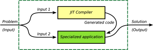
Figure 2: An automated system (DOLFIN) using a JIT compiler to generate special purpose code for a subset of its input. For a typical finite element application, Input 1 consists of the variational problem and the finite element(s) used to define it, and Input 2 consists of the mesh.

2.2 Compilation of variational forms

Users of DOLFIN may use one of the two form compilers FFC or SyFi/SFC to generate problem-specific code. When writing a C++ application based on DOLFIN, the form compiler must be called explicitly from the command-line prior to compile-time. The form compiler generates C++ code which may be included in a user program. The generated code defines a number of classes that may be instantiated by the user and passed to the DOLFIN C++ library. In particular, the user may instantiate form objects which correspond to the variational forms given to the form compiler and which may be passed as input arguments to the assembly function in DOLFIN. When using DOLFIN from Python, DOLFIN automatically handles the communication with the form compiler, the compilation (and caching) of the generated code and the instantiation of the generated form classes at run-time (JIT compilation).

3 Design Considerations

The development of DOLFIN has been driven by two keys factors. The first is striving for technical innovation. Examples of this include the use of a form compiler to generate code and new data structures for efficient representation of computational meshes [Logg (2009)]. A second driving force is provided by the needs of applications; diverse and challenging applications have demanded and resulted in generic solutions for broad classes of problems. Often the canonical examples have not exposed limitations in the technology, particularly with respect to how the time required for code generation scales with the complexity of the considered equation [Ølgaard and Wells (2010)]. These have only become evident and then addressed when attempting to solve challenging problems at the limits of current technology. It is our experience that both these components are necessary to drive advances and promote innovation. We comment in this section on some generic design considerations that have been important in the development of DOLFIN.

3.1 Languages and language features

DOLFIN is written primarily in C++ with interfaces provided both in the form of a C++ class library and a Python module. The bulk of the Python interface is generated automatically using SWIG [SWIG (2009), Beazley (2003)], with some extensions hand-written in Python. The Python interface offers the performance of the underlying C++ library with the ease of an intuitive scripting language. Performance critical operations are developed in C++, and users can develop solvers based on DOLFIN using either the C++ or Python interface.

A number of C++ libraries for finite element analysis make extensive use of templates. Templated classes afford considerable flexibility and can be particularly useful in combining high-level abstractions and code re-use with performance as they avoid the cost inherent in virtual function calls in C++. However, the extensive use of templates can obfuscate code, it increases compilation times and compiler generated error messages are usually expansive and difficult to interpret. We use templates in DOLFIN where performance demands it, and where it enables reuse of code. However, a number of key operations in a finite element library which require a function call involve a non-trivial number of operations within the function, and in these cases we make use of traditional C++ polymorphism. This enhances readability and simplifies debugging compared to template-based solutions, while not affecting run-time performance since the extra cost of a virtual function call is negligible compared to, for example, computing an element matrix or inserting the entries of an element matrix into a global sparse matrix. At the highest levels of abstraction, users are exposed to very few templated classes and objects, which simplifies the syntax of user-developed solvers. The limited use of templates at the user level also simplifies the automated generation of the DOLFIN Python interface.

In mirroring mathematical concepts in the library design, sharing of data between objects has proved important. For example, objects representing functions may share a common object representing a function space, and different function spaces may share a common object representing a mesh. We have dealt with this issue through the use of shared pointers, and in particular boost::shared_ptr from Boost. In managing data sharing, this solution has reduced the complexity of classes and improved the robustness of the library. While we make use of shared pointers, they are generally transparent to the user and need not be used in the high-level interface, thereby not burdening a user with the more complicated syntax.

3.2 Interfaces

Many scientific libraries perform a limited number of specialized operations which permits exposing users to a minimal, high-level interface. DOLFIN provides such a high-level interface for solving partial differential equations, which in many cases allows non-trivial problems to be solved with less than 20 lines of code (as we will demonstrate in Section 5). At the same time, it is recognized that methods for solving partial differential equations are diverse and evolving. Therefore, DOLFIN provides interfaces of varying complexity levels. For some problems, the minimal high-level interface will suffice, whereas other problems may be solved using a mixture of high- and low-level interfaces. In particular, users may often rely on the DOLFIN Function class to store and hide the degrees of freedom of a finite element function. Nevertheless, the degrees of freedom of a function may still be manipulated directly if desired.

The high-level interface of DOLFIN is based on a small number of classes representing common mathematical abstractions. These include the classes Matrix, Vector, Mesh, FunctionSpace, Function and VariationalProblem. In addition to these classes, DOLFIN provides a small number of free functions, including assemble, solve and plot. We discuss these classes and functions in more detail in Section 4.

DOLFIN relies on external libraries for a number of important tasks, including the solution of linear systems. In cases where functionality provided by external libraries must be exposed to the user, simplified wrappers are provided. This way, DOLFIN preserves a consistent user interface, while allowing different external libraries which perform similar tasks to be seamlessly interchanged. It also permits DOLFIN to set sensible default options for libraries with complex interfaces that require a large number of parameters to be set. This is most evident in the use of libraries for linear algebra. While the simplified wrappers defined by DOLFIN are usually sufficient, access is permitted to the underlying wrapped objects so that advanced users may operate directly on those objects when necessary.

4 Design and Implementation

Like many other finite element libraries, DOLFIN is designed as a collection of classes partitioned into components/libraries of related classes. However, while these classes are typically implemented as part of the library, see, e.g., bangerth:2007, DOLFIN relies on automated code generation and external libraries for the implementation of a large part of the functionality. Figure 3 shows a UML diagram of the central components and classes of DOLFIN. These include the linear algebra classes, mesh classes, finite element classes and function classes. As already touched upon above, the linear algebra classes consist mostly of wrapper classes for external libraries. The finite element classes Form, FiniteElement and DofMap are also wrapper classes but for generated code, whereas the classes Assembler, VariationalProblem together with the mesh and function classes are implemented as regular C++ classes (with Python wrappers) as part of DOLFIN. In the following, we address these key components of DOLFIN, in order of increasing abstraction. In addition to the components depicted in Figure 3, DOLFIN includes a number of additional components for input/output, logging, plotting and the solution of ordinary differential equations.

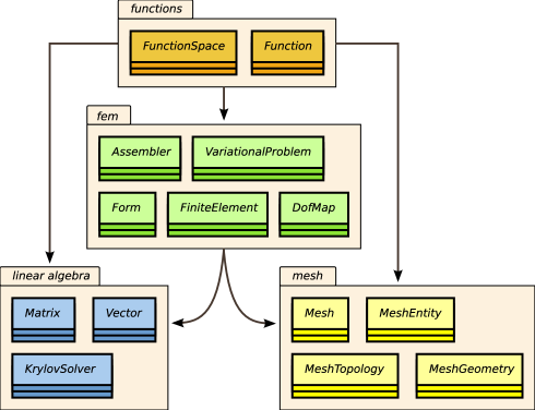
Figure 3: UML diagram of the central components and classes of DOLFIN.

4.1 Linear algebra

DOLFIN allows the transparent use of various specialized linear algebra libraries. This includes the use of data structures for sparse and dense matrices, preconditioners and iterative solvers, and direct linear solvers. This approach allows users to leverage the particular strengths of different libraries through a simple and uniform interface. Currently supported linear algebra backends include PETSc [Balay et al. (2009)], Trilinos/Epetra [Heroux et al. (2005)], uBLAS [Walter et al. (2009)] and MTL4 [Gottschling and Lumsdaine (2009)]. Interfaces to the direct solvers UMFPACK [Davis (2004)] (sparse LU decomposition) and CHOLMOD [Chen et al. (2008)] (sparse Cholesky decomposition) are also provided.

The implementation of the DOLFIN linear algebra interface is based on C++ polymorphism. A common abstract base class GenericMatrix defines a minimal matrix interface suitable for finite element assembly, and a subclass of GenericMatrix implements the functionality for each backend by suitably wrapping native data structures of its respective backend. Similarly, a common abstract base class GenericVector defines a minimal interface for vectors with subclasses for all backends. The two interface classes GenericMatrix and GenericVector are themselves subclasses of a common base class GenericTensor. This enables DOLFIN to implement a common assembly algorithm for all matrices, vectors and scalars (or any other rank tensor) for all linear algebra backends. Compared to a template-based solution, polymorphism may incur overhead associated with the cost of resolving virtual function calls. However, the most performance-critical function call to the linear algebra backend during assembly is typically insertion of a local element matrix into a global sparse matrix. This operation usually involves a considerable amount of computation/memory access, hence the extra cost of the virtual function call in this case may be neglected. For cases in which the overhead of a virtual function call is not negligible, operating directly on the underlying object avoids this overhead.

4.2 Meshes

The DOLFIN Mesh class is based on a simple abstraction that allows dimension-independence, both in the implementation of the DOLFIN mesh library and in user code. In particular, the DOLFIN assembly algorithm is common for all simplex meshes in one, two and three space dimensions. We provide here an overview of the DOLFIN mesh implementation and refer to logg:2008 for details. While only simplices are currently supported, the design paradigm extends to non-simplicial meshes.

A DOLFIN mesh consists of a collection of mesh entities that define the topology of the mesh, together with a geometric mapping embedding the mesh entities in $\mathbb{R}^{n}$. A mesh entity is a pair $(d,i)$, where $d$ is the topological dimension of the mesh entity and $i$ is a unique index of the mesh entity. A similar approach may be found in KnepleyKarpeev07A. Mesh entities are numbered within each topological dimension from $0$ to $n_{d}-1$, where $n_{d}$ is the number of mesh entities of topological dimension $d$. For convenience, mesh entities of topological dimension $0$ are referred to as vertices, entities of dimension $1$ edges, entities of dimension $2$ faces, entities of codimension $1$ facets and entities of codimension $0$ cells. These concepts are summarized in Table 2.

Entity	Class	Dimension	Codimension
Mesh entity	MeshEntity	$d$	$D-d$
Vertex	Vertex	$0$	$D$
Edge	Edge	$1$	$D-1$
Face	Face	$2$	$D-2$
Facet	Facet	$D-1$	$1$
Cell	Cell	$D$	$0$

Table 2: DOLFIN mesh abstractions and corresponding classes. Users may refer to a mesh entity either by a topological dimension and index or as a named mesh entity such as a vertex with a specific index.

Algorithms operating on a mesh can often be expressed in terms of iterators [Berti (2002), Berti (2006)]. The mesh library provides the general iterator MeshEntityIterator in addition to the specialized mesh iterators VertexIterator, EdgeIterator, FaceIterator, FacetIterator and CellIterator. We illustrate the use of iterators in Table 3.

C++ code  

Mesh mesh("mesh.xml");

for (CellIterator cell(mesh); !cell.end(); ++cell)
  for (VertexIterator vertex(*cell); !vertex.end(); ++vertex)
      cout << vertex->dim() << " " << vertex->index() << endl;
    

 

Python code  

mesh = Mesh("mesh.xml")

for cell in cells(mesh):
    for vertex in vertices(cell):
        print vertex.dim(), vertex.index()
    

 

Table 3: Basic use of DOLFIN mesh iterators for iterating over all vertices of all cells of a mesh in C++ (top) and Python (bottom).

The DOLFIN mesh library also introduces the concept of a mesh function. A mesh function, and its corresponding implementation MeshFunction, is a discrete function on the set of mesh entities of a specific dimension. It is only defined on a set of mesh entities which is in contrast to functions represented by the DOLFIN Function class which take a value at each point in the domain covered by the mesh. The class MeshFunction is templated over the value type which allows users, for example, to create a boolean-valued mesh function over the cells of a mesh to indicate regions for mesh refinement, an integer-valued mesh function on vertices to indicate a mapping from local to global vertex numbers or a float-valued mesh function on cells to indicate material data.

The simple object-oriented interface of the DOLFIN mesh library is combined with efficient storage of the underlying mesh data structures. Objects like vertices, edges and faces are never stored. Instead, DOLFIN stores all mesh data in plain C/C++ arrays and provides views of the underlying data in the form of the class MeshEntity and its subclasses Vertex, Edge, Face, Facet and Cell, together with their corresponding iterator classes. An earlier version of the DOLFIN mesh library used a full object-oriented model also for storage, but the simple array-based approach has reduced storage requirements and improved the speed of accessing mesh data by orders of magnitude [Logg (2009)]. In its initial state, the DOLFIN Mesh class only stores vertex coordinates, using a single array of double values, and cell–vertex connectivity, using a compressed row-like data structure consisting of two arrays of unsigned int values. Any other connectivity, such as, vertex–vertex, edge–cell or cell–facet connectivity, is automatically generated and stored when required. Thus, if a user solves a partial differential equation using piecewise linear elements on a tetrahedral mesh, only cell-vertex connectivity is required and so edges and faces are not generated. However, if quadratic elements are used, edges are automatically generated and cubic elements will lead to a generation of faces as well as edges.

In addition to efficient representation of mesh data, the DOLFIN mesh library implements a number of algorithms which operate on meshes, including adaptive mesh refinement (using a rivara:1991-type method), mesh coarsening and mesh smoothing. DOLFIN does not provide support for mesh generation, except for a number of simple shapes like squares, boxes and spheres. The following code illustrates adaptive mesh refinement in DOLFIN: C++ code  

MeshFunction<bool> cell_markers(mesh, mesh.topology().dim());

for (CellIterator cell(mesh); !cell.end(); ++cell)
{
  if (...)
    cell_markers[*cell] = true;
  else
    cell_markers[*cell] = false;
}

mesh.refine(cell_markers);
mesh.smooth();

 

4.3 Finite elements

DOLFIN supports a wide range of finite elements. At present, the following elements are supported:

1. $H^{1}$-conforming finite elements:

   1. $\mathrm{CG}_{q}$, arbitrary degree continuous Lagrange elements.

2. $H(\mathrm{div})$-conforming finite elements:

   1. $\mathrm{RT}_{q}$, arbitrary degree Raviart–Thomas elements [Raviart and Thomas (1977)];

   2. $\mathrm{BDM}_{q}$, arbitrary degree Brezzi–Douglas–Marini elements [Brezzi et al. (1985)]; and

   3. $\mathrm{BDFM}_{q}$, arbitrary degree Brezzi–Douglas–Fortin–Marini elements [Brezzi et al. (1987)].

3. $H(\mathrm{curl})$-conforming finite elements:

   1. $\mathrm{NED}_{q}$, arbitrary degree Nédélec elements (first kind) [Nédélec (1980)].

4. $L^{2}$-conforming finite elements:

   1. $\mathrm{DG}_{q}$, arbitrary degree discontinuous Lagrange elements; and

   2. $\mathrm{CR}_{1}$, first degree Crouzeix–Raviart elements [Crouzeix and Raviart (1973)].

Arbitrary combinations of the above elements may be used to define mixed elements. Thus, one may for example define a Taylor–Hood element by combining a vector-valued $P_{2}$ element with a scalar $P_{1}$ element. Arbitrary nesting is supported, thus allowing a mixed Taylor–Hood element to be used as a building block in a coupled problem which involves more than just the velocity and pressure fields. In Section 5, we demonstrate the use of mixed elements for the Poisson equation. Presently, DOLFIN only supports elements defined on simplices. This is not a technical limitation in the library design, but rather a reflection of current user demand.

DOLFIN relies on a form compiler such as FFC for the implementation of finite elements. FFC in turn relies on FIAT for tabulation of finite element basis functions on a reference element. In particular, for any given element family and degree $q$ from the list of supported elements, FFC generates C++ code conforming to a common interface specification for finite elements which is part of the UFC interface. Thus, DOLFIN does not include a library of finite elements, but relies on automated code generation, either prior to compile-time or at run-time, for the implementation of finite elements. The generated code may be used for efficient run-time evaluation of finite element basis functions, derivatives of basis functions and evaluation of degrees of freedom (applying the functionals to any given function). However, these functions are rarely accessed by users as a user is not usually exposed to the details of a finite element beyond its declaration, and since DOLFIN automates the assembly of variational forms based on code generation for evaluation of the element matrix. Detailed aspects of automated finite element code generation can be found in oelgaard:2008 for discontinuous elements and in rognes:2008 for $H({\rm div})$ and $H({\rm curl})$ elements.

4.4 Function spaces

The concept of a function space plays a central role in the mathematical formulation of finite element methods for partial differential equations. DOLFIN mirrors this concept in the class FunctionSpace. This class defines a finite dimensional function space in terms of a Mesh, a FiniteElement and a DofMap (degree of freedom map): C++ code  

class FunctionSpace
{
public:
  ...
private:
  ...
  boost::shared_ptr<const Mesh> _mesh;
  boost::shared_ptr<const FiniteElement> _element;
  boost::shared_ptr<const DofMap> _dofmap;
};

 
The mesh defines the domain, the finite element defines the local basis on each cell and the degree of freedom map defines how local function spaces are patched together to form the global function space.

For some problems, finite element spaces are not appropriate and a “quadrature function space” can be used. In such a “space”, functions can be evaluated at discrete points (quadrature points) but not elsewhere, and derivatives cannot be computed. This concept is discussed in oelgaard:2008 and oelgaard:2009.

Incorporating the mathematical concept of function spaces in the library design provides a powerful abstraction, especially for sharing data in a transparent and simple fashion. In particular, several functions may share the same function space and thus the same mesh, finite element and degree of freedom mapping.

4.5 Functions

Functions on a finite element function space are implemented in DOLFIN in the form of the Function class. A Function is expressed as a linear combination of basis functions on a discrete finite element or quadrature space. The expansion coefficients (degrees of freedom) of the Function are stored as a (Generic)Vector: C++ code  

class Function
{
public:
  ...
private:
  ...
  boost::shared_ptr<const FunctionSpace> _function_space;
  boost::shared_ptr<GenericVector> _vector;
};

 

A Function may be evaluated at arbitrary points on a finite element mesh, used as a coefficient in a variational form, saved to file for later visualization or plotted directly from within DOLFIN. The DOLFIN Function class is particularly powerful for supplying and exchanging data between different models in coupled problems, as will be demonstrated in Section 5.

Evaluation of Functions at arbitrary points is handled efficiently using the GNU Triangulated Surface Library [GTS (2009)]. With the help of GTS, DOLFIN locates which cell of the Mesh of the FunctionSpace contains the given point. The function value may then be computed by evaluating the finite element basis functions at the given point (using the FiniteElement of the FunctionSpace) and multiplying with the appropriate coefficients in the Vector (determined using the DofMap of the FunctionSpace).

4.6 Expressions

Many times, it is appropriate to express a coefficient in a variational problem by an expression or an algorithm for evaluating the coefficient at a given point, rather than expressing it as a linear combination of basis functions (as in the Function class). Such coefficients may be conveniently implemented using the Expression class.

An Expression is defined by a user through overloading the Expression::eval function. This functor construct provides a powerful mechanism for defining complex coefficients. In particular, the functor construct allows a user to attach data to an Expression. A user may, for example, read data from a file in the constructor of an Expression subclass which is then later accessed in the eval callback function.

For the definition of functions given by simple expressions, like $f(x)=\sin(x)$ or $g(x,y)=\sin(x)\cos(y)$, the DOLFIN Python interface provides simple and automated JIT compilation of expressions. While the Python interface does allow a user to overload the eval function from Python, this may be inefficient as the call to eval involves a callback from C++ to a Python function and this may be called repeatedly during assembly (once or more on each cell). However, JIT compilation avoids this by automatically generating, compiling, wrapping and linking C++ subclasses of the Expression class.

An Expression may be evaluated at arbitrary points on a finite element mesh, used as a coefficient in a variational form, projected or interpolated into a finite element function space or plotted directly from within DOLFIN. Table 4 illustrates use of the DOLFIN Function and Expression classes in Python.

Python code  

# Create mesh
mesh = UnitSquare(32, 32)

# Define an expression
f = Expression(("sin(x[0])", "cos(x[1])"))

# Project expression to a finite element space
V = VectorFunctionSpace(mesh, "CG", 2)
g = project(f, V)

# Evaluate expression and function
print f(0.1, 0.2)
print g(0.1, 0.2)

# Plot expression and function
plot(f, mesh=mesh)
plot(g)
    

 

Table 4: Defining, projecting, evaluating and plotting expressions and functions using the DOLFIN Python interface.

4.7 Variational forms

DOLFIN allows general variational forms to be expressed in a form language that mimics mathematical notation. For example, consider the bilinear form of the standard Stokes variational problem. This may be conveniently expressed in the form language as illustrated in Table 5.

Mathematical notation

$a(v,u)=\int_{\Omega}\operatorname{grad}v\cdot\operatorname{grad}u-\operatorname{div}v\,p+q\,\operatorname{div}u\,\mathrm{d}x$

Code

a = (inner(grad(v), grad(u)) - div(v)*p + q*div(u))*dx

Table 5: Expressing the bilinear form for the Stokes equations in DOLFIN.

The form language allows the expression of general multilinear forms of arity $\rho$ on the product space $V_{h}^{1}\times V_{h}^{2}\times\cdots\times V_{h}^{\rho}$ of a sequence $\{V_{h}^{j}\}_{j=1}^{\rho}$ of finite element spaces on a domain $\Omega\subset\mathbb{R}^{n}$,

$$a:V_{h}^{1}\times V_{h}^{2}\times\dots\times V_{h}^{\rho}\rightarrow\mathbb{R}.$$ (5)

Such forms are fundamental building blocks in linear and nonlinear finite element analysis. In particular, linear forms ($\rho=1$) and bilinear forms ($\rho=2$) are central to the finite element discretization of partial differential equations. Forms of higher arity are also supported as they may sometimes be of interest, see kirby:2006.

DOLFIN relies on the Unified Form Language (UFL) [Alnæs and Logg (2009), Alnæs (2009)] for the expression of variational forms. The form language allows the expression of a wide range of finite element variational forms in a language close to mathematical notation. UFL also supports functional differentiation of general nonlinear forms. Forms can involve integrals over cells, interior facets and exterior facets. Line and surface integrals which do not coincide with cell facets are not yet supported, although extensions in this direction for modeling crack propagation have been made [Nikbakht and Wells (2009)]. For details on the form language, we refer to the UFL user manual [Alnæs and Logg (2009)].

A user of the DOLFIN C++ interface will typically define a set of forms in one or more form files and call FFC on the command-line. The generated code may then be included in the user’s C++ program. As an illustration, consider again the bilinear form of the Stokes problem as expressed in Table 5. This may be entered together with the corresponding linear form L = v*f*dx in a text file named Stokes.ufl which may then be compiled with FFC:

ffc -l dolfin Stokes.ufl

This will generate a C++ header file Stokes.h which a user may include in a C++ program to instantiate the pair of forms: C++ code  

#include <dolfin.h>
#include "Stokes.h"
...
int main()
{
  ...
  Stokes::FunctionSpace V(mesh);
  Stokes::BilinearForm a(V, V);
  Stokes::LinearForm L(V);
  ...
}

 
When used from Python, form compilation is handled automatically by DOLFIN. If a form is encountered during the execution of a program, the necessary C++ code is automatically generated and compiled. The generated object code is cached so that code is generated and compiled only when necessary. Thus, if a user solves the Stokes problem twice, code is only generated the first time, as the JIT compiler will recognize the Stokes form on subsequent runs.

4.8 Finite element assembly

Given a variational form, the DOLFIN assemble function assembles the corresponding global tensor. In particular, a matrix is assembled from a bilinear form, a vector is assembled from a linear form, and a scalar value is assembled from a rank zero form (a functional). While DOLFIN does not provide data structures for sparse tensors of rank greater than two, the abstract GenericTensor interface, which was introduced in Section 4.1, permits users to supply data structures for arbitrary rank tensors.

To discretize the multilinear form (5), we may introduce a basis $\{\phi^{j}_{k}\}_{k=1}^{N_{j}}$ for each function space $V^{j}_{h}$, $j=1,2,\ldots,\rho$, and define the global tensor

$$A_{i}=a(\phi_{i_{1}}^{1},\phi_{i_{2}}^{2},\dots,\phi_{i_{\rho}}^{\rho}),$$ (6)

where $i=(i_{1},i_{2},\dots,i_{\rho})$ is a multi-index. If the multilinear form is defined as an integral over $\Omega=\cup_{K\in\mathcal{T}_{h}}K$, the tensor $A$ may be computed by assembling the contributions from all elements,

$$A_{i}=a(\phi_{i_{1}}^{1},\phi_{i_{2}}^{2},\dots,\phi_{i_{\rho}}^{\rho})=\sum_{K\in\mathcal{T}}a^{K}(\phi_{i_{1}}^{1},\phi_{i_{2}}^{2},\dots,\phi_{i_{\rho}}^{\rho}),$$ (7)

where $a^{K}$ denotes the contribution from element $K$. We further let $\{\phi_{k}^{K,j}\}_{k=1}^{n_{j}}$ denote the local finite element basis for $V^{j}_{h}$ on $K$ and define the element tensor $A^{K}$ (the “element stiffness matrix”) by

$$A_{i}^{K}=a^{K}(\phi_{i_{1}}^{K,1},\phi_{i_{2}}^{K,2},\dots,\phi_{i_{\rho}}^{K,\rho}).$$ (8)

The assembly of the global tensor $A$ thus reduces to the computation of the element tensor $A^{K}$ on each element $K$ and the insertion of the entries of $A^{K}$ into the global tensor $A$. In addition to contributions from all cells, DOLFIN also assembles contributions from all exterior facets (facets on the boundary) and all interior facets if required.

The key to the generality and efficiency of the DOLFIN assembly algorithm lies in the automated generation of code for the evaluation of the element tensor. DOLFIN relies on generated code both for the evaluation of the element tensor and the mapping of degrees of freedom. Thus, the assembly algorithm may call the generated code on each cell of the mesh, first to compute the element tensor and then again to compute the local-to-global mapping by which the entries of the element tensor may be inserted into the global tensor. The complexity inherent in non-trivial forms, such as those which involve mixed element spaces, vector elements and discontinuous Galerkin methods, is not exposed in the form abstraction. DOLFIN is unaware of how the element matrix is represented or how forms are integrated. It simply provides coefficient and mesh data to the generated code and assembles the computed results. The algorithm for computing the element tensor is instead determined by the form compiler. Various algorithms are possible, including both quadrature and a special tensor representation, and the most efficient algorithm can depend heavily on the nature of the form [Kirby and Logg (2006), Ølgaard and Wells (2010)].

To assemble a Form a, a user may simply call the function assemble which computes and returns the corresponding tensor. Thus, a bilinear form may be assembled by C++ code  

  Matrix A;
  assemble(A, a);

 
in C++ and Python code  

  A = assemble(a)

 
in Python. Several optional parameters may be given to specify either assembly over specific subdomains of the mesh or reuse of tensors.

4.9 Boundary conditions

Natural boundary conditions are enforced weakly as part of a variational problem and are typically of Neumann or Robin type, but may also be of Dirichlet type as will be demonstrated Section 5. Essential boundary conditions are typically of Dirichlet type and are enforced strongly at the linear algebra level. DOLFIN also supports the specification of periodic boundary conditions. We describe here the definition and application of strong Dirichlet boundary conditions.

We define a Dirichlet boundary condition in terms of a function space $V$, a function $g$ and a subset of the boundary $\Gamma\subseteq\partial\Omega$,

$$u(x)=g(x)\quad\forall x\in\Gamma.$$ (9)

The corresponding definition in the DOLFIN Python interface reads Python code  

bc = DirichletBC(V, g, gamma)

 
where V is a FunctionSpace, g is a Function or Expression, and gamma is a SubDomain. Alternatively, the boundary may be defined in terms of a MeshFunction marking a portion of the facets on the mesh boundary. The function space V defines the space to which the boundary condition will be applied. This is useful when applying a Dirichlet boundary condition to particular components of a mixed or vector-valued problem.

Once a boundary condition has been defined, it can be applied in one of two ways. The simplest is to act upon the assembled global system: Python code  

bc.apply(A, b)

 
For each degree of freedom to be constrained, this call will zero the corresponding row in the matrix, set the diagonal entry to one and put the Dirichlet value at the corresponding position in the right-hand side vector. An optional argument can be provided for updating the boundary conditions inside a Newton iteration. Alternatively, the boundary condition may be supplied directly to the assembler which will then apply the boundary condition by modifying the element matrices in a manner that preserves any symmetry of the global matrix: Python code  

A, b = assemble_system(a, L, bc)

 

4.10 Variational problems

At the highest level of abstraction, objects may be created that represent variational problems of the canonical form (2). Such a variational problem may be defined and solved by Python code  

problem = VariationalProblem(a, L)
u = problem.solve()

 
A constraint on the trial space in the form of one or more Dirichlet conditions may be supplied as additional arguments. Other parameters include the specification of the linear solver and preconditioner (when appropriate) and whether or not the variational problem is linear. In the case of a nonlinear variational problem where one seeks to satisfy

$$F(v)=0\quad\forall\ v\in V,$$ (10)

the bilinear form $a$ is interpreted as the Gateaux derivative of a nonlinear form $L=F$.

4.11 File I/O and visualization

DOLFIN provides input/output for objects of all its central container classes, including Vector, Matrix, Mesh and MeshFunction. Objects are stored to file in XML format. For example, a Mesh may be loaded from and stored back to file by C++ code  

File file("mesh.xml");
Mesh mesh;

file >> mesh;
file << mesh;

 
Mesh data may be converted to the native DOLFIN XML format from Gmsh, Medit, Diffpack, ABAQUS, Exodus II and StarCD formats using the conversion utility dolfin-convert.

Solution data may be exported in a number of formats, including the VTK XML format which is useful for visualizing a Function in VTK-based tools, such as ParaView. DOLFIN also provides built-in plotting for Mesh, MeshFunction and Function using Viper [Skavhaug (2009)] by C++ code  

plot(mesh);
plot(mesh_function);
plot(u);

 

5 Applications

We present here a collection of examples to demonstrate the use of DOLFIN for solving partial differential equations and related problems of interest. A more extensive range of examples are distributed with the DOLFIN source code. For a particularly complicated application to reservoir modeling, we refer to wells:2009. Some issues of particular relevance to solid mechanics problems, such as plasticity, are discussed in oelgaard:2008c. All examples correspond to DOLFIN 0.9.5.

5.1 Evaluating functionals

We begin with the simplest form that we can evaluate, a functional. In the absence of viscous stresses, the lift acting on a body can be computed by integrating the pressure multiplied by a suitable component of the unit vector normal to the surface of interest. The definition of this functional is shown in Table 6. From this definition, C++ code may be generated using a form compiler and then used to compute the lift generated by a computed pressure field.

Form compiler code  

element = FiniteElement("Lagrange", triangle, 1)

p = Function(element)
n = triangle.n
M = p*n[1]*ds

 

Table 6: Definition of the functional for computing the lift.

Another common application of functionals is the evaluation of various norms or evaluating the error of a computed solution when the exact solution is known. For example, one may define the squared $L^{2}$ and $H^{1}_{0}$ norms as v*v*dx and dot(grad(v), grad(v))*dx respectively. Alternatively, one may use the built-in DOLFIN functions norm and errornorm to evaluate norms and errors: Python code  

print norm(v, "L2")
print norm(v, "H1")
print norm(v, "H10")
print norm(v, "Hdiv")
...
print errornorm(u_h, u, "L2")
print errornorm(u_h, u, "H1")
print errornorm(u_h, u, "H10")
print errornorm(u_h, u, "Hdiv")
...

 

5.2 Solving linear partial differential equations

To illustrate the use of DOLFIN for solving simple linear partial differential equations, we consider Poisson’s equation $-\Delta u=f$ discretized using three different methods: an $H^{1}$-conforming primal approach using standard continuous Lagrange basis functions; a mixed method using $H(\operatorname{div})\times L^{2}$-conforming elements; and a discontinuous Galerkin method using $L^{2}$-conforming Lagrange basis functions.

5.2.1 $H^{1}$-conforming discretization of Poisson’s equation

For the standard $H^{1}$-conforming approach, the bilinear and linear forms are given by

$$a(v,u) =\int_{\Omega}\nabla v\cdot\nabla u\,\mathrm{d}x,$$ (11)

$$L(v) =\int_{\Omega}vf\,\mathrm{d}x,$$ (12)

and the forms may be specified in DOLFIN by Python code  

V = FunctionSpace(mesh, "CG", 1)
v = TestFunction(V)
u = TrialFunction(V)
f = Expression(...)

a = dot(grad(v), grad(u))*dx
L = v*f*dx

 

5.2.2 $H(\operatorname{div})\times L^{2}$-conforming discretization of Poisson’s equation

For the mixed version of the Poisson problem, with $u=0\ {\rm on}\ \partial\Omega$, the bilinear and linear forms read [Brezzi and Fortin (1991)]:

$$a(\tau,w;\sigma,u) =\int_{\Omega}\tau\cdot\sigma-(\nabla\cdot\tau)\,u+w\,(\nabla\cdot\sigma)\,\mathrm{d}x,$$ (13)

$$L(\tau,w) =\int_{\Omega}wf\,\mathrm{d}x,$$ (14)

where $\tau,\sigma\in V$, $w,u\in W$ and

$$V =\left\{{\tau\in H\left({{\rm div},\Omega}\right):\tau|_{K}\in[P_{q}]^{n}\left({K}\right)\,\forall K}\right\},$$ (15)

$$W =\left\{{w\in L^{2}\left({\Omega}\right):w|_{K}\in P_{q-1}\left({K}\right)\,\forall K}\right\}.$$ (16)

The corresponding implementation in DOLFIN for $q=2$ reads:

Python code  

V = FunctionSpace(mesh, "BDM", 2)
W = FunctionSpace(mesh, "DG", 1)

mixed_space = V + W

(tau, w)   = TestFunctions(mixed_space)
(sigma, u) = TrialFunctions(mixed_space)

f = Expression(...)

a = (dot(tau, sigma) - div(tau)*u + w*div(sigma))*dx
L = w*f*dx

 

5.2.3 $L^{2}$-conforming discretization of Poisson’s equation

For a discontinuous interior penalty formulation of the Poisson problem, the bilinear and linear forms read:

$$a(v,u)=\int_{\Omega\backslash\Gamma^{0}}\nabla v\cdot\nabla u\,\mathrm{d}x-\int_{\Gamma^{0}}\llbracket{v}\rrbracket\cdot\langle{\nabla u}\rangle\,\mathrm{d}s-\int_{\Gamma^{0}}\langle{\nabla v}\rangle\cdot\llbracket{u}\rrbracket\,\mathrm{d}s\\ -\int_{\partial\Omega}v\boldsymbol{n}\cdot\nabla u\,\mathrm{d}s-\int_{\partial\Omega}\nabla v\cdot u\boldsymbol{n}\,\mathrm{d}s+\int_{\Gamma^{0}}\frac{\alpha}{h}\llbracket{v}\rrbracket\cdot\llbracket{u}\rrbracket\,\mathrm{d}s+\int_{\partial\Omega}\frac{\alpha}{h}vu\,\mathrm{d}s$$ (17)

and

$$L(v)=\int_{\Omega}vf\,\mathrm{d}x,$$ (18)

where $\Gamma^{0}$ denotes all interior facets and $v,u\in V=\left\{{v\in L^{2}\left({\Omega}\right):v|_{K}\in P_{q}\left({K}\right)\,\forall K}\right\}$. Using ds to denote integration over exterior facets and dS to denote integration over interior facets, the corresponding implementation in DOLFIN for $q=1$ reads as follows: Python code  

V = FunctionSpace(mesh, "DG", 1)

v = TestFunction(V)
u = TrialFunction(V)
f = Expression(...)

n = FacetNormal(mesh)
h = CellSize(mesh)

alpha = 4.0

a =   dot(grad(v), grad(u))*dx \
    - dot(jump(v, n), avg(grad(u)))*dS \
    - dot(avg(grad(v)), jump(u, n))*dS \
    - v*dot(grad(u), n)*ds - dot(grad(v), n)*u*ds \
    + alpha/h(’+’)*dot(jump(v, n), jump(u, n))*dS \
    + (alpha/h)*v*u*ds

L = v*f*dx

 

5.3 Solving time-dependent partial differential equations

Unsteady problems can be solved by defining a variational problem to be solved in each time step. We illustrate this by solving the convection–diffusion problem

$$\dot{u}+b\cdot\nabla u-\nabla\cdot(c\nabla u)=f.$$ (19)

The velocity field $b=b(x)$ may be a user-defined expression or an earlier computed solution. Multiplying (19) with a test function and discretizing in time using the Crank–Nicolson method, we obtain

$$\int_{\Omega}v\,(u^{n}-u^{n-1})+k_{n}\,v\,\bar{b}\cdot\nabla\bar{u}+k_{n}\,\bar{c}\nabla v\cdot\nabla\bar{u}\,\mathrm{d}x=\int_{\Omega}k_{n}\,v\bar{f}\,\mathrm{d}x,$$ (20)

where $k_{n}=t_{n}-t_{n-1}$ is the time step and $\bar{x}=(x^{n}+x^{n-1})/2$. We may implement the problem (20) in DOLFIN by moving all terms involving $u^{n-1}$ to the right-hand side. Alternatively, we may rely on the built-in operators lhs and rhs to extract the pair of bilinear and linear forms as illustrated in Table 7. In Table 8 we show the corresponding C++ program.

Form compiler code  

scalar = FiniteElement("Lagrange", triangle, 1)
vector = VectorElement("Lagrange", triangle, 2)

v  = TestFunction(scalar)  # test function
u1 = TrialFunction(scalar) # solution at t_n
u0 = Function(scalar)      # solution at t_{n-1}
b  = Function(vector)      # convective velocity
f  = Function(scalar)      # source term
c  = 0.005                 # diffusivity
k  = 0.05                  # time step

u = 0.5*(u0 + u1)
F = v*(u1 - u0)*dx + k*v*dot(b, grad(u))*dx + k*c*dot(grad(v), grad(u))*dx
a = lhs(F)
L = rhs(F) + k*v*f*dx

 

Table 7: Specification of the variational problem for the unsteady convection-diffusion equation (19).

C++ code  

// Read mesh from file
Mesh mesh("mesh.xml.gz");

// Read velocity field from file
Velocity::FunctionSpace W(mesh);
Function velocity(W, "velocity.xml.gz");

// Read sub domain markers from file
MeshFunction<unsigned int> sub_domains(mesh, "subdomains.xml.gz");

// Create function space
ConvectionDiffusion::FunctionSpace V(mesh);

// Create source term and initial condition
Constant f(0);
Function u(V);

// Set up variational forms
ConvectionDiffusion::BilinearForm a(V, V);
a.b = velocity;
ConvectionDiffusion::LinearForm L(V);
L.u0 = u; L.b = velocity; L.f = f;

// Set up boundary condition
Constant g(1);
DirichletBC bc(V, g, sub_domains, 1);

// Linear system
Matrix A;
Vector b;

// Assemble matrix and apply boundary conditions
assemble(A, a);
bc.apply(A);

// Parameters for time-stepping
double T = 2.0; double k = 0.05; double t = k;

// Output file
File file("temperature.pvd");

// Time-stepping
while (t < T)
{
  assemble(b, L);
  bc.apply(b);
  solve(A, u.vector(), b, lu);
  file << u;
  t += k;
}

 

Table 8: Implementation of the solver for the unsteady convection-diffusion equation (19).

5.4 Solving nonlinear partial differential equations

Solution procedures for nonlinear differential equations are inherently more complex and diverse than those for linear equations. With this in mind, the design of DOLFIN allows users to build complex solution algorithms for nonlinear problems using the basic building blocks assemble and solve. However, a built-in Newton solver is also provided which suffices for many problems. We illustrate the solution of a nonlinear problem for the following nonlinear Poisson-like equation:

$$-\nabla\cdot\left({1+u^{2}}\right)\nabla u =f\quad\mbox{ in }\Omega,$$ (21)

$$u =0\quad\mbox{ on }\partial\Omega.$$ (22)

Multiplying by a test function $v\in V=H^{1}_{0}(\Omega)$ and integrating over the domain $\Omega$, we obtain

$$F(v;u)\equiv\int_{\Omega}\left({1+u^{2}}\right)\nabla v\cdot\nabla u\,\mathrm{d}x-\int_{\Omega}vf=0,$$ (23)

where we note that $F:V\times V\rightarrow\mathbb{R}$ is linear in its first argument and nonlinear in its second argument. To solve the nonlinear problem by Newton’s method, we compute the Gateaux derivative $D_{u}F(v;u)$ and obtain

$$\begin{split}a(v,\delta u;u)&\equiv D_{u}F(v;u)\delta u=\left.\frac{dF(v;u+\epsilon\delta u)}{d\epsilon}\right|_{\epsilon=0}\\ &=\int_{\Omega}\left({1+u^{2}}\right)\nabla v\cdot\nabla\delta u\,\mathrm{d}x+\int_{\Omega}2u\delta u\nabla v\cdot\nabla u\,\mathrm{d}x.\end{split}$$ (24)

We note that $F(\cdot;u):V\rightarrow\mathbb{R}$ is a linear form for every fixed $u$ and that $a(\cdot,\cdot;u):V\times V\rightarrow\mathbb{R}$ is a bilinear form for every fixed $u$. A full solver for (21)–(22) in the case $f(x,y)=x\sin y$ is presented in Table 9. The form language UFL supports automatic differentiation, so many problems, including this one, can also be linearized automatically.

Python code  

from dolfin import *

# Create mesh and define function space
mesh = UnitSquare(32, 32)
V = FunctionSpace(mesh, "CG", 1)

# Define boundary condition
bc = DirichletBC(V, Constant(0), DomainBoundary())

# Define source term and solution function
f = Expression("x[0]*sin(x[1])")
u = Function(V)

# Define variational problem
v  = TestFunction(V)
du = TrialFunction(V)
a  = (1.0 + u*u)*dot(grad(v), grad(du))*dx + \
     2*u*du*dot(grad(v), grad(u))*dx
L  = (1.0 + u*u)*dot(grad(v), grad(u))*dx - v*f*dx

# Solve nonlinear variational problem
problem = VariationalProblem(a, L, bc, nonlinear=True)
problem.solve(u)

# Plot solution and solution gradient
plot(u)
plot(grad(u))

 

Table 9: Implementation of a solver for the nonlinear Poisson problem (21)–(22).

6 Conclusions

We have presented a problem solving environment that largely automates the finite element approximation of solutions to differential equations. This is achieved by generating computer code for parts of the problem which are specific to the considered differential equation, and designing a generic library which reflects the mathematical structure of finite element variational problems. Using a high level of mathematical abstraction and automated code generation, the system can be designed for both readability and performance, allowing new models to be implemented rapidly and solved efficiently.

Until recently, the focus has been on automating the assembly of linear systems arising from the finite element discretization of variational problems, in particular with regards to providing a general implementation independent of the variational problem, the mesh, the discretizing finite element space(s) and the linear algebra backend. More recently, efficient parallel computing has been added and automated error estimation/adaptivity is being developed. We acknowledge the contributions that many people have made to the development of DOLFIN. Johan Hoffman and Johan Jansson both contributed to early versions of DOLFIN, in particular with algorithms for adaptive mesh refinement and solution of ordinary differential equations. Martin Alnæs, Kent-Andre Mardal and Ola Skavhaug have been involved in the design and implementation of the DOLFIN linear algebra interfaces and backends. Johan Hake and Ola Skavhaug have made significant contributions to the design of the DOLFIN Python interface. Johannes Ring and Ilmar Wilbers maintain the DOLFIN build system and produce packages for various platforms. We also mention Benjamin Kehlet, Gustav Magnus Vikstrøm, Kristian Ølgaard, Niclas Jansson, Dag Lindbo, Åsmund Ødegard, Evan Lezar and Shawn Walker.

AL is supported by an Outstanding Young Investigator grant from the Research Council of Norway, NFR 180450.

received

References

- Alnæs (2009) Alnæs, M. S. 2009. A compiler framework for automatic linearization and efficient discretization of nonlinear partial differential equations. Ph.D. thesis, University of Oslo. http://simula.no/research/sc/publications/Simula.SC.626/simula_pdf_file%.
- Alnæs et al. (2009) Alnæs, M. S., Langtangen, H. P., Logg, A., Mardal, K.-A., and Skavhaug, O. 2009. UFC. http://www.fenics.org/wiki/UFC/.
- Alnæs and Logg (2009) Alnæs, M. S. and Logg, A. 2009. UFL. http://www.fenics.org/wiki/UFL/.
- Alnæs and Mardal (2009) Alnæs, M. S. and Mardal, K.-A. 2009. SyFi. http://www.fenics.org/wiki/SyFi/.
- Alnæs and Mardal (2010) Alnæs, M. S. and Mardal, K.-A. 2010. On the efficiency of symbolic computations combined with code generation for finite element methods. ACM Transactions on Mathematical Software 37, 6:1–6:26.
- Alnæs et al. (2009) Alnæs, M. S., Mardal, K.-A., and Westlie, M. 2009. Instant. http://www.fenics.org/wiki/Instant.
- Balay et al. (2009) Balay, S., Buschelman, K., Gropp, W. D., Kaushik, D., Knepley, M. G., McInnes, L. C., Smith, B. F., and Zhang, H. 2009. PETSc Web page. http://www.mcs.anl.gov/petsc/.
- Bangerth et al. (2007) Bangerth, W., Hartmann, R., and Kanschat, G. 2007. deal.II — A general purpose object oriented finite element library. ACM Transactions on Mathematical Software 33, 4, 24.
- Beazley (2003) Beazley, D. M. 2003. Automated scientific software scripting with SWIG. Future Generation Computer Systems 19, 5, 599–609.
- Berti (2002) Berti, G. 2002. Generic programming for mesh algorithms: Towards universally usable geometric components. In Proceedings of the Fifth World Congress on Computational Mechanics (WCCM V), H. A. Mang, F. G. Rammerstorfer, and J. Eberhardsteiner, Eds. Vienna University of Technology, Vienna. http://wccm.tuwien.ac.at/publications/Papers/fp81327.pdf.
- Berti (2006) Berti, G. 2006. GrAL – The grid algorithms library. Future Generation Computer Systems 22.
- Brezzi et al. (1987) Brezzi, F., Douglas, Jr., J., Fortin, M., and Marini, L. D. 1987. Efficient rectangular mixed finite elements in two and three space variables. RAIRO – Analyse Numerique – Numerical Analysis 21, 4, 581–604.
- Brezzi et al. (1985) Brezzi, F., Douglas, Jr., J., and Marini, L. D. 1985. Two families of mixed finite elements for second order elliptic problems. Numerische Mathematik 47, 2, 217–235.
- Brezzi and Fortin (1991) Brezzi, F. and Fortin, M. 1991. Mixed and Hybrid Finite Element Methods. Springer Series in Computational Mathematics, vol. 15. Springer, New York.
- Chen et al. (2008) Chen, Y., Davis, T. A., Hager, W. W., and Rajamanickam, S. 2008. Algorithm 887: CHOLMOD, supernodal sparse Cholesky factorization and update/downdate. ACM Transactions on Mathematical Software 35, 3, 1–14.
- Crouzeix and Raviart (1973) Crouzeix, M. and Raviart, P. A. 1973. Conforming and nonconforming finite element methods for solving the stationary stokes equations. RAIRO – Analyse Numerique – Numerical Analysis 7, 33–76.
- Davis (2004) Davis, T. A. 2004. Algorithm 832: UMFPACK v4.3—an unsymmetric-pattern multifrontal method. ACM Transactions on Mathematical Software 30, 2, 196–199.
- Dular et al. (2009) Dular, P., Geuzaine, C., et al. 2009. GetDP: A general environment for the treatment of discrete problems. http://geuz.org/getdp/.
- FEniCS (2009) FEniCS. 2009. FEniCS Project. http://www.fenics.org/.
- Gottschling and Lumsdaine (2009) Gottschling, P. and Lumsdaine, A. 2009. The Matrix Template Library 4. http://www.osl.iu.edu/research/mtl/mtl4/.
- GTS (2009) GTS 2009. GNU Triangulated Surface Library (GTS). http://gts.sourceforge.net/.
- Heroux et al. (2005) Heroux, M. A., Bartlett, R. A., Howle, V. E., Hoekstra, R. J., Hu, J. J., Kolda, T. G., Lehoucq, R. B., Long, K. R., Pawlowski, R. P., Phipps, E. T., Salinger, A. G., Thornquist, H. K., Tuminaro, R. S., Willenbring, J. M., Williams, A., and Stanley, K. S. 2005. An overview of the Trilinos project. ACM Transactions on Mathematical Software 31, 3, 397–423.
- Kirby (2004) Kirby, R. C. 2004. Algorithm 839: FIAT, a new paradigm for computing finite element basis functions. ACM Transactions on Mathematical Software 30, 4, 502–516.
- Kirby (2009) Kirby, R. C. 2009. FIAT. http://www.fenics.org/fiat/.
- Kirby et al. (2005) Kirby, R. C., Knepley, M. G., Logg, A., and Scott, L. R. 2005. Optimizing the evaluation of finite element matrices. SIAM Journal on Scientific Computing 27, 3, 741–758.
- Kirby and Logg (2006) Kirby, R. C. and Logg, A. 2006. A compiler for variational forms. ACM Transactions on Mathematical Software 32, 3, 417–444.
- Kirby and Logg (2007) Kirby, R. C. and Logg, A. 2007. Efficient compilation of a class of variational forms. ACM Transactions on Mathematical Software 33, 3.
- Kirby et al. (2006) Kirby, R. C., Logg, A., Scott, L. R., and Terrel, A. R. 2006. Topological optimization of the evaluation of finite element matrices. SIAM Journal on Scientific Computing 28, 1, 224–240.
- Knepley and Karpeev (2009) Knepley, M. G. and Karpeev, D. A. 2009. Mesh algorithms for PDE with Sieve I: Mesh distribution. Scientific Programming 17, 3, 215–230.
- Langtangen (2003) Langtangen, H. P. 2003. Computational Partial Differential Equations: Numerical Methods and Diffpack Programming. Texts in Computational Science and Engineering, vol. 1. Springer.
- Logg (2007) Logg, A. 2007. Automating the finite element method. Arch. Comput. Methods Eng. 14, 2, 93–138.
- Logg (2009) Logg, A. 2009. Efficient representation of computational meshes. International Journal of Computational Science and Engineering 4, 4, 283–295.
- Logg et al. (2009) Logg, A., Ølgaard, K. B., Rognes, M. E., Wells, G. N., et al. 2009. FFC. http://www.fenics.org/ffc/.
- Long et al. (2009) Long, K. et al. 2009. Sundance. http://www.math.ttu.edu/~klong/Sundance/html/.
- Nédélec (1980) Nédélec, J.-C. 1980. Mixed finite elements in . Numerische Mathematik 35, 3, 315–341.
- Nikbakht and Wells (2009) Nikbakht, M. and Wells, G. N. 2009. Automated modelling of evolving discontinuities. Algorithms 2, 3, 1008–1030.
- Ølgaard et al. (2008) Ølgaard, K. B., Logg, A., and Wells, G. N. 2008. Automated code generation for discontinuous Galerkin methods. SIAM Journal on Scientific Computing 31, 2, 849–864.
- Ølgaard and Wells (2010) Ølgaard, K. B. and Wells, G. N. 2010. Optimisations for quadrature representations of finite element tensors through automated code generation. ACM Transactions on Mathematical Software 37, 1, 8:1–8:23.
- Ølgaard et al. (2008) Ølgaard, K. B., Wells, G. N., and Logg, A. 2008. Automated computational modelling for solid mechanics. In IUTAM Symposium on Theoretical, Computational and Modelling Aspects of Inelastic Media, B. D. Reddy, Ed. IUTAM Bookseries, vol. 11. Springer, 195–204.
- Pironneau et al. (2009) Pironneau, O., Hecht, F., and Le Hyaric, A. 2009. FreeFEM++. http://www.freefem.org/.
- Prud’homme (2007) Prud’homme, C. 2007. Life: Overview of a unified C++ implementation of the finite and spectral element methods in 1D, 2D and 3D. In Applied Parallel Computing. State of the Art in Scientific Computing. Lecture Notes in Computer Science, vol. 4699/2009. Springer Berlin / Heidelberg, 712–721.
- Prud’homme (2009) Prud’homme, C. 2009. Life. http://ljkforge.imag.fr/life.
- Raviart and Thomas (1977) Raviart, P.-A. and Thomas, J. M. 1977. Primal hybrid finite element methods for nd order elliptic equations. Mathematics of Computation 31, 138, 391–413.
- Rivara (1991) Rivara, M.-C. 1991. Local modification of meshes for adaptive and/or multigrid finite-element methods. Journal of Computational and Applied Mathematics 36, 1, 79 – 89.
- Rognes et al. (2009) Rognes, M. E., Kirby, R. C., and Logg, A. 2009. Efficient assembly of and conforming finite elements. SIAM Journal on Scientific Computing 31, 6, 4130–4151.
- Skavhaug (2009) Skavhaug, O. 2009. Viper. http://www.fenics.org/wiki/Viper.
- SWIG (2009) SWIG 2009. Simplified Wrapper and Interface Generator (SWIG). http://www.swig.org/.
- Walter et al. (2009) Walter, J., Koch, M., et al. 2009. uBLAS. http://www.boost.org/.
- Wells et al. (2008) Wells, G. N., Hooijkaas, T., and Shan, X. 2008. Modelling temperature effects on multiphase flow through porous media. Philosophical Magazine 88, 28–29, 3265–3279.