Ionized bubble number count as a probe of non-Gaussianity

Abstract

The number count of ionized bubbles on a map of 21 cm fluctuations with the primordial non-Gaussianity is investigated. The existence of the primordial non-Gaussianity modifies the reionization process, because the formation of collapsed objects, which could be the source of reionization photons, is affected by the primordial non-Gaussianity. In this paper, the abundance of ionized bubbles is calculated by using a simple analytic model with the local type of the primordial non-Gaussianity, which is parameterized by $f_{NL}$. In order to take into account the dependence of the number count on the size of ionized bubbles and the resolution of the observation instrument, a threshold parameter $B_{b}$ which is related to the the surface brightness temperature contrast of an ionized bubble is introduced. We show the potential to put the constraint on $f_{NL}$ from the number count by future observations such as LOFAR and SKA.

1 introduction

Recent cosmic microwave background (CMB) observations have revealed the statistical nature of primordial fluctuations and given the strong support of the inflationary scenario (Komatsu et al., 2009). However, it is still difficult to specify the model among the inflationary scenario from CMB observations. The measurement (or even the upper bound) of non-Gaussianity of primordial fluctuations is, on the other hand, expected to have the potential to rule out many inflationary models. Although the primordial fluctuations are predicted as nearly Gaussian in all inflationary models, the degree of the deviation from the Gaussianity depends on each specific model. The slow-roll inflation models with a single scalar field produce almost pure Gaussian fluctuations (Guth & Pi, 1982; Starobinsky, 1982; Bardeen et al., 1983), and the deviation from the Gaussianity is unobservably small (Falk et al., 1993; Gangui et al., 1994). Meanwhile some multi-field inflation scenarios can produce large non-Gaussianity which can be observed in the near future experiments such as PLANCK mission (Battefeld & Easther, 2007). For comprehensive review see Bartolo et al. (2004).

The most stringent constraint on the primordial non-Gaussianity is currently obtained from CMB measurements (Verde et al., 2000). Wilkinson Microwave Anisotropy Probe (WMAP) sets the limit on the so-called local type of the primordial non-Gaussianity, which is parameterized by the constant dimensionless parameter $f_{NL}$. From WMAP 5yr data, the constraint was $-9<f_{NL}<111$ (Komatsu et al., 2009). Recently, this constraint is updated by Curto et al. (2009), $-18<f_{NL}<80$.

The large scale structure and the abundance of the collapsed objects, e.g. galaxy clusters and galaxies, are alternative probes of the non-Gaussianity. The positive $f_{NL}$ enhances the abundance of the collapse objects, while the negative $f_{NL}$ decreases the abundance. In particular, the formation process of rare objects such as high-mass collapsed objects at high redshift, which is controlled by the high density tail, is quite sensitive to $f_{NL}$ (see Desjacques & Seljak 2010 for a review). On the contrary, the abundance of a void, which is formed in the underdense region, is sensitive to the low density tail of the fluctuation distribution, and has also the potential to prove the primordial non-Gaussianity (Grossi et al., 2008; Kamionkowski et al., 2009).

The non-Gaussianity also affects the reionization process, because the formation of high-mass collapsed objects, which could be the source of reionization photons, is enhanced (reduced) by positive (negative) $f_{NL}$ (Chen et al., 2003; Crociani et al., 2009). Therefore, in this paper, we study the potential of the number count of ionized bubbles on a map of the redshifted 21 cm line fluctuations from neutral hydrogen as a probe of the non-Gaussianity. Now, LOFAR, MWA and SKA are being installed or designed for the measurements of 21 cm line fluctuations. The maps of 21 cm fluctuations are sensitive to the density, temperature, and ionized fraction of the intergalactic medium (IGM). Studying the 21-cm tomography tells us about the physics of IGM gas and structure formation during the epoch of reionization. (Madau et al., 1997; Tozzi et al., 2000; Ciardi & Madau, 2003; Furlanetto et al., 2004). An ionized bubble will be observed as a dark spot on a map of 21 cm fluctuations, because hydrogens are fully ionized in the inside of the bubble. We employ a simple analytic model of the ionized bubble to investigate the non-Gaussian effect on the number count of ionized bubbles.

The outline of this paper is the following. In Sec. II, we give the simple analytic model of the ionized bubble based on the Press-Schechter theory with the non-Gaussianity $f_{NL}$. In Sec. III, we calculate the surface brightness temperature of a ionized bubble and show the results of the number count of ionized bubbles. Section IV is devoted to the conclusion. Throughout the paper, we use the concordance cosmological parameters for a flat cosmological model, i.e. $h=0.73\ (H_{0}=h\times 100{\rm~{}km/s/Mpc})$, $T_{0}=2.725$K, $\Omega_{\rm b}=0.05$, $\Omega_{\rm m}=0.27$ and $\sigma_{8}=0.8$.

2 analytic model of ionized bubbles

In this paper, we focus on the so-called local type of the primordial non-Gaussianity, which is parameterized by the constant dimensionless parameter $f_{NL}$ as (Komatsu & Spergel, 2001)

$$\Phi({\bm{x}})=\Phi_{\rm G}({\bm{x}})+f_{NL}(\Phi_{\rm G}^{2}({\bm{x}})-\langle\Phi_{\rm G}^{2}({\bm{x}})\rangle),$$ (1)

where $\Phi$ is Bardeeen’s gauge-invariant potential, $\Phi_{\rm G}$ is the Gaussian part of the potential and $\langle~{}\rangle$ denotes the ensemble average. The power spectrum of $\Phi_{\rm G}$ is defined by

$$\langle\Phi_{\rm G}({\bm{k}})\Phi_{\rm G}({\bm{k}}^{\prime})\rangle=(2\pi)^{3}\delta_{D}({\bm{k}}+{\bm{k}}^{\prime})P(k),$$ (2)

where $\delta_{D}$ is Dirac’s delta function. The bispectrum of the local type potential can be written as

$$\langle\Phi({\bm{k}}_{1})\Phi({\bm{k}}_{2})\Phi({\bm{k}}_{3})\rangle=(2\pi)^{3}\delta_{D}({\bm{k}}_{1}+{\bm{k}}_{2}+{\bm{k}}_{3})B({\bm{k}}_{1},{\bm{k}}_{2},{\bm{k}}_{3}),$$ (3)

where $B({\bm{k}}_{1},{\bm{k}}_{2},{\bm{k}}_{3})$ can be written with $f_{NL}$ and the power spectrum $P(k)$,

$$B({\bm{k}}_{1},{\bm{k}}_{2},{\bm{k}}_{3})=2f_{NL}(P({\bm{k}}_{1})P({\bm{k}}_{2})+P({\bm{k}}_{1})P({\bm{k}}_{3})+P({\bm{k}}_{2})P({\bm{k}}_{3})).$$ (4)

The existence of the primordial non-Gaussianity modifies the mass function obtained under the assumption of the Gaussian density fluctuation. The mass function for the non-Gaussian case is given by estimating the fractional correction to the one for the Gaussian case in the Press-Schechter theory (Matarrese et al., 2000; Lo Verde et al., 2008),

$$\frac{dn(M,z)}{dM}=-\sqrt{\frac{2}{\pi}}\frac{\bar{\rho}}{M}\exp\left[{-\frac{\delta^{2}_{c}}{2\sigma_{M}^{2}}}\right]{\cal R}_{NG},$$ (5)

where ${\cal R}_{NG}$ is the non-Gaussian correction. We adopt the correction of Lo Verde et al. (2008),

$${\cal R}_{NG} = \left[\frac{d\textrm{ln}\sigma_{M}}{dM}\left(\frac{\delta_{c}}{\sigma_{M}}+\frac{S_{3}\sigma_{M}}{6}\left(\frac{\delta_{c}^{4}}{\sigma_{M}^{4}}-2\frac{\delta_{c}^{2}}{\sigma_{M}^{2}}-1\right)\right)\right.$$ (6)

$$\qquad\left.+\frac{1}{6}\frac{dS_{3}}{dM}\sigma_{M}\left(\frac{\delta_{c}^{2}}{\sigma_{M}^{2}}-1\right)\right],$$

where $\delta_{c}$ is the critical density contrast for collapsing objects, $\sigma_{M}$ and $S_{3}$ are the smoothed density dispersion and the smoothed skewness at a redshift $z$ with a top-hat window function $W(R,k)$. The smoothed density dispersion $\sigma_{M}(M)$ is given by

$$\sigma^{2}_{M}(M)=\langle\delta_{R}^{2}\rangle=\int{dk^{3}\over(2\pi)^{3}}W(R,k)^{2}D(k,z)^{2}P(k),$$ (7)

where $R$ is the scale corresponding to $M$ in the top-hat window function and $D(k,z)$ is the relation between $\Phi$ and $\delta$ in the linear perturbation, $\delta(k,z)=D(k,z)\Phi(k)$. The smoothed skewness $S_{3}(M)$ is obtained by

$$S_{3}(M) \equiv \frac{\langle\delta_{R}^{3}\rangle}{\langle\delta_{R}^{2}\rangle^{2}},$$ (8)

$$\langle\delta_{R}^{3}\rangle = \int{d^{3}k_{1}\over(2\pi)^{3}}{d^{3}k_{2}\over(2\pi)^{3}}{d^{3}k_{3}\over(2\pi)^{3}}W(R,k_{1})W(R,k_{2})W(R,k_{3})$$ (9)

$$\times D(k_{1},z)D(k_{2},z)D(k_{3},z)\langle\Phi(k_{1})\Phi(k_{2})\Phi(k_{3})\rangle.$$

The modification of the mass function from the existence of non-Gaussian fluctuations is described by the terms proportional to $S_{3}$.

The reionization involves various physical processes such as star formation, radiative transfer through IGM, and so on. The aim of this paper is to demonstrate the potential of the number count of ionized bubbles as a probe of the non-Gaussianity. Without discussing the details of the reionization process, we employ a simple analytic reionization model. First, we assume that a halo whose virial temperature is larger than $10^{4}~{}$K can collapse and the source of ionizing photons can be produced in the inside of such collapsed halos. Secondly, the shape of the ionized bubble produced by a collapsed halo is spherical and the size depends on the halo mass. Under these assumptions, we give the ionizing photons per baryon in a collapsed halo as

$$N_{\rm ion}=N_{\gamma}f_{*}f_{\rm esc},$$ (10)

where $N_{\gamma}$ is the number of ionizing photons per baryon in stars, $f_{*}$ is the star formation efficiency, and $f_{\rm esc}$ is the escape fraction of ionizing photons into the IGM. We adopt $f_{*}=0.1$ and $f_{\rm esc}=0.05$ in this paper. The parameter $N_{\gamma}$ depends on the ionizing source. Here we consider population III stars as the ionizing sources and take $N_{\gamma}=44,000$ (Bromm et al., 2001). Assuming that all ionizing photons ionize hydrogen atoms and recombinations are negligible, we obtain the maximum physical size of an ionized bubble in the IGM as (Loeb et al., 2005)

$$R_{\rm max} = 0.138\,f_{\rm esc}^{1/3}\,\left(\frac{M}{10^{9}\,M_{\odot}}\right)^{1/3}\,\left(\frac{1+z}{11}\right)^{-1}$$ (11)

$$\quad\times\left(\frac{\Omega_{m}h^{2}}{0.14}\right)^{-1/3}\,\left(\frac{N_{\gamma}f_{*}}{430}\right)^{1/3}\ {\rm Mpc}\ .$$

3 number count of ionized bubbles

An ionized bubble is detected as a hole with radius $R_{\rm max}$ on a map of 21 cm fluctuations because the inside of an ionized bubble is assumed to be fully ionized. In an actual observation, however the hole is smeared due to the finite beam size of a telescope with the signal from surrounding neutral hydrogens. Taking into account this smearing effect, we define the surface brightness temperature contrast of an ionized bubble as

$$B(\theta,z)={Y_{obs}(\theta,z)\over T_{21}(z)\int d\Omega^{\prime}~{}\exp\left[-{\theta^{\prime 2}\over 2\sigma^{2}}\right]},$$ (12)

where $\sigma=\theta_{\rm FWHM}/\sqrt{8\ln 2}$ with $\theta_{\rm FWHM}$ being the FWHM resolution of the observation, and $T_{21}(z)$ is the 21 cm background temperature at $z$. The surface brightness temperature of an ionized bubble $Y_{obs}(\theta)$ is obtained by

$$Y_{obs}(\theta,z)=\int d\Omega^{\prime}~{}T(\theta-\theta^{\prime},z)\exp\left[-{(\theta-\theta^{\prime})^{2}\over 2\sigma^{2}}\right],$$ (13)

where the angular profile of the ionized region $T(\theta,z)$ is given by

$$T(\theta,z)=\left\{\begin{array}[]{c}0,\quad\theta<\theta_{R}\\ T_{21}(z),\quad\theta>\theta_{R}\end{array}\right..$$ (14)

Here $\theta_{R}$ is the angular size corresponding to $R_{\rm max}$.

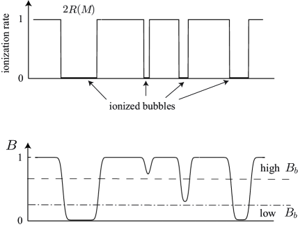
Figure 1: The sketches of ionized bubbles and the smearing effect by the finite observation resolution. Ionized bubbles are fully ionized in the inside of each radius $R(M)$ (top panel). The finite resolution smoothes the signal from ionized bubble. The smoothed surface brightness temperature contrast $B$ for each bubble is different, depending on both the size of ionized bubbles and the resolution size (bottom panel). As a result, each threshold $B_{b}$ gives different number count of ionized bubbles.

As the criterion for the detection of an ionized bubble, we introduce a parameter $B_{b}$. We count bubbles with $B$ smaller than $B_{b}$ as the detectable ones on a 21 cm map (see also Fig. 1). Considering Eqs. (11), (13) and (14), we can relate $B_{b}$ to the limiting mass $M_{\rm lim}$ which is the mass of a collapsed halo associated to an ionized bubble with $B=B_{b}$. Therefore, the number count of ionized bubbles with $B<B_{b}$ is given by

$$N(<B_{b})=\int_{M_{\rm lim}(B_{b})}dM{dV\over dz}{dn\over dM}\Delta z,$$ (15)

where $V$ is a comoving volume and $\Delta z$ is a width of the observation redshift slice. We set $\Delta z=0.1$ throughout this paper.

In Fig. 2, we plot $N(<B_{b})$ as a function of $B_{b}$ for different $f_{NL}$. The 21 cm fluctuations during the epoch of reionization will be mapped by radio interferometric observations. The resolution $\theta_{\rm FWHM}$ for a wave length $\lambda$ depends on its baseline $D$ as $\theta_{\rm FWHM}=\lambda/D$. In the calculation of Fig. 2, we choose two types of the baseline; low resolution type, $D=2~{}$km, which corresponds to the LOFAR baseline, and high resolution type, $D=5~{}$km, which corresponds to the SKA baseline.

As is shown in Fig. 2, the number count strongly depends on the resolution and the redshift of the observation. The large angular resolution smears the ionized bubble whose size is smaller than the resolution. Then, the more the redshift decreases, the larger the number of halos which grow enough to collapse is. In addition, both physical and angular size of a bubble at high redshifts is small compared to the one with the same halo mass at low redshifts. As a result, the number count strongly decreases with increasing of the angular resolution or the redshift. The number count with $B_{b}=0.1$ for the high resolution type at $z=11$ is about 2000, while the number count for the low resolution type at $z=13$ is less than one even for full sky survey with $B_{b}=0.5$ as is shown in Fig. 2.

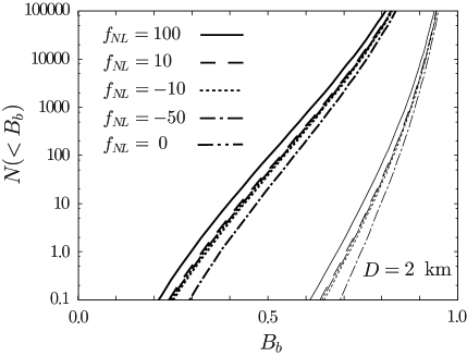
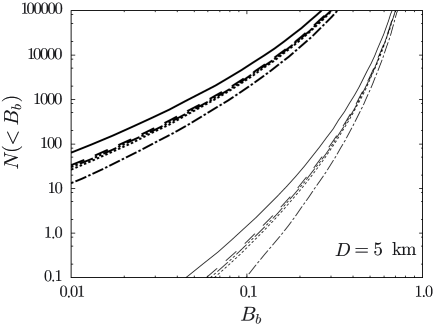
Figure 2: The number count of ionized bubbles as a function of $B_{b}$ for different $f_{NL}$. We plot the number counts for $z=11$ and $z=13$ as the thick and thin lines, respectively. We use the low resolution type ($D=2~{}$km) in the top panel and the high resolution type ($D=5~{}$km) in the bottom.

To make clear the difference of the number counts between the Gaussian and non-Gaussian primordial fluctuations, we plot the ratio of the number counts between non-Gaussian and Gaussian cases as a function of $B_{b}$ in Fig. 3. Producing ionized bubbles during the epoch of reionization is a rare event. Therefore the number counts depend on the degree of the primordial non-Gaussianity. This tendency is emphasized as the redshift increases. The deviation from the Gaussian case becomes larger for all non-Gaussian cases at $z=13$ than at $z=11$. The difference is also enhanced with decreasing $B_{b}$ because lower $B_{b}$ corresponds to higher threshold halo mass $M_{lim}$.

It is shown in Fig. 3 that the dependence on $f_{NL}$ of the number count is more significant for the negative value than the positive one. In the case of negative $f_{NL}$,the high density tail of the distribution function is suppressed, and less number of bubble formation, which is a rare event, takes place. Therefore with decreasing $B_{b}$, the number count rapidly decreases as is shown for $f_{NL}=-50$. On the other hand, for positive $f_{NL}$, the high density tail of the distribution function is enhanced. Accordingly, there are more bubble formation for larger $f_{NL}$. However, the terms proportional to $S_{3}$ and $dS_{3}/dM$ in Eq. (6) have opposite sign in the case of positive $f_{NL}$. Therefore the dependence on $f_{NL}$ is not as strong as in the case of negative $f_{NL}$.

By comparing upper two panels with lower two panels of Fig. 3, we find that deviation from the Gaussian case is larger in the lower resolution observation. However, number counts become smaller for the lower resolution case. As a result, the error of the determination on $f_{NL}$ is expected to be large in the low resolution observation. We discuss this point in the term of signal to noise ratio of the detection later.

In Fig. 4, we show the evolution of the deviation from the Gaussian case with fixing $B_{b}$. In these figures, we adopt the high resolution type and set $B_{b}=0.5$ and $0.1$. The figures tell us that increasing redshift or decreasing $B_{b}$ makes the deviation large. In particular, in high redshift or low $B_{b}$ cases, the number count for the negative $f_{NL}$ case damps rapidly due to the suppression of the bubble formation.

In order to discuss the measurement of $f_{NL}$ by the number count of bubbles, we calculate the Signal to Noise ratio. We assume that the observation instrument is ideal, i.e., there is no instrumental noise, and the foreground noise can be completely removed. Therefore we take into account only the Poisson noise of the number count. The SN ratio for fixed $B_{b}$ is given by

$$S/N=\sqrt{f_{sky}N(<B_{b})},$$ (16)

where $f_{sky}$ is the fraction of sky observed. According to Eq. (16), the large number count gives high SN ratio. Therefore, the larger the threshold $B_{b}$ is set, the higher the SN ratio becomes.

However, setting high threshold makes two problems arise. The first problem is difficulty counting bubbles. In the large $B_{b}$ case, we need to count not only large bubbles but also small bubbles which are hardly seen in a 21 cm map. The second problem is that the deviation from the Gaussian case becomes smaller as $B_{b}$ increases as is shown in Fig. 3. It should be notice that larger S/N does not necessarily mean sensitive to the non-Gaussianity detection. Therefore we need to optimize for the threshold value $B_{b}$ corresponding to the observational settings.

In Fig. 5, we plot the SN ratio with adopting SKA’s field of view ($\sim 100~{}{\rm deg^{2}}$ for 140 MHz), which corresponds to $f_{sky}=2.42\times 10^{-3}$. The top panel of Fig. 5 is for the low resolution ($D=2$ km) and the bottom one is for the high resolution ($D=5$ km). In order to obtain $S/N>5$ for $f_{NL}=100$ for the low resolution at $z=11$ we must set $B_{b}>0.7$ at least. With $B_{b}\sim 0.7$, according to Fig. 2, the number counts for $f_{NL}=100$ is $\sim 20$ for SKA’s field of view, while the one for $f_{NL}=0$ are $\sim 10$ for SKA’s field of view (it should be reminded that Fig. 2 shows the number counts for the full sky survey, $f_{sky}=1$). On the other hand, in the high resolution, $B_{b}>0.1$ is enough to obtain $S/N\sim 5$ for $f_{NL}=100$. In this case, the number count for $f_{NL}=100$ is $\sim 20$, while the one for $f_{NL}=0$ is $\sim 10$ with $S/N\sim 3$. Therefore we conclude that the number count of ionized bubbles has potential to give the constraint on $f_{NL}$.

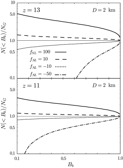
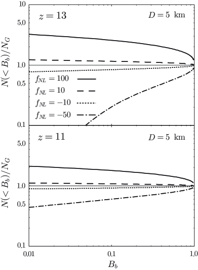
Figure 3: The fractional deviation from the number count for the case of the Gaussian mass function as a function of $B_{b}$. We use the low resolution type ($D=2~{}$km) and the high resolution type ($D=5~{}$km) in the top two panels and the bottom two panels, respectively. In both angular resolution cases, we set $z=13$ and $z=11$. The curves are for $f_{NL}=100$, $f_{NL}=10$, $f_{NL}=-10$ and $f_{NL}=-50$ from top to bottom in both panels.

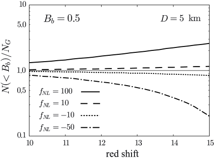
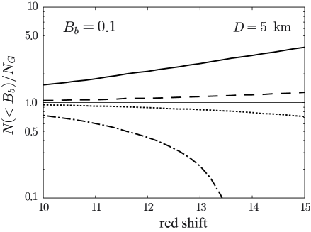
Figure 4: The evolution of the fractional deviation from the number count for the case of the Gaussian mass function as a function of redshift. We set $B_{b}=0.5$ in the top panel and $B_{b}=0.1$ in the bottom panel. The curves are for $f_{NL}=100$, $f_{NL}=10$, $f_{NL}=-10$ and $f_{NL}=-50$ from top to bottom in both panels.

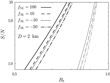
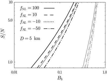
Figure 5: The SN ratio of the number count as a function of $B_{b}$. We set $D=2$ km in the top panel, $D=5$ km in the bottom panel. We assume $f_{sky}=2.42\times 10^{-3}$.

4 conclusion

In this paper, we have studied the number count of ionized bubbles on a 21 cm map as a probe of the primordial non-Gaussianity. Although we have used a simple analytic model of an ionized bubble, such a simple model is enough to illustrate the relation between $f_{NL}$ and the number count of ionized bubbles.

In order to take into account the dependence of the number count on the size of ionized bubbles and the resolution of the observation instrument, we have introduced a threshold parameter $B_{b}$. The bubbles with $B<B_{b}$ are counted as the detectable ionized bubbles on the 21 cm map. Setting smaller $B_{b}$ means counting larger size bubbles. Therefore, we can expect large numbers of ionized bubbles for large $B_{b}$. The deviation of the number count for the non-Gaussian case from the one for the Gaussian case depends on the threshold $B_{b}$. Small $B_{b}$ brings large deviation. However the number count for small $B_{b}$ becomes small. As a result, the SN ratio goes to low. In order to constrain $f_{NL}$ by the number count of ionized bubbles, the optimization between $B_{B}$ and the resolution of observations is needed. For example, in our model, we have found that the number counts for $f_{NL}=100$ and $f_{NL}=0$ for the high resolution with $B_{b}=0.1$ are about $20$ with $S/N\sim 5$ and about $10$ with $S/N\sim 3$, respectively.

The number count also depends on the redshift of a 21 cm map. Compared with the number counts at low redshifts, the ones at high redshifts are lower sensitive to $f_{NL}$. However the number counts at high redshifts are relatively smaller than at low redshifts.Therefore, the SN ratio at high redshifts becomes large and it becomes difficult to give the constraint on $f_{NL}$. Besides, the detection of ionized bubble itself is a challenge (Datta et al., 2007, 2009).

In this paper, we have not taken into account the effect of overlapping of ionized bubbles. The overlaps take place as the universe evolves. As is shown in many reionization simulation works, once overlapping proceeds, the number count of ionized bubbles quickly decreases and the size of ionized bubbles becomes rapidly increasing. Moreover the evolution of the overlapping process depends strongly on the model of reionization. Therefore, our results in this paper can be only adapted for the early phase of the epoch of reionization before the overlapping process takes place.

In order to properly treat the IGM ionization process including overlapping of bubbles, a detailed numerical simulation with radiative transfer is needed. In the near future, we intend to perform the numerical simulation, considering the reionization process.

References

- Bardeen et al. (1983) Bardeen J. M., Steinhardt P. J., Turner M. S., 1983, Phys.Rev.D, 28, 679
- Bartolo et al. (2004) Bartolo N., Komatsu E., Matarrese S., Riotto A., 2004, Phys.Rep, 402, 103
- Battefeld & Easther (2007) Battefeld T., Easther R., 2007, JCAP, 3, 20
- Bromm et al. (2001) Bromm V., Kudritzki R. P., Loeb A., 2001, ApJ, 552, 464
- Chen et al. (2003) Chen X., Cooray A., Yoshida N., Sugiyama N., 2003, MNRAS, 346, L31
- Ciardi & Madau (2003) Ciardi B., Madau P., 2003, ApJ, 596, 1
- Crociani et al. (2009) Crociani D., Moscardini L., Viel M., Matarrese S., 2009, MNRAS, 394, 133
- Curto et al. (2009) Curto A., Martínez-González E., Barreiro R. B., 2009, ApJ, 706, 399
- Datta et al. (2007) Datta K. K., Bharadwaj S., Choudhury T. R., 2007, MNRAS, 382, 809
- Datta et al. (2009) Datta K. K., Bharadwaj S., Choudhury T. R., 2009, MNRAS, 399, L132
- Desjacques & Seljak (2010) Desjacques V., Seljak U., 2010, Classical and Quantum Gravity, 27, 124011
- Falk et al. (1993) Falk T., Rangarajan R., Srednicki M., 1993, ApJL, 403, L1
- Furlanetto et al. (2004) Furlanetto S. R., Zaldarriaga M., Hernquist L., 2004, ApJ, 613, 1
- Gangui et al. (1994) Gangui A., Lucchin F., Matarrese S., Mollerach S., 1994, ApJ, 430, 447
- Grossi et al. (2008) Grossi M., Branchini E., Dolag K., Matarrese S., Moscardini L., 2008, MNRAS, 390, 438
- Guth & Pi (1982) Guth A. H., Pi S., 1982, Physical Review Letters, 49, 1110
- Kamionkowski et al. (2009) Kamionkowski M., Verde L., Jimenez R., 2009, JCAP, 1, 10
- Komatsu et al. (2009) Komatsu E., Dunkley J., Nolta M. R., Bennett C. L., Gold B., Hinshaw G., Jarosik N., Larson D., Limon M., Page L., Spergel D. N., Halpern M., Hill R. S., Kogut A., Meyer S. S., Tucker G. S., Weiland J. L., Wollack E., Wright E. L., 2009, ApJS, 180, 330
- Komatsu & Spergel (2001) Komatsu E., Spergel D. N., 2001, Phys.Rev.D, 63, 063002
- Lo Verde et al. (2008) Lo Verde M., Miller A., Shandera S., Verde L., 2008, Journal of Cosmology and Astro-Particle Physics, 4, 14
- Loeb et al. (2005) Loeb A., Barkana R., Hernquist L., 2005, ApJ, 620, 553
- Madau et al. (1997) Madau P., Meiksin A., Rees M. J., 1997, ApJ, 475, 429
- Matarrese et al. (2000) Matarrese S., Verde L., Jimenez R., 2000, ApJ, 541, 10
- Starobinsky (1982) Starobinsky A. A., 1982, Physics Letters B, 117, 175
- Tozzi et al. (2000) Tozzi P., Madau P., Meiksin A., Rees M. J., 2000, ApJ, 528, 597
- Verde et al. (2000) Verde L., Wang L., Heavens A. F., Kamionkowski M., 2000, MNRAS, 313, 141