Fast Linearized Bregman Iteration for Compressive Sensing and Sparse Denoising

Abstract

We propose and analyze an extremely fast, efficient and simple method for solving the problem:

$$\min\{\|u\|_{1}:Au=f,u\in R^{n}\}.$$

This method was first described in [1], with more details in [2] and rigorous theory given in [3] and [4]. The motivation was compressive sensing, which now has a vast and exciting history, which seems to have started with Candes, et.al. [5] and Donoho, [6]. See [2], [3] and [4] for a large set of references. Our method introduces an improvement called “kicking” of the very efficient method of [1], [2] and also applies it to the problem of denoising of undersampled signals. The use of Bregman iteration for denoising of images began in [7] and led to improved results for total variation based methods. Here we apply it to denoise signals, especially essentially sparse signals, which might even be undersampled.

1 Introduction

Let $A\in R^{m\times n}$, with $n>m$ and $f\in R^{m}$, be given. The aim of a basis pursuit problem is to find $u\in R^{n}$ by solving the constrained minimization problem:

$$\min_{u\in R^{n}}\{J(u)|Au=f\}$$ (1.1)

where $J(u)$ is a continuous convex function.

For basis pursuit, we take:

$$J(u)=|u|_{1}=\sum_{j=1}^{n}|u_{j}|.$$ (1.2)

We assume that $AA^{T}$ is invertible. Thus $Au=f$ is underdetermined and has at least one solution, $u=A^{T}(AA^{T})^{-1}f$, which minimizes the $\ell_{2}$ norm. We also assume that $J(u)$ is coercive, i.e., whenever $\|u\|\rightarrow\infty,\ J(u)\rightarrow\infty$. This implies that the set of all solutions of (1.1) is nonempty and convex. Finally, when $J(u)$ is strictly or strongly convex, the solution of (1.1) is unique.

Basis pursuit arises from many applications. In particular, there has been a recent burst of research in compressive sensing, which involves solving (1.1), (1.2). This was led by Candes et.al. [5], Donoho, [6], and others, see [2], [3] and [4] for extensive references. Compressive sensing guarantees, under appropriate circumstances, that the solution to (1.1), (1.2) gives the sparsest solution satisfying $Au=f$. The problem then becomes one of solving (1.1), (1.2) fast. Conventional linear programming solvers are not tailored for the large scale dense matrices $A$ and the sparse solutions $u$ that arise here. To overcome this, a linearized Bregman iterative procedure was proposed in [1] and analyzed in [2], [3] and [4]. In [2], true, nonlinear Bregman iteration was also used quite successfully for this problem.

Bregman iteration applied to (1.1), (1.2) involves solving the constrained optimization problem through solving a small number of unconstrained optimization problems:

$$\min_{u}\left\{\mu|u|_{1}+\frac{1}{2}\|Au-f\|_{2}^{2}\right\}$$ (1.3)

for $\mu>0$.

In [2] we used a method called the fast fixed point continuation solver (FPC) [8] which appears to be efficient. Other solvers of (1.3) could be used in this Bregman iterative regularization procedure.

Here we will improve and analyze a linearized Bregman iterative regularization procedure, which, in its original incarnation, [1], [2], involved only a two line code and simple operations and was already extremely fast and accurate.

In addition, we are interested in the denoising properties of Bregman iterative regularization, for signals, not images. The results for images involved the BV norm, which we may discretize for $n\times n$ pixel images as:

$$TV(u)=\sum_{i,j=1}^{n-1}((u_{i+1,j}-u_{ij})^{2}+(u_{i,j+1}-u_{ij})^{2})^{\frac{1}{2}}.$$ (1.4)

We usually regard the success of the ROF TV based model [9]

$$\min_{u}\left\{TV(u)+\frac{\lambda}{2}\|f-u\|^{2}\right\}$$ (1.5)

(we now drop the subscript 2 for the $L_{2}$ norm throughout the paper) as due to the fact that images have edges and in fact are almost piecewise constant (with texture added). Therefore, it is not surprising that sparse signals could be denoised using (1.3). The ROF denoising model was greatly improved in [7] and [10] with the help of Bregman iterative regularization. We will do the same thing here using Bregman iteration with (1.3) to denoise sparse signals, with the added touch of undersampling the noisy signals.

The paper is organized as follows: In section 2 we describe Bregman iterative algorithms, as well as the linearized version. We motivate these methods and describe previously obtained theoretical results. In section 3 we introduce an improvement to the linearized version, call “kicking” which greatly speeds up the method, especially for solutions $u$ with a large dynamic range. In section 4 we present numerical results, including sparse recovery for $u$ having large dynamic range, and the recovery of signals in large amounts of noise. In another work in progress [11] we apply these ideas to denoising very blurry and noisy signals remarkably well including sparse recovery for $u$. By blurry we mean situations where $A$ is perhaps a subsampled discrete convolution matrix whose elements decay to zero with $n$, e.g. random rows of a discrete Gaussian.

2 Bregman and Linearized Bregman Iterative Algorithms

The Bregman distance [12], based on the convex function $J$, between points $u$ and $v$, is defined by

$$D_{J}^{p}(u,v)=J(u)-J(v)-\langle p,u-v\rangle$$ (2.6)

where $p\in\partial J(v)$ is an element in the subgradient of $J$ at the point $v$. In general $D_{J}^{p}(u,v)\not=D_{J}^{p}(v,u)$ and the triangle inequality is not satisfied, so $D_{J}^{p}(u,v)$ is not a distance in the usual sense. However it does measure the closeness between $u$ and $v$ in the sense that $D_{J}^{p}(u,v)\geq 0$ and $D_{J}^{p}(u,v)\geq D_{J}^{p}(w,v)$ for all points $w$ on the line segment connecting $u$ and $v$. Moreover, if $J$ is convex, $D_{J}^{p}(u,v)\geq 0$, if $J$ is strictly convex $D_{J}^{p}(u,v)>0$ for $u\not=v$ and if $J$ is strongly convex, then there exists a constant $a>0$ such that

$$D_{J}^{p}(u,v)\geq a\|u-v\|^{2}.$$

To solve (1.1) Bregman iteration was proposed in [2] . Given $u^{0}=p^{0}=0$, we define:

$$u^{k+1} =\arg\min_{u\in R^{n}}\left\{J(u)-J(u^{k})-\langle u-u^{k},p^{k}\rangle+\frac{1}{2}\|Au-f\|^{2}\right\}$$ (2.7)

$$p^{k+1} =p^{k}-A^{T}(Au^{k+1}-f).$$

This can be written as

$$u^{k+1}=\arg\min_{u\in R^{2}}\left\{D_{J}^{p^{k}}(u,u^{k})+\frac{1}{2}\|Au-f\|^{2}\right\}.$$

It was proven in [2] that if $J(u)\in C^{2}(\Omega)$ and is strictly convex in $\Omega$, then $\|Au^{k}-f\|$ decays exponentially whenever $u^{k}\in\Omega$ for all $k$. Furthermore, when $u^{k}$ converges, its limit is a solution of (1.1). It was also proven in [2] that when $J(u)=|u|_{1}$, i.e. for problem (1.1) and (1.2), or when $J$ is a convex function satisfying some additional conditions, the iteration (2.7) leads to a solution of (1.1) in finitely many steps.

As shown in [2], see also [7], [10], the Bregman iteration (2.7) can be written as:

$$f^{k+1} =f^{k}+f-Au^{k}$$

$$u^{k+1} =\arg\min_{u\in R^{n}}\left\{J(u)+\frac{1}{2}\|Au-f^{k+1}\|^{2}\right\}$$ (2.8)

This was referred to as “adding back the residual” in [7] . Here $f^{0}=0,u^{0}=0$. Thus the Bregman iteration uses solutions of the unconstrained problem

$$\min_{u\in R}\left\{J(u)+\frac{1}{2}\|Au-f\|^{2}\right\}$$ (2.9)

as a solver in which the Bregman iteration applies this process iteratively.

Since there is generally no explicit expression for the solver of (2.7) or (2.8), we turn to iterative methods. The linearized Bregman iteration which we will analyze, improve and use here is generated by

$$u^{k+1} =\arg\min_{u\in R^{n}}\left\{J(u)-J(u^{k})-\langle u-u^{k},p^{k}\rangle+\frac{1}{2\delta}\|u-(u^{k}-\delta A^{T}(Au^{k}-f))\|^{2}\right\}$$

$$p^{k+1} =p^{k}-\frac{1}{\delta}(u^{k+1}-u^{k})-A^{T}(Au^{k}-f).$$ (2.10)

In the special case considered here, where $J(u)=\mu\|u\|_{1}$, then we have the two line algorithm

$$v^{k+1} =v^{k}-A^{T}(Au^{k}-f)$$ (2.11)

$$u^{k+1} =\delta\cdot\text{shrink}(v^{k+1},\mu)$$ (2.12)

where $v^{k}$ is an auxiliary variable

$$v^{k}=p^{k}+\frac{1}{\delta}u^{k}$$ (2.13)

and

$$\text{shrink}(x,\mu):=\begin{cases}x-\mu,&\text{if}\ x>\mu\\ 0,&\text{if}\ -\mu\leq x\leq\mu\\ x+\mu,&\text{if}\ x<-\mu\end{cases}$$

is the soft thresholding algorithm [13] .

This linearized Bregman iterative algorithm was invented in [1] and used and analyzed in [2],[3] and [4]. In fact it comes from the inner-outer iteration for (2.7). In [2] it was shown that the linearized Bregman iteration (2.10) is just one step of the inner iteration for each outer iteration. Here we repeat the arguments also in [2], which begin by summing the second equation in (2.10) arriving at (using the fact that $u^{0}=p^{0}=0$):

$$p^{k}+\dfrac{1}{\delta}u^{k}+\sum_{j=0}^{k-1}A^{T}(Au^{j}-f)=p^{k}+\dfrac{1}{\delta}u^{k}-v^{k}=0,\ \text{for}\ k=1,2,\ldots.$$

This gives us (2.12), and allows us to rewrite its first equation as:

$$u^{k+1}=\arg\min_{u\in R^{n}}\left\{J(u)+\frac{1}{2\delta}\|u-\delta v^{k+1}\|^{2}\right\}$$ (2.14)

i.e. we are adding back the “linearized noise”, where $v^{k+1}$ is defined in (2.11).

In [2] and [3] some interesting analysis was done for (2.10), (and some for (2.14)). This was done first for $J(u)$ continuously differentiable in (2.10) and the gradient $\partial J(u)$ satisfying

$$\|\partial J(u)-\partial J(v)\|^{2}\leq\beta\langle\partial J(u)-\partial J(v),u-v\rangle,$$ (2.15)

$\forall u,v\in R^{n},\ \beta>0$. In [3] it was shown that, if (2.15) is true, then both of the sequences $(u^{k})_{k\in N}$ and $(p^{k})_{k\in N}$ defined by (2.10) converge for $0<\delta<\frac{2}{\|AA^{T}\|}$.

In [4] the authors recently give a theoretical analysis, showing that the iteration in (2.11) and (2.12) converges to the unique solution of

$$\min_{u\in R^{n}}\left\{\mu\|u\|_{1}+\frac{1}{2\delta}\|u\|^{2}:Au=f\right\}$$ (2.16)

They also show the interesting result: let $S$ be the set of all solutions of the Basis Pursuit problem (1.1), (1.2) and let

$$u_{1}=\arg\min_{u\in S}\|u\|^{2}$$ (2.17)

which is unique. Denote the solution of (2.16) as $u_{\mu}^{*}$. Then

$$\lim_{\mu\rightarrow\infty}\|u_{\mu}^{*}-u_{1}\|=0.$$ (2.18)

In passing they show that

$$\|u_{\mu}^{*}\|\leq\|u_{1}\|\ \text{for all}\ \mu>0$$ (2.19)

which we will use below.

Another theoretical analysis on Linearized Bregman algorithm is given by Yin in [14], where he shows that Linearized Bregman iteration is equivalent to gradient descent applied to the dual of the problem (2.16) and uses this fact to obtain an elegant convergence proof.

This summarizes the relevant convergence analysis for our Bregman and linearized Bregman models.

Next we recall some results from [7] regarding noise and Bregman iteration.

For any sequence $\{u^{k}\},\{p^{k}\}$ satisfying (2.7) for $J$ continuous and convex, we have, for any $\tilde{\mu}$

$$D_{J}^{p^{k}}(\tilde{u},u^{k})-D_{J}p^{k-1}(\tilde{u},u^{k-1})\leq\langle A\tilde{u}-f,Au^{k-1}-f\rangle-\|Au^{k-1}-f\|^{2}.$$ (2.20)

Besides implying that the Bregman distance between $u^{k}$ and any element $\tilde{u}$ satisfying $A\tilde{u}=f$ is monotonically decreasing, it also implies that, if $\tilde{u}$ is the “noise free” approximation to the solution of (1.1), the Bregman distance between $u^{k}$ and $\tilde{u}$ diminishes as long as

$$\|Au^{k}-f\|>\|A\tilde{u}-f\|=\sigma,\ \text{where}\ \sigma\ \text{is some measure of the noise}$$ (2.21)

i.e., until we get too close to the noisy signal in the sense of (2.21). Note, in [7] we took $A$ to be the identity, but these more general results are also proven there. This gives us a stopping criterion for our denoising algorithm.

In [7] we obtained a result for linearized Bregman iteration, following [15], which states that the Bregman distance between $\tilde{u}$ and $u^{k}$ diminish as long as

$$\|A\tilde{u}-f\|<(1-2\delta\|AA^{T}\|)\ \|Au^{k}-f\|$$ (2.22)

so we need $0<2\delta\|AA^{T}\|<1$.

In practice, we will use (2.21) as our stopping criterion.

3 Convergence

We begin with the following simple results for the linearized Bregman iteration or the equivalent algorithm (2.10).

Theorem 3.1.

If $u^{k}\rightarrow u^{\infty}$, then $Au^{\infty}=f$.

Proof.

Assume $Au^{\infty}\not=f$. Then $A^{T}(Au^{\infty}-f)\not=0$ since $A^{T}$ has full rank. This means that for some $i$, $(A^{T}(Au^{k}-f))_{i}$ converges to a nonzero value, which means that $v_{i}^{k+1}-v_{i}^{k}$ does as well. On the other hand $\{v^{k}\}=\{u^{k}/\delta+p^{k}\}$ is bounded since $\{u^{k}\}$ converges and $p^{k}\in[-\mu,\mu]$. Therefore $\{v_{i}^{k}\}$ is bounded, while $v_{i}^{k+1}-v_{i}^{k}$ converges to a nonzero limit, which is impossible. ∎

Theorem 3.2.

If $u^{k}\rightarrow u^{\infty}$ and $v^{k}\rightarrow v^{\infty}$, then $u^{\infty}$ minimizes $\{J(u)+\frac{1}{2\delta}\|u\|^{2}:Au=f\}$.

Proof.

Let $\tilde{J}(u)=J(u)+\frac{1}{2\delta}\|u\|^{2}$. then

$$\partial\tilde{J}(u)=\partial J(u)+\frac{1}{\delta}u.$$

Since $\partial J(u^{k})=p^{k}=v^{k}-u^{k}/\delta$, we have $\partial\tilde{J}(u^{k})=v^{k}$. Using the non-negativity of the Bregman distance we obtain

$$\tilde{J}(u^{k}) \leq\tilde{J}(u_{\text{opt}})-\langle u_{\text{opt}}-u^{k},\partial\tilde{J}(u^{k})\rangle$$

$$=\tilde{J}(u_{\text{opt}})-\langle u_{\text{opt}}-u^{k},v^{k}\rangle$$

where $u_{\text{opt}}$ minimizes (1.1) with $J$ replaced by $\tilde{J}$, which is strictly convex.

Let $k\rightarrow\infty$, we have

$$\tilde{J}(u^{\infty})\leq\tilde{J}(u_{\text{opt}})-\langle u_{\text{opt}}-u^{\infty},v^{\infty}\rangle$$

Since $v^{k}=A^{T}\sum_{j=0}^{k-1}A^{T}(f-Au^{j})$, we have $v^{\infty}\in\text{range}(A^{T})$. Since $Au_{\text{opt}}=Au^{\infty}=f$, we have $\langle u_{\text{opt}}-u^{\infty},v^{\infty}\rangle=0$, which implies $\tilde{J}(u^{\infty})\leq\tilde{J}(u_{\text{opt}})$. ∎

Equation (2.16) (from a result in [3] ) implies that $u^{\infty}$ will approach a solution to (1.1), (1.2), as $\mu$ approaches $\infty$.

The linearized Bregman iteration has the following monotonicity property:

Theorem 3.3.

If $u^{k+1}\not=u^{k}$ and $0<\delta<2/\|AA^{T}\|$, then

$$\|Au^{k+1}-f\|<\|Au^{k}-f\|.$$

Proof.

Let

$$u^{k+1}-u^{k}=\Delta u^{k},\ v^{k+1}-v^{k}=\Delta v^{k}.$$

Then the shrinkage operation is such that

$$\Delta u_{i}^{k}=\delta q_{i}^{k}\Delta v_{i}^{k}$$ (3.23)

with

$$q_{i}^{k}\begin{cases}=1&\text{if}\ u_{i}^{k+1}u_{i}^{k}>0\\ =0&\text{if}\ u_{i}^{k+1}=u_{i}^{k}=0\\ \in(0,1]&\text{otherwise}\end{cases}$$

Let $Q^{k}=\text{Diag}~{}(q_{i}^{k})$. Then (3.23) can be written as

$$\Delta u^{k}=\delta Q^{k}\Delta v^{k}=\delta Q^{k}A^{T}(f-Au^{k})$$ (3.24)

which implies

$$Au^{k+1}-f=(I-\delta AQ^{k}A^{T})(Au^{k}-f).$$ (3.25)

From (3.23), $Q^{k}$ is diagonal with $0\preceq Q^{k}\preceq I$, so $0\preceq AQ^{k}A^{T}\preceq AA^{T}$. If we choose $\delta>0$ such that $\delta AA^{T}\prec 2I$, then $0\preceq\delta AQ^{k}A^{T}\prec 2I$ or $-I\prec I-\delta AQ^{k}A^{T}\preceq I$ which implies that $\|Au^{k}-f\|$ is not increasing. To get strict decay, we need only show that $AQ^{k}A^{T}(Au^{k}-f)=0$ is impossible if $u^{k+1}\not=u^{k}$. Suppose $AQ^{k}A^{T}(Au^{k}-f)=0$ holds, then from (3.24) we have:

$$\langle\Delta u^{k},\Delta v^{k}\rangle=\delta\langle A^{T}(f-Au^{k}),Q^{k}A^{T}(f-Au^{k})\rangle=0.$$

By (3.23), this only happens if $u_{i}^{k+1}=u_{i}^{k}$ for all $i$, which is a contradiction. ∎

We are still faced with estimating how fast the residual decays. It turns out that if consecutive elements of $u$ do not change sign, then $\|Au-f\|$ decays exponentially. By ’exponential’ we mean that the ratio of the residuals of two consecutive iteration converges to a constant, this type of convergence is sometimes called linear convergence. Here we define

$$S_{u}=\{x\in R^{n}:\text{sign}(x_{i})=\text{sign}(u_{i}),\forall i\}$$ (3.26)

(where $\text{sign}(0)=0$ and $\text{sign}(a)=a/|a|$ for $a\neq 0$). Then we have the following:

Theorem 3.4.

If $u^{k}\in S\equiv S_{u_{k}}$ for $k\in(T_{1},T_{2})$, then $u^{k}$ converges to $u^{*}$, where $u^{*}\in\arg\min\{\|Au-f\|^{2}:u\in S\}$ and $\|Au^{k}-f\|^{2}$ decays to $\|Au^{*}-f\|^{2}$ exponentially.

Proof.

. Since $u^{k}\in S$ for $k\in[T_{1},T_{2}]$, we can define $Q\equiv Q^{k}$ for $T_{1}\leq k\leq T_{2}-1$. From (3.23) we see that $Q^{k}$ is a diagonal matrix consisting of zeros or ones, so $Q=Q^{T}Q$. Moreover, it is easy to see that $S=\{x|Qx=x\}$.

Following the argument in Theorem 3.3 we have:

$$u^{k+1}-u^{k}=\Delta u^{k}=\delta Q\Delta v^{k}=\delta QA^{T}(f-Au^{k})$$ (3.27)

$$Au^{k+1}-f=[I-\delta AQA^{T}](Au^{k}-f)$$ (3.28)

and

$$-I\prec I-\delta AQA^{T}\preceq I.$$

Let $R^{n}=V_{0}\oplus V_{1}$, where $V_{0}$ is the null space of $AQA^{T}$ and $V_{1}$ is spanned by the eigenvectors corresponding to the nonzero eigenvalues of $AQA^{T}$. Let $Au^{k}-f=w^{k,0}+w^{k,1}$, where $w^{k,j}\in V_{j}$ for $j=0,1$. From (3.28) we have

$$w^{k+1,0} = w^{k,0}$$

$$w^{k+1,1} = [I-\delta AQA^{T}]w^{k,1}$$

for $T_{1}\leq k\leq T_{2}-1$. Since $w^{k,1}$ is not in the null space of $AQA^{T}$, then (3.27) and (3.28) imply that $\|w^{k,1}\|$ decays exponentially. Let $w^{0}=w^{k,0}$, then $AQA^{T}w^{0}=0$ $AQQA^{T}w^{0}\Rightarrow QA^{T}w^{0}=0$. Therefore, from (3.27) we have

$$\Delta u^{k}=\delta Q^{T}A^{T}(f-Au^{k})=\delta QA^{T}(w^{0}+w^{k,1})=\delta QA^{T}w^{k,1}.$$

Thus $\|\Delta u^{k}\|$ decays exponentially. This means $\{u^{k}\}$ forms a Cauchy sequence in $S$, so it has a limit $u^{*}\in S$. Moreover

$$Au^{*}-f=\lim_{k}(Au^{k}-f)=\lim_{k}w^{k,0}+\lim_{k}w^{k,1}=w^{0}.$$

Since $V_{0}$ and $V_{1}$ are orthogonal:

$$\|Au^{k}-f\|^{2}=\|w^{k,0}\|^{2}+\|w^{k,1}\|^{2}=\|Au^{*}-f\|^{2}+\|w^{k,1}\|^{2},$$

so $\|Au^{k}-f\|^{2}-\|Au^{*}-f\|^{2}$ decays exponentially. The only thing left to show is that

$$u^{*}=\arg\min(\|Au-f\|^{2}:u\in S)=\arg\min\{\|Au-f\|^{2}:Qu=u\}.$$

This is equivalent to way that $A^{T}(Au^{*}-f)$ is orthogonal with the hyperspace $\{u:Qu=u\}$. It’s easy to see that since $Q$ is a projection operator, a vector $v$ is orthogonal with $\{u:Qu=u\}$ if and only if $Qv=0$, thus we need to show $QA^{T}(Au^{*}-f)=0$. This is obvious because we have shown that $Au^{*}-f=w^{0}$ and $QA^{T}w^{0}=0$. So we find that $u^{*}$ is the desired minimizer. ∎

Therefore, instead of decaying exponentially with a global rate, the residual of the linearized Bregman iteration decays in a rather sophisticated manner. From the definition of the shrinkage function we can see that the sign of an element of $u$ will change if and only if the corresponding element of $v$ crosses the boundary of the interval $[-\mu,\mu]$. If $\mu$ is relatively large compared with the size of $\Delta v$ (which is usually the case when applying the algorithm to a compressed sensing problem), then at most iterations the signs of the elements of $u$ will stay unchanged, i.e. $u$ will stay in the subspace $S_{u}$ defined in (3.26) for a long while. This theorem tells us that under this scenario $u$ will quickly converge to the point $u^{*}$ that minimizes $\|Au-f\|$ inside $S_{u}$, and the difference between $\|Au-f\|$ and $\|Au^{*}-f\|$ decays exponentially. After $u$ converges to $u^{*}$, $u$ will stay there until the sign of some element of $u$ changes. Usually this means that a new nonzero element of $u$ comes up. After that, $u$ will enter a different subspace $S$ and a new converging procedure begins.

The phenomenon described above can be observed clearly in Fig 1. The final solution of $u$ contains five non-zero spikes. Each time a new spike appears, it converges rapidly to the position that minimizes $\|Au-f\|$ in the subspace $S_{u}$. After that there is a long stagnation, which means $u$ is just waiting there until the accumulating $v$ brings out a new non-zero element of $u$. The larger $\mu$ is, the longer the stagnation takes. Although the convergence of the residual during each phase is fast, the total speed of the convergence suffers much from the stagnation. The solution of this problem will be described in the next section.

Figure 1: The left figure presents a simple signal with 5 non-zero spikes. The right figure shows how the linearized Bregman iteration converges.

4 Fast Implementation

The iterative formula in Algorithm 1 below gives us the basic linearized Bregman algorithm designed to solve (1.1),(1.2).

Algorithm 1 Bregman Iterative Regularization

  Initialize: $u=0$, $v=0$.

  while “$\|f-Au\|$ not converge” do

     $v^{k+1}=v^{k}+A^{\top}(f-Au^{k})$

     $u^{k+1}=\delta\cdot\text{shrink}(v^{k+1},\mu)$

  end while

This is an extremely concise algorithm, simple to program, involve only matrix multiplication and shrinkage. When $A$ consists of rows of a matrix of a fast transform like FFT which is a common case for compressed sensing, it is even faster because matrix multiplication can be implemented efficiently using the existing fast code of the transform. Also, storage becomes a less serious issue.

We now consider how we can accelerate the algorithm under the problem of stagnation described in the previous section. From that discussion, during a stagnation $u$ converges to a limit $u^{*}$ so we will have $u^{k+1}\approx u^{k+2}\approx\cdots\approx u^{k+m}\approx u^{*}$ for some $m$. Therefore the increment of $v$ in each step, $A^{\top}(f-Au)$, is fixed. This implies that during the stagnation $u$ and $v$ can be calculated explicitly as following

$$\begin{cases}u^{k+j}\equiv u^{k+1}\\ v^{k+j}=v^{k}+j\cdot A^{\top}(f-Au^{k+1})\end{cases}j=1,\cdots,m$$ (4.29)

If we denote the set of indices of the zero elements of $u^{*}$ as $I_{0}$ and let $I_{1}=\overline{I_{0}}$ be the support of $u^{*}$, then $v^{k}_{i}$ will keep changing only for $i\in I_{0}$ and the iteration can be formulated entry-wise as:

$$\begin{cases}u^{k+j}_{i}\equiv u^{k+1}_{i}&\forall i\\ v^{k+j}_{i}=v^{k}_{i}+j\cdot(A^{\top}(f-Au^{k+1}))_{i}&i\in I_{0}\\ v^{k+j}_{i}\equiv v^{k+1}_{i}&i\in I_{1}\end{cases}$$ (4.30)

for $j=1,\cdots,m$. The stagnation will end when $u$ begins to change again. This happens if and only if some element of $v$ in $I_{0}$ (which keeps changing during the stagnation) crosses the boundary of the interval $[-\mu,\mu]$. When $i\in I_{0}$, $v^{k}_{i}\in[-\mu,\mu]$, so we can estimate the number of the steps needed for $v_{i}^{k}$ to cross the boundary $\forall i\in I_{0}$ from (4.30), which is

$$s_{i}=\left\lceil\dfrac{\mu\cdot\text{sign}((A^{\top}(f-Au^{k+1}))_{i})-v^{k+1}_{i}}{(A^{\top}(f-Au^{k+1}))_{i}}\right\rceil\,\forall i\in I_{0}$$ (4.31)

and

$$s=\min_{i\in I_{0}}\{s_{i}\}$$ (4.32)

is the number of steps needed. Therefore, $s$ is nothing but the length of the stagnation. Using (4.29), we can predict the end status of the stagnation by

$$\begin{cases}u^{k+s}\equiv u^{k+1}\\ v^{k+s}=v^{k}+s\cdot A^{\top}(f-Au^{k+1})\end{cases}j=1,\cdots,m$$ (4.33)

Therefore, we can kick $u$ to the critical point of the stagnation when we detect that $u$ has been staying unchanged for a while. Specifically, we have the following algorithm: Algorithm 2.

Algorithm 2 Linearized Bregman Iteration with Kicking

  Initialize: $u=0$, $v=0$.

  while “$\|f-Au\|$ not converge” do

     if “$u^{k-1}\approx u^{k}$” then

        calculate $s$ from (4.31) and (4.32)

        $v^{k+1}_{i}=v^{k}_{i}+s\cdot(A^{\top}(f-Au^{k}))_{i}$, $\forall i\in I_{0}$

        $v^{k+1}_{i}=v^{k}_{i}$, $\forall i\in I_{1}$

     else

        $v^{k+1}=v^{k}+A^{\top}(f-Au^{k})$

     end if

     $u^{k+1}=\delta\cdot\text{shrink}(v^{k+1},\mu)$

  end while

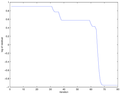
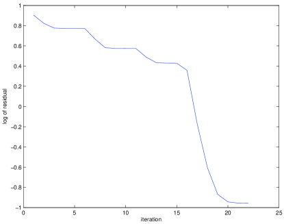
Figure 2: The left figure presents the convergence curve of the original linearized Bregman iteration using the same signal as Fig 1. The right figure shows the convergence curve of the linearized Bregman iteration with the kicking modification.

Indeed, this kicking procedure is similar to line search commonly used in optimization problems and modifies the initial algorithm in no way but just accelerates the speed. More precisely, note that the output sequence $\{u^{k},v^{k}\}$ is a subsequence of the original one, so all the previous theoretical conclusions on convergence still hold here.

An example of the algorithm is shown in Fig 2. It is clear that all the stagnation in the original convergence collapses to single steps. The total amount of computation is reduced dramatically.

5 Numerical Results

In this section, we demonstrate the effectiveness of the algorithm (with kicking) in solving basis pursuit and some related problems.

5.1 Efficiency

Consider the constrained minimization problem

$$\min|u|_{1}\quad\mbox{s.t. }Au=f,$$

where the constraints $Au=f$ are under-determined linear equations with $A$ an $m\times n$ matrix, and $f$ generated from a sparse signal $\bar{u}$ that has a number of nonzeros $\kappa<m$.

Our numerical experiments use two types of $A$ matrices: Gaussian matrices whose elements were generated from i.i.d. normal distributions $\mathcal{N}(0,1)$ (randn(m,n) in MATLAB), and partial discrete cosine transform (DCT) matrices whose $k$ rows were chosen randomly from the $n\times n$ DCT matrix. These matrices are known to be efficient for compressed sensing. The number of rows $m$ is chosen as $m\sim\kappa\log(n/\kappa)$ for Gaussian matrices and $m\sim\kappa\log n$ for DCT matrices (following [5] ).

The tested original sparse signals $\bar{u}$ had numbers of nonzeros equal to $0.05n$ and $0.02n$ rounded to the nearest integers in two sets of experiments, which were obtained by round(0.05*n) and round(0.02*n) in MATLAB, respectively. Given a sparsity $\|\bar{u}\|_{0}$, i.e., the number of nonzeros, an original sparse signal $\bar{u}\in\mathbb{R}^{n}$ was generated by randomly selecting the locations of $\|\bar{u}\|_{0}$ nonzeros, and sampling each of these nonzero elements from $\mathcal{U}(-1,1)$ (2*(rand-0.5) in MATLAB). Then, $f$ was computed as $A\bar{u}$. When $\|\bar{u}\|_{0}$ is small enough, we expect the basis pursuit problem, which we solved using our fast algorithm, to yield a solution $u^{*}=\bar{u}$ from the inputs $A$ and $f$.

Note that partial DCT matrices are implicitly stored fast transforms for which matrix-vector multiplications in the forms of $Ax$ and $A^{\top}x$ were computed by the MATLAB commands dct(x) and idct(x), respectively. Therefore, we were able to test on partial DCT matrices of much larger sizes than Gaussian matrices. The sizes $m$-by-$n$ of these matrices are given in the first two columns of Table 1.

Our code was written in MATLAB and was run on a Windows PC with a Intel(R) Core(TM) 2 Duo 2.0GHz CPU and 2GB memory. The MATLAB version is 7.4.

The set of computational results given in Table 1 was obtained by using the stopping criterion

$$\frac{\|Au^{k}-f\|}{\|f\|}<10^{-5},$$ (5.34)

which was sufficient to give a small error $\|u^{k}-\bar{u}\|/\|\bar{u}\|$. Throughout our experiments in Table 1, we used $\mu=1$ to ensure the correctness of the results.

Table 1: Experiment results using 10 random instances for each configuration of $(m,n,\|\bar{u}\|_{0})$, with nonzero elements of $\bar{u}$ come from $\mathcal{U}(-1,1)$.

Results of linearized Bregman-$L_{1}$ with kicking
Stopping tolerance.			$\|Au^{k}-f\|/\|f\|<10^{-5}$
		Gaussian matrices
		stopping itr. $k$			relative error $\|u^{k}-\bar{u}\|/\|\bar{u}\|$			time (sec.)
		mean	std.	max	mean	std.	max	mean	std.	max
$n$	$m$	$\|\bar{u}\|_{0}=0.05n$
1000	300	422	67	546	2.0e-05	4.3e-06	2.7e-05	0.42	0.06	0.51
2000	600	525	57	612	1.8e-05	1.9e-06	2.1e-05	4.02	0.45	4.72
4000	1200	847	91	1058	1.7e-05	1.7e-06	1.9e-05	25.7	2.87	32.1
$n$	$m$	$\|\bar{u}\|_{0}=0.02n$
1000	156	452	98	607	2.3e-05	2.6e-06	2.6e-05	0.24	0.06	0.33
2000	312	377	91	602	2.0e-05	4.0e-06	2.9e-05	1.45	0.38	2.37
4000	468	426	30	477	1.6e-05	2.1e-06	2.0e-05	6.96	0.51	7.94
		Partial DCT matrices
$n$	$m$	$\|\bar{u}\|_{0}=0.05n$
4000	2000	71	6.6	82	9.1e-06	2.5e-06	1.2e-05	0.43	0.06	0.56
20000	10000	158	14.5	186	6.2e-06	2.1e-06	1.1e-05	3.95	0.36	4.73
50000	25000	276	14	296	6.8e-06	2.6e-06	1.0e-05	17.6	0.99	19.2
$n$	$m$	$\|\bar{u}\|_{0}=0.02n$
4000	1327	52	7.0	64	8.6e-06	1.3e-06	1.1e-05	0.27	0.04	0.35
20000	7923	91	10.3	115	7.2e-06	2.2e-06	1.1e-05	2.36	0.30	3.02
50000	21640	140	9.7	153	5.9e-06	2.4e-06	1.1e-05	8.53	0.66	9.42

5.2 Robustness to Noise

In real applications, the measurement $f$ we obtain is usually contaminated by noise. The measurement we have is:

$$\tilde{f}=f+n=A\bar{u}+n,\quad n\in\mathcal{N}(0,\sigma).$$

To characterize the noise level, we shall use SNR (signal to noise ratio) instead of $\sigma$ itself. The SNR is defined as follows

$$SNR(u):=20\log_{10}(\frac{\|\bar{u}\|}{\|n\|}).$$

In this section we test our algorithm on recovering the true signal $\bar{u}$ from $A$ and the noisy measurement $\tilde{f}$. As in the last section, the nonzero entries of $\bar{u}$ are generated from $\mathcal{U}(-1,1)$, and $A$ is either a Gaussian random matrix or a partial DCT matrix. Our stopping criteria is given by

$$\mbox{std}\big{(}Au^{k}-\tilde{f}\big{)}<\sigma,\quad\mbox{and}\quad\mbox{Iter.}<1000,$$

i.e. we stop whenever the standard deviation of residual $Au^{k}-\tilde{f}$ is less than $\sigma$ or the number of iterations exceeds $1000$. Table 2 shows numerical results for different noise level, size of $A$ and sparsity. We also show one typical result for a partial DCT matrix with size $n=4000$ and $\|\bar{u}\|_{0}=0.02n=80$ in Figure 3.

Table 2: Experiment results using 10 random instances for each configuration of $(m,n,\|\bar{u}\|_{0})$.

Results of linearized Bregman-$L_{1}$ with kicking
Stopping criteria.			$\mbox{std}(Au^{k}-f)<\sigma$.
		Gaussian matrices
		stopping itr. $k$			relative error $\|u^{k}-\bar{u}\|/\|\bar{u}\|$			time (sec.)
		mean	std.	max	mean	std.	max	mean	std.	max
Avg. SNR	($n$,$m$)	$\|\bar{u}\|_{0}=0.05n$
26.12	(1000,300)	420	95	604	0.0608	0.0138	0.0912	0.33	0.09	0.53
25.44	(2000,600)	206	32	253	0.0636	0.0128	0.0896	1.49	0.22	1.79
26.02	(4000,1200)	114	11	132	0.0622	0.0079	0.0738	3.32	0.31	3.81
Avg. SNR	($n$,$m$)	$\|\bar{u}\|_{0}=0.02n$
27.48	(1000,156)	890	369	1612	0.0456	0.0085	0.0599	0.42	0.17	0.73
25.06	(2000,312)	404	64	510	0.0638	0.0133	0.0843	1.37	0.23	1.74
26.04	(4000,468)	216	35	267	0.0557	0.0068	0.0639	3.29	0.55	4.13
		Partial DCT matrices
Avg. SNR	($n$,$m$)	$\|\bar{u}\|_{0}=0.05n$
23.97	(4000, 2000)	151	9.2	170	0.0300	0.0028	0.0332	0.94	0.07	1.03
24.00	(20000,10000)	250	14	270	0.0300	0.0010	0.0318	7.88	0.62	8.86
24.09	(50000,25000)	274	9.9	295	0.0304	0.0082	0.0315	20.4	0.74	20.1
Avg. SNR	($n$,$m$)	$\|\bar{u}\|_{0}=0.02n$
24.29	(4000,1327)	130	11	157	0.0223	0.0023	0.0253	0.79	0.08	1.00
24.37	(20000,7923)	223	14	257	0.0204	0.0025	0.0242	6.89	0.53	8.15
24.16	(50000,21640)	283	19	311	0.0193	0.0012	0.0207	21.5	1.68	24.1

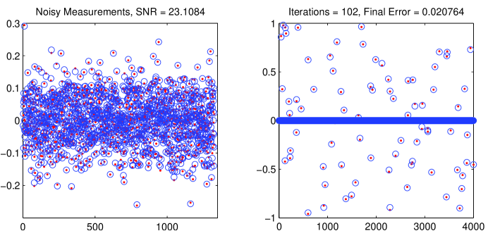
Figure 3: The left figure presents the clean (red dots) and noisy (blue circles) measurements, with SNR=23.1084; the right figure shows the reconstructed signal (blue circles) v.s. original signal (red dots), where the relative error=0.020764, and number of iterations is 102.

5.3 Recovery of Signal with High Dynamical Range

In this section, we test our algorithm on signals with high dynamical ranges. Precisely speaking, let $\mbox{MAX}=\max\{|\bar{u}_{i}|:i=1,\ldots,n\}$ and $\mbox{MIN}=\min\{|u_{i}|:u_{i}\neq 0,i=1,\ldots,n\}$. The signals we shall consider here satisfy $\frac{\mbox{MAX}}{\mbox{MIN}}\approx 10^{10}$. Our $\bar{u}$ is generated by multiplying a random number in $[0,1]$ with another one randomly picked from $\{1,10,\ldots,10^{10}\}$. Here we adopt the stopping criteria

$$\frac{\|Au^{k}-f\|}{\|f\|}<10^{-11}$$

for the case without noise (Figure 4) and the same stopping criteria as in the previous section for the noisy cases (Figures 5-7). In the experiments, we take the dimension $n=4000$, the number of nonzeros of $\bar{u}$ to be $0.02n$, and $\mu=10^{10}$. Here $\mu$ is chosen to be much larger than before, because the dynamical range of $\bar{u}$ is large. Figure 4 shows results for the noise free case, where the algorithm converges to a $10^{-11}$ residual in less than 300 iterations. Figures 5-7 show the cases with noise (the noise is added the same way as in previous section). As one can see, if the measurements are contaminated with less noise, signals with smaller magnitudes will be recovered well. For example in Figure 5, the SNR$\approx 118$, and the entries of magnitudes $10^{4}$ are well recovered; in Figure 6, the SNR$\approx 97$, and the entries of magnitudes $10^{5}$ are well recovered; and in Figure 7, the SNR$\approx 49$, and the entries of magnitudes $10^{7}$ are well recovered.

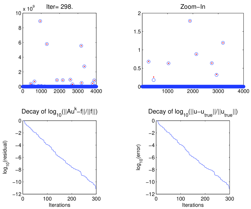
Figure 4: Upper left, true signal (red dots) v.s. recovered signal (blue circle); upper right, one zoom-in to the lower magnitudes; lower left, decay of residual $\log_{10}\frac{\|Au^{k}-f\|}{\|f\|}$; lower right, decay of error to true solution $\log_{10}\frac{\|u^{k}-\bar{u}\|}{\|\bar{u}\|}$.

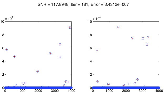
Figure 5: Noisy case. Left figure, true signal (red dots) v.s. recovered signal (blue circle); right figure, one zoom-in to the magnitude$\approx 10^{5}$. The error is measured by $\frac{\|u^{k}-\bar{u}\|}{\|\bar{u}\|}$.

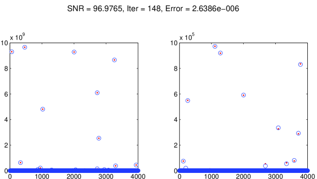
Figure 6: Noisy case. Left figure, true signal (red dots) v.s. recovered signal (blue circle); right figure, one zoom-in to the magnitude$\approx 10^{6}$. The error is measured by $\frac{\|u^{k}-\bar{u}\|}{\|\bar{u}\|}$.

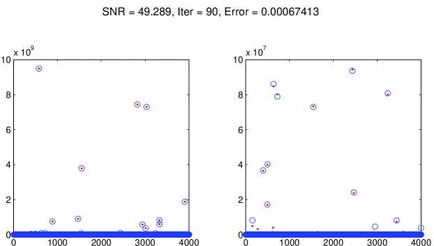
Figure 7: Noisy case. Left figure, true signal (red dots) v.s. recovered signal (blue circle); right figure, one zoom-in to the magnitude$\approx 10^{8}$. The error is measured by $\frac{\|u^{k}-\bar{u}\|}{\|\bar{u}\|}$.

5.4 Recovery of Sinusoidal Waves in Huge Noise

In this section we consider

$$\bar{u}(t)=a\sin(\alpha t)+b\cos(\beta t),$$

where $a,b,\alpha$ and $\beta$ are unknown. The observed signal $\tilde{u}$ is noisy and has the form $\tilde{u}=\bar{u}+n$ with $n\sim\mathcal{N}(0,\sigma)$. In practice, the noise in $\tilde{u}$ could be huge, i.e. possibly have a negative SNR, and we may only be able to observe partial information of $\tilde{u}$, i.e. only a subset of values of $\tilde{u}$ is known. Notice that the signal is sparse (only four spikes) in frequency domain. Therefore, this is essentially a compressed sensing problem and $\ell_{1}$-minimization should work well here. Now the problem can be stated as reconstructing the original signal $\bar{u}$ from random samples of the observed signal $\tilde{u}$ using our fast $\ell_{1}$-minimization algorithm. In our experiments, the magnitudes $a$ and $b$ are generated from $\mathcal{U}(-1,1)$; frequencies $\alpha$ and $\beta$ are random multiples of $\frac{2\pi}{n}$, i.e. $\alpha=k_{1}\frac{2\pi}{n}$ and $\alpha=k_{2}\frac{2\pi}{n}$, with $k_{i}$ taken from $\{0,1,\ldots,n-1\}$ randomly and $n$ denotes the dimension. We let $I$ be a random subset of $\{1,2,\ldots,n\}$ and $f=\tilde{u}(I)$, and take $A$ and $A^{\top}$ to be the partial matrix of inverse Fourier matrix and Fourier matrix respectively. Now we perform our algorithm adopting the same stopping criteria as in section 5.2, and obtain a reconstructed signal denoted as $x$. Notice that reconstructed signal $x$ is in Fourier the domain, not in the physical domain. Thus we take an inverse Fourier transform to get the reconstructed signal in physical domain, denoted as $u^{*}$. Since we know a priori that our solution should have four spikes in Fourier domain, before we take the inverse Fourier transform, we pick the four spikes with largest magnitudes and set the rest of the entries to be zero. Some numerical results are given in Figure 8-11. Our experiments show that the larger the noise level is, the more random samples we need for a reliable reconstruction, where reliable means that with high probability ($>$80%) of getting the frequency back exactly. As for the magnitudes $a$ and $b$, our algorithm cannot guarantee to recover them exactly (as one can see in Figure 8-11). However, frequency information is much more important than magnitudes in the sense that the reconstructed signal is less sensitive to errors in magnitudes than errors in frequencies (see bottom figures in Figure 8-11). On the other hand, once we recover the right frequencies, one can use hardware to estimate magnitudes accurately.

6 Conclusion

We have proposed the linearized Bregman iterative algorithms as a competitive method for solving the compressed sensing problem. Besides the simplicity of the algorithm, the special structure of the iteration enables the kicking scheme to accelerate the algorithm even when $\mu$ is extremely large. As a result, a sparse solution can always be approached efficiently.

It also turns out that our process has remarkable denoising properties for undersampled sparse signals. We will pursue this in further work.

Our results suggest there is a big category of problem that can be solved by linearized Bregman iterative algorithms. We hope that our method and its extensions could produce even more applications for problems under different scenarios, including very underdetermined inverse problems in partial differential equations.

7 Acknowledgements

S.O. was supported by ONR Grant N000140710810, a grant from the Department of Defense and NIH Grant UH54RR021813; Y.M. and B.D. were supported by NIH Grant UH54RR021813; W.Y. was supported by NSF Grant DMS-0748839 and an internal faculty research grant from the Dean of Engineering at Rice University.

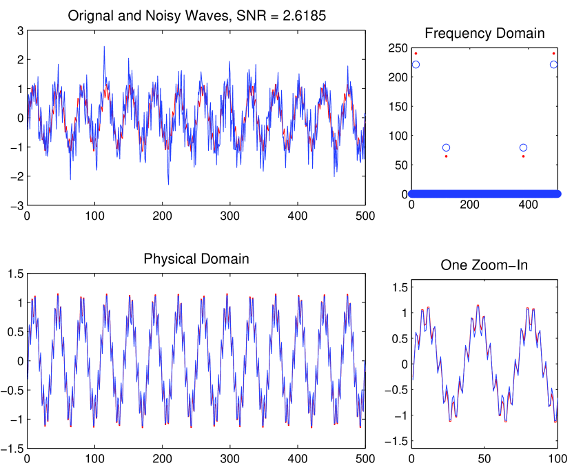
Figure 8: Reconstruction using 20% random samples of $\tilde{u}$ with SNR$=2.6185$. The upper left figure shows the original (red) and noisy (blue) signals; the upper right shows the reconstruction (blue circle) v.s. original signal (red dots) in Fourier domain in terms of their magnitudes (i.e. $|\widehat{u}^{*}|$ v.s. $|\widehat{\bar{u}}|$); bottom left shows the reconstructed (blue) v.s. original (red) signal in physical domain; and bottom right shows one close-up of the figure at bottom left.

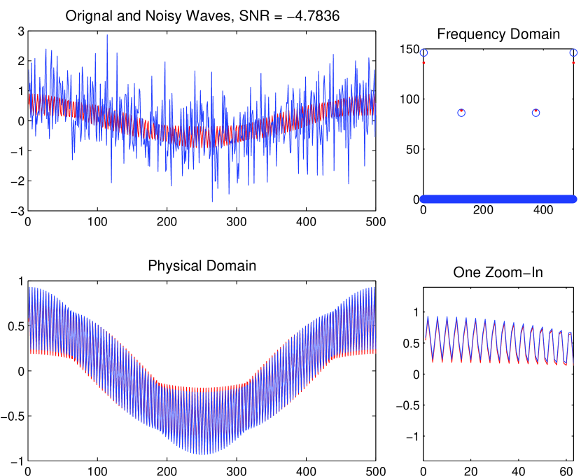
Figure 9: Reconstruction using 40% random samples of $\tilde{u}$ with SNR$=-4.7836$. The upper left figure shows the original (red) and noisy (blue) signals; the upper right shows the reconstruction (blue circle) v.s. original signal (red dots) in Fourier domain in terms of their magnitudes (i.e. $|\widehat{u}^{*}|$ v.s. $|\widehat{\bar{u}}|$); bottom left shows the reconstructed (blue) v.s. original (red) signal in physical domain; and bottom right shows one close-up of the figure at bottom left.

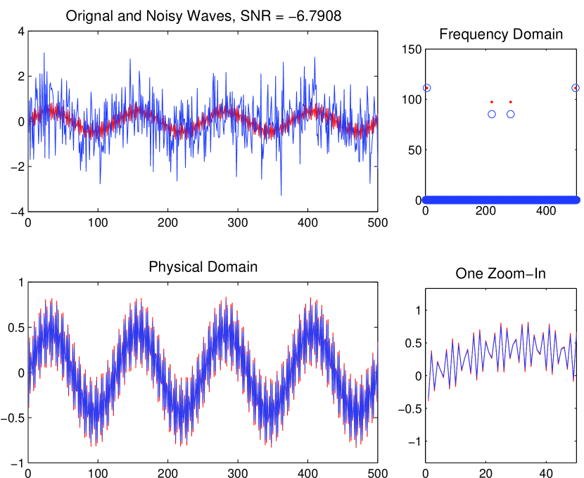
Figure 10: Reconstruction using 60% random samples of $\tilde{u}$ with SNR$=-6.7908$. The upper left figure shows the original (red) and noisy (blue) signals; the upper right shows the reconstruction (blue circle) v.s. original signal (red dots) in Fourier domain in terms of their magnitudes (i.e. $|\widehat{u}^{*}|$ v.s. $|\widehat{\bar{u}}|$); bottom left shows the reconstructed (blue) v.s. original (red) signal in physical domain; and bottom right shows one close-up of the figure at bottom left.

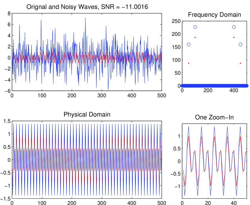
Figure 11: Reconstruction using 80% random samples of $\tilde{u}$ with SNR$=-11.0016$. The upper left figure shows the original (red) and noisy (blue) signals; the upper right shows the reconstruction (blue circle) v.s. original signal (red dots) in Fourier domain in terms of their magnitudes (i.e. $|\widehat{u}^{*}|$ v.s. $|\widehat{\bar{u}}|$); bottom left shows the reconstructed (blue) v.s. original (red) signal in physical domain; and bottom right shows one close-up of the figure at bottom left.

References

- [1] J. Darbon and S. Osher. Fast discrete optimizations for sparse approximations and deconvolutions. preprint 2007.
- [2] W. Yin, S. Osher, D. Goldfarb, and J. Darbon. Bregman iterative algorithms for compressed sensing and related problems. SIAM J. Imaging Sciences 1(1)., pages 143–168, 2008.
- [3] J. Cai, S. Osher, and Z. Shen. Linearized Bregman iterations for compressed sensing. Math. Comp., 2008. to appear, see also UCLA CAM Report 08-06.
- [4] J. Cai, S. Osher, and Z. Shen. Convergence of the linearized Bregman iteration for -norm minimization. UCLA CAM Report 08-52, 2008.
- [5] E. Candes, J. Romberg, and T. Tao. Robust uncertainty principles: exact signal reconstruction from highly incomplete frequency information. 52(2):489–509, 2006.
- [6] D.L. Donoho. Compressed sensing. IEEE Trans. Inform. Theory, 52:1289–1306, 2006.
- [7] S. Osher, M. Burger, D. Goldfarb, J. Xu, and W. Yin. An iterative regularization method for total variation based image restoration. Multiscale Model. Simul, 4(2):460–489, 2005.
- [8] E. Hale, W. Yin, and Y. Zhang. A fixed-point continuation method for -regularization with application to compressed sensing. CAAM Technical Report TR07-07, Rice University, Houston, TX, 2007.
- [9] L. Rudin, S. Osher, and E. Fatemi. Nonlinear total variation based noise removal algorithms. Phys. D, 60:259–268, 1992.
- [10] T-C. Chang, L. He, and T. Fang. Mr image reconstruction from sparse radial samples using bregman iteration. Proceedings of the 13th Annual Meeting of ISMRM, 2006.
- [11] Y. Li, S. Osher, and Y.-H. Tsai. Recovery of sparse noisy date from solutions to the heat equation. in preparation.
- [12] L.M. Bregman. The relaxation method of finding the common point of convex sets and its application to the solution of problems in convex programming. USSR Computational Mathematics and Mathematical Physics, 7(3):200–217, 1967.
- [13] D.L. Donoho. De-noising by soft-thresholding. IEEE Trans. Inform. Theory.
- [14] W. Yin. On the linearized bregman algorithm. private communication.
- [15] M. Bachmayr. Iterative total variation methods for nonlinear inverse problems. Master’s thesis, Johannes Kepler Universität, Linz, Austria, 2007.