Equation of State from Lattice QCD Calculations

Abstract

We provide a status report on the calculation of the Equation of State (EoS) of QCD at finite temperature using lattice QCD. Most of the discussion will focus on comparison of recent results obtained by the HotQCD and Wuppertal-Budapest (W-B) collaborations. We will show that very significant progress has been made towards obtaining high precision results over the temperature range of $T=150-700$ MeV. The various sources of systematic uncertainties will be discussed and the differences between the two calculations highlighted. Our final conclusion is that the lattice results of EoS are getting precise enough to justify being used in the phenomenological analysis of heavy ion experiments at RHIC and LHC.

1 The Road to Precision Lattice QCD Calculations

One of the goals of simulations of lattice QCD is to provide a precise non-perturbative determination of the EoS of QCD over the temperature range $150-700$ MeV that is being probed in experiments at RHIC and the LHC. The EoS, along with the transition temperature $T_{c}$ and transport coefficients such as shear viscosity, are crucial inputs into phenomenological hydrodynamical models used to describe the evolution of the quark gluon plasma (QGP). In this talk I will mainly review the two recent and most complete calculations of the EoS by the HotQCD [1] and Wuppertal-Budapest [2] collaborations.

Simulations of lattice QCD at finite temperature are carried out on a 4-D hypercube of size $aN_{\tau}\times aN_{S}\times aN_{S}\times aN_{S}$ where $a$ is the lattice spacing usually denoted in units of GeV^-1 or fermi. The spatial size $aN_{S}$ is taken large enough so that finite volume corrections are under control and small. Past calculations show that for finite temperature simulations with $N_{S}/N_{\tau}=4$ these corrections are smaller than statistical errors for $T\raise 1.29167pt\hbox{$<$\kern-7.5pt\raise-4.73611pt\hbox{$\sim$}}3T_{c}$. For higher temperatures larger $N_{S}$ may be required. In QCD, the gauge coupling $\beta\equiv 6/g^{2}$ is related to $a$ by dimensional transmutation and the continuum theory is recovered in the limit $a\to 0$ or equivalently $g\to 0$ or $\beta\to\infty$. To provide a perspective on how fine the current lattice simulations are note that $N_{\tau}=10$ corresponds to $a\approx 0.1$ fermi or $\sim 2$ GeV^-1 at the transition temperature $T\sim 200$ MeV.

The second set of control parameters (inputs) in the simulations are the quark masses. The results discussed in this review are for $2+1$ flavors, $i.e.$, two flavors of degenerate $u$ and $d$ quarks and a heavier strange quark. In nature $2m_{s}/(m_{u}+m_{d})\approx 27.5$ and $\overline{m}=(m_{u}+m_{d})/2\sim 3.5$ MeV and $m_{s}\sim 90$ MeV. The small value of $\overline{m}$ provides the key computational challenge because the most time consuming part of the simulations is the inversion of the Dirac operator, a very large sparse matrix. This inversion is done using interative Krilov solvers that have critical slowing down in the limit $\overline{m}\to 0$. The computational cost increases as $m^{-7/2}$ or faster and calculations become very expensive with decreasing quark mass. For this reason $2+1$ flavor simulations are typically done fixing the strange quark mass to its physical value and simulating at a number of values of $\overline{m}/m_{s}$ from which extrapolations to the physical $\overline{m}$ are made. Recent calculations by the W-B and HotQCD collaborations show that the computer power has reached a stage where simulations can be done close to, or directly at, physical $\overline{m}$. Thus, in the state-of-the-art simulations, this source of systematic error (extrapolation in $\overline{m}$) is now under good control.

The tuning of the set of parameters $\{g,m_{s},\overline{m}\}$ is done as follows. One first fixes the ratio $m_{s}/\overline{m}$, ideally to $m_{s}/\overline{m}=27.5$. Then for a judiciously chosen value of $g$, zero temperature simulations are done to measure two independent physical quantities whose values are experimentally measured or well determined, and one of which is sensitive to strange quark mass, for example the K-meson mass $M_{K}$ and the pion decay constant $f_{\pi}$ (or $f_{K}$ and $M_{\pi}$). The value of $m_{s}$ is tuned until the lattice results for these two quantities match their physical values. This fixes $a$ and $m_{s}$. Now depending on how finely one wants to scan in $T$ (or $a$) a new value of $g$ is chosen and the value of $m_{s}$ is again tuned to reproduce the observables, thus determining the new $a$ keeping $m_{s}/\overline{m}$ fixed. This process generates a set of $\{g,m_{s},\overline{m}\}$ values for which, by construction, the physics (defined by matching lattice $M_{K}$ and $f_{\pi}$ to physical values) is fixed. This line in the $\{g,m_{s},\overline{m}\}$ space, since $m_{s}$ is tuned to the physical value and $m_{s}/\overline{m}$ is fixed, is called a line of constant physics (LoCP). The utility of simulating along LoCP is to reduce the three dimensional space of input parameters to a line along which only the lattice spacing is changing. This procedure provides better control over taking the continuum limit. The extent to which $\{g,m_{s}\}$ would have varied had one chosen two different physical quantities, say $M_{\overline{s}s}$ and $M_{N}$, is a measure of variations in discretization errors along different LoCP. The emphasis of the lattice community is to present results extrapolated to $a\to 0$ in order to remove these discretization errors, which are proportional to powers of $a$, by simulating at a number of values of $a$. In case of finite temperature calculations we extrapolate results at fixed $T$ to $N_{\tau}\to\infty$ by simulating at a number of values of $N_{\tau}$.

The lattice size in the Euclidean time direction defines the temperature of the system by the relation $T=1/aN_{\tau}$. The scale $a$ for fixed $\{g,m_{s},\overline{m}\}$ is the same for zero-temperature and finite temperature lattices. Thus, knowing $a$ corresponding to a given $g$ and quark masses uniquely determines $T$ for a given $N_{\tau}$. An important consequence of the fact that $g$ or equivalently $a$ or $T$ is the single parameter that controls lattice simulations is that only one thermodynamic quantity can be determined, which for the extraction of EoS is the trace anomaly $I/T^{4}\equiv(\varepsilon-3p)/T^{4}$, where $I$ is called the integration measure.

The above approach for scanning in $T$ is called the fixed $N_{\tau}$ approach. A second approach that I will not cover in detail and which is being pursued by the WHOT collaboration [3] with improved Wilson fermions is called the fixed $a$ approach. In this approach, for a given $a$ (the same process is used for fixing $\{g,m_{s},\overline{m}\}$) one simulates on a number of different $N_{\tau}$ lattices to scan in $T$. The advantage of this approach is that only a single zero-temperature matching calculation, needed to carry out subtractions of lattice artifacts in finite $T$ data, is required for each $a$. The weakness of this approach is that the scan in $T$ is limited by the coarseness and range of $N_{\tau}$ values possible, $i.e.$ $N_{\tau}=6,8,10,12,14$, before one runs out of computational power. The recent results using the fixed $a$ approach by the WHOT collaboration [3] are very encouraging and I refer interested readers to their paper for details.

2 Taste Symmetry breaking with Staggerd fermions

In the naive discretization of the Dirac action there automatically is a $2^{4}$ doubling of flavors. In the staggered fermion approach, using a lattice symmetry called “spin diagonalization”, the degeneracy is reduced from 16 to 4 by placing a single degree of freedom at each lattice site. Under this construction a $2^{4}$ hypercube is the basic unit cell that reduces to a point in the continuum limit. The 16 degrees of freedom in the cell represent, in the continuum limit, four identical copies (called taste) of Dirac fermions. On the lattice this four-fold degeneracy gives rise to a proliferation of particles propagating in the QCD vacuum, for example, there are 16 pions distinguished by their taste rather than just one. If taste symmetry was unbroken at finite $a$, the 4-fold degeneracy could be handled by just dividing results by the appropriate degeneracy factor. Problems arise because this degeneracy is broken at finite $a$ and one does not know $a\ priori$ how large this systematic error is and how it effects simulations of QCD thermodynamics in particular. The most common approach to quantify this effect is to study the difference in the masses of the 16 pions, and determine how these differences vanish when lattice results are extrapolated to the continuum limit.

The HotQCD collaboration has studied the consequences of taste symmetry breaking utilizing three versions of improved staggered fermions $-$ the asqtad, p4 and HISQ/tree formulations [4]. In Fig. 1 we show preliminary HotQCD HISQ/tree results for $M^{2}_{\pi}-M^{2}_{G}$ where $M_{G}$ is the Goldstone pion mass versus $a$, and also compare with results from the stout and asqtad actions. The large spread in masses that increases on coarser lattices shows that taste symmetry is indeed badly broken [5]. Based on such studies the conclusion is that at any given $a$, the taste breaking is least in HISQ/tree followed by stout, asqtad, and p4 actions. One consequence of this discretization error for thermodynamics is that the contribution of any state, for example the pion, is not just from the lowest taste state (the Goldstone pion) but is some weighted average of the 16 pions (or the appropriate multiplets for other states). Thus, at any given $a$ the effective masses of all hadrons are larger than the desired ground state value. The magnitude of the effect is shown in the right panel of Fig. 1 which plots the root mean squared mass of the 16 pion states corresponding to a Goldstone pion mass of $140$ MeV. Results at low temperatures, $T<150$ MeV, and on small $N_{\tau}$ lattices are most susceptible to this discretization error. Taste breaking also puts a caveat on the above described tuning of quark masses: setting $m_{s}/\overline{m}=27.5$ does not guarantee that simulations have been done at the physical light quark masses. Simulating at a number of $m_{s}/\overline{m}$ values to control the chiral extrapolation followed by taking the continuum limit using a number of $N_{\tau}$ lattices provides the best understanding of systematic errors and for obtaining physical results.

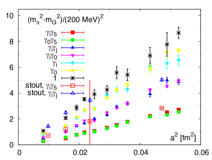
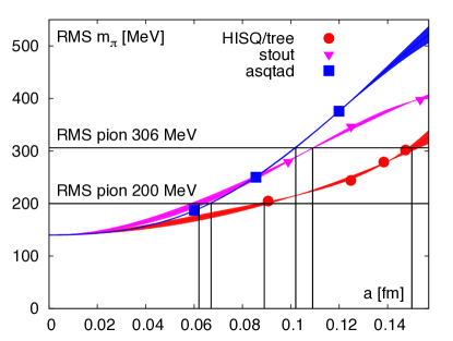
Figure 1: The splitting between the 16 pions due to taste symmetry breaking for HISQ/tree, stout and asqtad actions (left panel). The right panel shows the root mean squared mass corresponding to a Goldstone pion mass of $140$ MeV. Note that the HISQ action used so far for thermodynamics does not include tadpole improvement of the gauge action and is therefore called HISQ/tree in [4].

A second issue with staggered simulations that include the strange quark (or in future the charm quark) is the need to take the fourth root of the determinant to compensate for the 4-fold degeneracy. Creutz [6] claims that this “rooting” is a fundamental flaw of the staggered formulation, however, its effect in current simulations may be small since the strange quark mass is large, whereas the review by Sharpe [7] (covering a large body of work) shows that while the staggered formulation may be ugly, it gives physical results in the continuum limit. (For degenerate $u$ and $d$ quarks, this rooting problem is overcome because of a lattice symmetry whereby the square root of the determinant can be written as the determinant on even (or odd) sites.) In a perfect world one would like to use a Wilson-like action that maintains the continuum flavor structure and chiral symmetry, $i.e.$, domain wall or overlap fermions, however, to date most thermodynamical simulations use staggered fermions for two reason: they are much faster ($10-20\times$) to simulate than even simple Wilson fermions and because of a residual chiral symmetry that protects the Goldstone pion.

3 The Trace Anomaly

The results from the HotQCD [1] [4] and W-B [2] collaborations for $I/T^{4}\equiv(\varepsilon-3p)/T^{4}$, the single thermodynamic quantity calculated on the lattice, are shown in Fig. 2.

Before making detailed comparisons it is important to stress here, and applicable to all discussion that follows, that the HotQCD results do not yet incorporate extrapolation to the physical quark mass or the continuum limit. The most extensive data are for $N_{\tau}=6,8$ and $m_{s}/\overline{m}=10$ with new ongoing calculations at $m_{s}/\overline{m}=20$ and $N_{\tau}=12$. The W-B results at $N_{\tau}=6,8$ have been obtained for number of values of $m_{s}/\overline{m}$ including at $m_{s}/\overline{m}=28.15$ where the final physical value is quoted. (Recall, however, the caveat about the uncertainty in locating the physical value of $\overline{m}$ due to taste breaking.) The W-B data at $N_{\tau}=10$ and $12$ are more limited in $T$ values and are at $m_{s}/\overline{m}=28.15$ only. W-B define their $N_{\tau}=8$ results to represent the continuum value. Data with $N_{\tau}=10$ at $T\leq 365$ MeV (red points in left panel of Fig. 2) and the three points (green points in Fig. 2) with $N_{\tau}=12$ provide a consistency check since they show no significant discretization effects relative to $N_{\tau}=8$ data.

The overall form of the results by the two collaborations is similar. There are, however, two significant differences between the HotQCD and W-B data. The first is the value of $I$ at the peak, $\sim 5.8$ versus $4.1$, and the peak in the W-B data is shifted to lower $T$ by about $20$ MeV. W-B collaboration attribute these differences to the lack of extrapolation of HotQCD data in quark mass and $a$, $i.e.$, residual discretization errors. Preliminary HotQCD results with $N_{\tau}=8$ lattices using HISQ/tree fermions (also shown in Fig. 2) give a similar peak height and position as the asqtad action (the p4 results are higher but decreasing with $N_{\tau}$). The agreement between asqtad and HISQ/tree and since the HISQ/tree action is the more improved than stout, has smaller discretization errors and less taste breaking, it is not clear if, today, we have a simple resolution of the difference. The forthcoming results with HISQ/tree action on $N_{\tau}=8$ and $12$ lattices being simulated by the HotQCD collaboration should help clarify these issues.

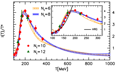
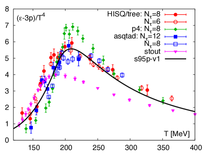
Figure 2: Integration measure $I/T^{4}$ from W-B (left) and preliminary HotQCD (right) comparing different actions. The curve (right panel) is a a parametrization of $\varepsilon-3p/T^{4}$ that is based on HRG and the p4/asqtad lattice data at high temperatures [8]; and the W-B data are shown in purple for comparison.

4 Pressure, Energy Density, Entropy and Speed of Sound

The pressure $p$ can be determined from the trace anomaly using the following relations:

$$\frac{I}{T^{4}}\equiv\frac{\Theta^{\mu\mu}(T)}{T^{4}} \equiv\frac{\varepsilon-3p}{T^{4}}=T\frac{\partial}{\partial T}\left(\frac{p}{T^{4}}\right)\,$$ (1)

$$\frac{p(T)}{T^{4}}-\frac{p(T_{0})}{T_{0}^{4}} =\int_{T_{0}}^{T}dt\frac{\Theta^{\mu\mu}(t)}{t^{5}}$$ (2)

The results for pressure and energy density are summarized in Figs. 3 and 4. To obtain pressure $p$ there are two issues that need to be addressed when carrying out the integration in Eq. 2. The first is to construct a smooth function that represents the lattice data for $(\varepsilon-3p)/T^{4}$ over the whole range of $T$ since $I/T^{4}$ has been calculated only at a finite number of values of $T$. The second is the choice of $T_{0}$ above which $\Theta^{\mu\mu}(T_{0})/T_{0}^{4}$ is well-determined and at which point $p(T_{0})$ can be estimated reliably.

The HotQCD collaboration has investigated a number of ansatz for parameterizing $\Theta^{\mu\mu}(T_{0})/T_{0}^{4}$ and find that the results for $p$ do not vary significantly. The uncertainty due to the ansatz is shown by the error bars on $p/T^{4}$ at $T=275,\ 540$ MeV in Fig. 3. The W-B collaboration uses a variant of the method $-$ they parameterize the pressure itself and then evaluate its derivatives to match to $I$. The band in Fig 4 show the uncertainty.

The second issue is more significant. The systematic errors in lattice data grow as $T$ is lowered and are expected to be large below $T=150$ MeV. At the same time $p(T=150)$ is not negligible and $a\ priori$ unknown. One approach is to use the hadron resonance gas (HRG) model for $p(T=150\ {\rm MeV})$. This requires that there be reasonable agreement between the HRG and lattice values at $T=150$ MeV. The HotQCD data approaches the HGR from below and at $T=150$ MeV there is a significant difference. Another approach is to use $T_{0}=100$ MeV where there is more confident in the HRG value but then one has to confront the uncertainty in matching and parameterizing $\Theta^{\mu\mu}(T_{0})/T_{0}^{4}$ between $T=100-150$ MeV. The HotQCD collaboration use $p=0$ at $T=100$ MeV for their central value and the HRG value to estimate the uncertainty whose magnitude is shown by the black square on $\varepsilon/T^{4}$ at $T=550$ MeV in Fig. 3. The W-B collaboration show that a modified “lattice” HRG calculation, taking into account taste breaking in pion and kaon states, fits the lattice data between $T=100-140$ MeV. Nevertheless, they choose $p(T=100MeV,m_{s}=\overline{m})=0$ for the normalization.

Once $I$ and $p$ are determined the energy density is given by $\varepsilon/T^{4}=I/T^{4}+3p/T^{4}$, entropy by $s=(\varepsilon+p)/T$ and the speed of sound $c_{s}$ by

$$c_{s}^{2}=\frac{dp}{d\varepsilon}=\varepsilon\frac{d(p/\varepsilon)}{d\varepsilon}+\frac{p}{\varepsilon}\;\;.$$ (3)

A comparison of results for $\varepsilon$, $p$ and $s$ is shown in Figures 3, 4, and 5.

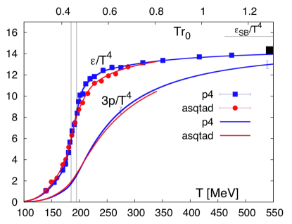
Figure 3: HotQCD collaboration [1] results for $\varepsilon/T^{4}$ and $3p/T^{4}$ on $N_{\tau}=8$ lattices with $m_{s}/\overline{m}=10$.

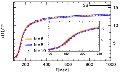
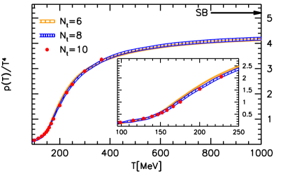
Figure 4: Results for $\varepsilon/T^{4}$ and $p/T^{4}$ from the W-B collaboration [2]. To compare results for $p$ note that the W-B data are for $p/T^{4}$ whereas the HotQCD results in Fig 3 are for $3p/T^{4}$.

The W-B collaboration apply two corrections to the estimate for $p(T)$. The first is to guarantee that the lattice results for each $N_{\tau}$ match the continuum Stefan-Boltzmann value at $T=\infty$. To do this they construct the ratio of the continuum Stefan-Boltzmann value for $p$ to its free-field ($T=\infty$) lattice value (the continuum integrals are replaced by lattice sums appropriate for each $N_{\tau}$) and then correct the lattice data at all $T$ by this ratio. This ratio is large, $1.517$ and $1.283$ for $N_{\tau}=6$ and $8$ respectively. Since $N_{\tau}=8$ data are used to define the continuum estimate, this correction is too large to justify on the basis of a tree-level improvement of lattice observables (lattice operators used to probe the physics). Furthermore, this correction is also applied to $I$, $\varepsilon$ and $s$. The second correction made by the W-B collaboration is to shift upward their results for $p/T^{4}$ by half the difference, $0.06$, between the lattice and HRG estimates at $T=100$ MeV. Again, to me, this is not a well-motivated correction of data. Future simulations and better understanding of the low $T$ region will hopefully alleviate the need for such corrections.

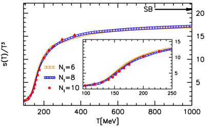
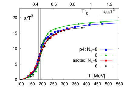
Figure 5: Comparison of entropy density obtained by W-B (left) and HotQCD (right) collaborations. The HotQCD data are for $m_{s}/\overline{m}=10$.

A comparison of results for the speed of sound are shown in Fig. 6. The fundamental quantity needed to calculate it is ${p/\varepsilon}$ as shown in Eq. 3. Two features in the data are worth commenting on. First, data in Fig. 4 show that, in the transition region from hadronic matter to QGP, the energy density is changing more rapidly than the pressure. This implies that $c_{s}$ should show a dip in the transition region as is indeed observed. Second, $c_{s}$ rises quickly after the transition region and reaches close to the relativistic Boltzmann gas value of $1/3$ by $T\sim 400$ MeV.

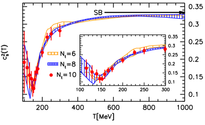
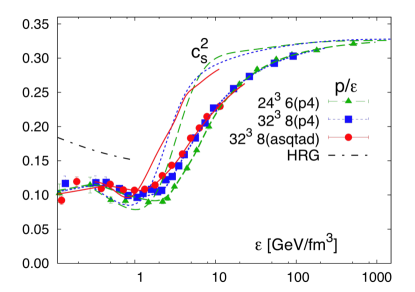
Figure 6: Comparison of the speed of sound $c_{s}^{2}$. The W-B data (left panel) are plotted versus $T$. The HotQCD data for $p/\varepsilon$ and $c_{s}^{2}$ versus the energy density $\varepsilon$ using the fits to $\varepsilon$ and $p$ (right panel).

5 Prospects for improvement in the EoS of QCD in the near future

Significant progress has been made in determining the EoS using lattice QCD in the last three years. The current lattice results for the EoS have already given the Heavy Ion community a much better understanding of the dynamics of the QGP. Lattice estimates are now being used in hydrodynamic analysis of the evolution of the QGP in experiments at the RHIC at BNL and at the LHC.

There are a number of ways in which both HotQCD and W-B collaborations are improving their estimates:

• The HotQCD collaboration will present their estimates of the continuum values with HISQ/tree action on $N_{\tau}=6,\ 8$ and $12$ lattices and with $m_{s}/\overline{m}=10$ and $20$.

• Both collaborations will include the charm quark to provide results with ($2+1+1$) dynamical flavors. Preliminary partially-quenched estimates suggest that the charm quark contribution starts to become large at above $T\sim 300$ MeV.

• To fully control finite volume effects at $T>500$, both collaborations will simulate on larger spatial volumes, larger than $N_{s}/N_{\tau}=4$.

• In addition to simulations with staggered fermions, simulations with improved Wilson and domain wall fermions are maturing [3] [9] and will provide independent checks of the staggered results in, hopefully, the near future.

With these improvements a number of unresolved issues such as the location and height of the peak in $I$, control over systematic errors at low temperatures, and the impact of charm quark at high temperatures, should be addressed over the next couple of years. So stay tuned.

Acknowledgements: I thank T. Nayak, R. Verma and P. Ghosh for the invitation to a very informative conference and acknowledge the support of DOE grant KA140102.

References

- [1] A. Bazavov et al. [HotQCD Collaboration], Phys.Rev.D80:014504,2009 [arXiv:0903.4379].
- [2] S. Borsanyi et al. [Wuppertal-Budapest Collaboration] JHEP11(2010)077 [arXiv:1007.2580].
- [3] T. Umeda et al. [WHOT Collaboration] [arXiv:1011.2548].
- [4] A. Bazavov, P. Petreczky [HotQCD Collab.], [arXiv:1012.1257], and C. DeTar [arXiv:1101.0208].
- [5] E. Follana [HPQCD and UKQCD collaborations], Phys. Rev. D75 (2007) 054502.
- [6] M.Creutz, PoS LATTICE2007, 007 (2007) [arXiv:0708.1295]
- [7] S.R.Sharpe, PoS LATTICE2006, 022(2006)[arXiv:hep-lat/0610094]
- [8] P. Huovinen, P. Petreczky, Nucl. Phys. A837, 26-53 (2010). [arXiv:0912.2541 [hep-ph]].
- [9] M. Cheng , Phys.Rev.D81:054510,2010 [arXiv:0911.3450]