Ultra High Energy Cosmic Rays Propagation and Spectrum

Abstract

The status of the observations of Ultra High Energy Cosmic Rays will be reviewed, focusing on the the latest results of HiRes and Auger observatories. A comprehensive analytical computation scheme to compute the expected UHECR spectrum on earth will be presented, applying such scheme to interpret the experimental results. The phenomenological scenarios favored by HiRes and Auger in terms of chemical composition and spectrum will be also presented.

1 Introduction

Ultra High Energy Cosmic Rays (UHECR) are the most energetic particles observed in nature with energies up to $3\times 10^{20}$ eV. The detection of these particles, started already in the 50s with the pioneering experiments of Volcano Ranch in the USA and Moscow University array in the USSR, poses many interesting questions mainly on the origin and chemical composition of such fascinating particles. In the recent years a new step forward was done with the measurements performed by HiRes and AGASA first, and nowadays with the first five years results of the Pierre Auger Observatory in Argentina.

The propagation of UHECR from the sources to the observer is mainly conditioned by the interaction of these extremely energetic particles with the intervening astrophysical backgrounds such as the Cosmic Microwave Background (CMB) and the Extraglactic Background Light (EBL). The study of the propagation of UHE particles through these backgrounds is of paramount importance to interpret the observations and to discover the astrophysical origin of UHECR. Several propagation dependent features in the spectrum can be directly linked to the chemical composition of UHECR and/or to the distribution of their sources GZK ; dip ; AloBon . Among such features particularly important is the Greisin, Zatsepin and Kuzmin (GZK) suppression of the flux GZK , an abrupt depletion of the observed proton spectrum due to the interaction of the UHE protons with the CMB radiation field. The GZK suppression, as follows from the original papers GZK , is referred to protons and it is due to the photo-pion production process on the CMB radiation field ($p+\gamma_{CMB}\to\pi+p$). In the case of nuclei the expected flux also shows a suppression at the highest energies that, depending on the nuclei specie, is due to the photo-disintegration process on the CMB and EBL radiation fields ($A+\gamma_{CMB,EBL}\to(A-nN)+nN$). In any case, the interaction processes between UHE particles and astrophysical backgrounds will condition the end of the CR spectrum at the highest energies and the high energy behavior of the flux can be used as a diagnostic tool for the chemical composition of the observed particles. Another important feature in the spectrum that can be directly linked with the nature of the primary particles and on their origin (galactic/extra-galactic) is the pair-production dip dip . This features is present only in the spectrum of UHE extragalactic protons and, as the GZK, is a direct consequence of the proton interaction with the CMB radiation field, in particular the dip brings a direct imprint of the pair production process $p+\gamma_{CMB}\to p+e^{+}+e^{-}$ suffered by protons in their interaction with CMB radiation.

From the experimental point of view the situation is far from being clear with different experiments claiming contradictory results. The HiRes experiment shows a proton dominated spectrum till the highest energies with a clear observation of the protons GZK suppression and the pair-production dip HiRes . The chemical composition observed by HiRes is coherent with this picture showing a proton dominated spectrum at all energies $E>10^{18}$ eV HiRes . The situation changes if the Auger results are taken into account. The latest release of the observed Auger spectrum Auger shows a not clear confirmation of the pair production dip and of the protons GZK suppression. Signaling a possible deviation from a proton dominated spectrum to an heavier composition at the highest energies. This picture is confirmed by the chemical composition observed by Auger, that shows an heavy mass composition at energies $E>4\times 10^{18}$ eV Auger .

This puzzling situation, with different experiments favoring different scenarios, shows the importance of a systematic study of UHECR propagation in astrophysical backgrounds. In the present paper we will review the main points of the kinetic theory of UHECR propagation, comparing theoretical results with the latest experimental data of Auger ad HiRes. The paper is organized as follows: in section 2 we review the kinetic theory of propagation for protons and nuclei, in section 3 we will discuss different theoretical scenarios in comparison with experimental data, conclusions will take place in section 4.

2 Protons and Nuclei Propagation

The propagation of charged particles (protons or nuclei) in astrophysical backgrounds can be suitably studied in the kinetic approach, that enables the computation of the expected fluxes on earth given any hypothesis on the astrophysical sources of UHECR. The main assumption under which the kinetic theory is build is the Continuum Energy Losses (CEL) approximation BereBook , through which particle interactions are treated as a continuum process that continuously depletes the particles energy.

In the propagation through astrophysical backgrounds the interactions of particles are naturally affected by fluctuations, with a non-zero probability for a particle to travel without loosing energy. In our computation scheme such fluctuations are neglected; as was shown in dip ; BereKach this approach has a limited effect on the flux computation. Only at the highest energies ($E>100$ EeV) fluctuations produce a deviation of the order of $10\%$ respect to the flux computed with a standard Monte Carlo simulation BereKach .

As already anticipated in the introduction UHECR propagating through astrophysical backgrounds suffer different interaction processes loosing energy and, in the case of nuclei, being even destroyed.

• protons - UHE protons interact only with the CMB radiation field giving rise to the two processes of pair production and photo-pion production. Both of these reactions can be treated in the CEL hypothesis.

• nuclei - UHE nuclei interact with the CMB and EBL radiation fields, suffering the process of pair production, for which only CMB is relevant, and photo-disintegration, that involves both backgrounds CMB and EBL. While the first process can be treated in the CEL hypothesis, being the nuclei specie conserved, the second produces a change in the nucleus specie. Following AloBere10 we will treat the photo-disintegration process as a ”decaying” process that simply depletes the flux of the propagating nucleus.

The propagation of UHE particles in the energy range $E\simeq 10^{18}\div 10^{19}$ eV is extended over cosmological distances with a typical path length of the order of Gpc. Therefore we should also take into account the adiabatic energy losses suffered by particles because of the cosmological expansion of the Universe.

The kinetic equation that describes the propagation of protons and nuclei are respectively:

$$\frac{\partial n_{p}(\Gamma,t)}{\partial t}-\frac{\partial}{\partial\Gamma}\left[b_{p}(\Gamma,t)n_{p}(\Gamma,t)\right]=Q_{p}(\Gamma,t)$$ (1)

$$\frac{\partial n_{A}(\Gamma,t)}{\partial t}-\frac{\partial}{\partial\Gamma}\left[n_{A}(\Gamma,t)b_{A}(\Gamma,t)\right]+\frac{n_{A}(\Gamma,t)}{\tau_{A}(\Gamma,t)}=Q_{A}(\Gamma,t)$$ (2)

where $n$ is the equilibrium distribution of particles, $b$ are the energy losses (adiabatic expansion of the Universe and pair/photo-pion production for protons or only pair-production for nuclei) $Q$ is the injection of freshly accelerated particles and, in the case of nuclei, also the injection of secondary particles produced by photo-disintegration (see below).

Concerning sources, in this paper, we will consider the simplest hypothesis of a uniform distribution of sources that inject UHECR of different species with a power law injection of the type:

$$Q_{inj}(\Gamma,z)=Q_{0}(z)\Gamma^{-\gamma_{g}}e^{-\Gamma/\Gamma_{max}}$$ (3)

where $\Gamma$ is the Lorentz factor of the particle, $\Gamma_{max}$ is the maximum Lorentz factor that the sources can provide and $\gamma_{g}$ is the power law index of the distribution of the accelerated particles at the sources. In our discussion, depending on the particle specie, we will consider different injection parameters $Q_{0}$ and $\Gamma_{max}$, keeping the power law index $\gamma_{g}$ fixed for all species.

The energy losses $b$ for protons or nuclei depend only on the CMB field and in the CEL hypothesis can be computed analytically through dip :

$$b(\Gamma)=\frac{c}{2\Gamma}\int_{\epsilon_{0}}d\epsilon_{r}\sigma(\epsilon_{r})f(\epsilon_{r})\epsilon_{r}\int_{\epsilon_{r}/2\Gamma}d\epsilon\frac{n_{CMB}(\epsilon)}{\epsilon^{2}}$$ (4)

where $\Gamma$ is the Lorentz factor of the UHE particle, $\epsilon_{r}$ is the energy of the background photon in the rest frame of the UHE particle, $\epsilon_{0}$ is the threshold of the considered reaction in the rest system of the UHE particle, $\sigma(\epsilon_{r})$ is the cross-section of the process, $f(\epsilon_{r})$ is the mean fraction of energy lost by UHE particle in a single collision in the laboratory system, and $n_{CMB}(\epsilon)$ is the density of the CMB background photons in the Laboratory reference frame.

The energy losses (4) do not take into account the expansion of the Universe and are intended at the present epoch $(z=0)$, in order to generalize energy losses at any red-shift $z$, because in the computation of $b$ only CMB plays a role, one can simply use the following recipe $b(\Gamma,z)=(1+z)^{2}b((1+z)\Gamma,z=0)$. The expansion of the universe is taken into account by adding $b(\Gamma,z)+\Gamma(1+z)H(z)$, with $H(z)=H_{0}\sqrt{(1+z)^{3}\Omega_{m}+\Omega_{\Lambda}}$. In the present paper we will always assume standard cosmology with $H_{0}=72$ Km/(s Mpc), $\Omega_{m}=0.27$ and $\Omega_{\Lambda}=0.73$.

In figure 1 we show the behavior of the path-length $\lambda=c/b_{p}$ (at $z=0$) for protons, from the figure it is evident the effect of the photo-pion production process with a sharp decrease of the contributing Universe that is at the basis of the expected GZK cut-off in the proton spectrum.

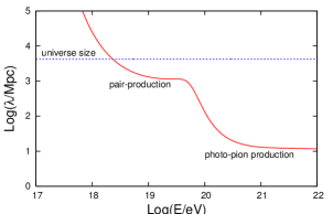
Figure 1: protons path length, with labels of the relevant process that fix the behavior in different energy regimes. The sharp suppression of the path length responsible of the expected GZK cut-off is clearly seen as a consequence of the photo-pion production process. Only the CMB radiation field is relevant for proton propagation (see the text).

In the case of nuclei the energy losses term $b_{A}$ in equation (2) depends only on the pair-production process on CMB and on the universe expansion. The rate $b_{A}$ can be computed as in equation (4) and it is easy to show that it is related to the protons pair-production loss rate by the relation:

$$b_{A}(\Gamma)=\frac{Z^{2}}{A}b_{b}(\Gamma)$$ (5)

where $Z,A$ are the charge (atomic number) and atomic mass number of the nucleus. The second process that affects nuclei propagation is photo-disintegration over CMB and EBL backgrounds. This process is treated as a decaying process that depletes the flux of nuclei, it enters in the kinetic equation (see equation (2)) through a sort of ”life-time” of the nucleus under the photo-disintegration process. This ”life-time” corresponds to the mean time needed to a nucleus of Lorentz factor $\Gamma$ and atomic number $A$ to lose, at least, one of its nucleons:

$$\frac{1}{\tau_{A}}=\frac{c}{2\Gamma^{2}}\int_{\epsilon_{0}(A)}^{\infty}d\epsilon_{r}\sigma(\epsilon_{r},A)\nu(\epsilon_{r})\epsilon_{r}\int_{\epsilon_{r}/(2\Gamma)}^{\infty}d\epsilon\frac{n_{bkg}(\epsilon)}{\epsilon^{2}}$$ (6)

where $\sigma(\epsilon_{r},A)$ is the photo-disintegration cross-section and $\nu(\epsilon_{r})$ is the molteplicity associated to this process, namely the average number of nucleons extracted from the nucleus by a single interaction and $n_{bkg}=n_{CMB}+n_{EBL}$. The dependence on red-shift of $\tau_{A}$ directly follows from the evolution with red-shift of the background photon densities $n_{CMB}$ and $n_{EBL}$. In the case of CMB this dependence is known analytically while for the EBL we will refer to the models presented by Stecker Stecker_EBL . In figure 2 we show the behavior of the path length $\lambda$ for different nuclei species, being $\lambda=c/b_{A}$, for pair-production, or $\lambda=c\tau_{A}$, for photo-disintegration. In figure 2 we show also the effect of the EBL by plotting $\lambda$ computed taking into account both backgrounds (continuos line) and only CMB (black dotted line). It is important to note that the photo-disintegration process starts to contribute to the propagation of nuclei at a Lorentz factor that is almost independent of the nuclei specie $\Gamma_{cr}\simeq 2\times 10^{9}$ AloBere10 . This is an important general characteristic of nuclei photo-disintegration process from which we can immediately deduce the dependence on the nucleus specie of the energy corresponding to the photo-disintegration suppression of the nuclei flux:

$$E^{A}_{cut}=Am_{N}\Gamma_{cr}$$ (7)

being $A$ the atomic number of the nucleus and $m_{N}$ the proton mass. From equation (7) it is evident how the flux behavior could bring informations on the chemical composition of the UHECR, in the case of Helium ($A=4$) the suppression is expected around energies $E\simeq 10^{19}$ eV while in the case of Iron ($A=56$) the suppression is expected at higher energies $E\simeq 10^{20}$ eV.

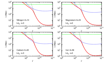
Figure 2: Nuclei path length under the processes of pair production $\lambda=c/b_{A}$ (blue dotted) and photo-disintegration $\lambda=c\tau_{A}$. In the case of photo-disintegration we have considered the path-length computed taking into account all relevant backgrounds CMB and EBL (red continuos line) and only CMB (black dotted line). The size of the Universe is also shown as greed dashed line.

Let us discuss now the generation function $Q_{A}(\Gamma,t)$ in the rhs of Eq. (2). One should distinguish among primary nuclei, i.e. nuclei accelerated at the source and injected in the intergalactic space, and secondary nuclei and protons, i.e. particles produced as secondaries in the photo-disintegration chain. In the case of primaries the injection function has the form (3), while the injection of secondaries should be modeled taking into account the characteristics of the photo-disintegration process. The dominant process of photo-disintegration is the one nucleon ($N$) emission, namely the process $(A+1)+\gamma_{bkg}\to A+N$, this follows directly from the behavior of the photo-disintegration cross-section (see AloBere10 and references therein) that shows the giant dipole resonance corresponding to one nucleon emission. Moreover, at the typical energies of UHECR ($E>10^{17}$ eV) one can safely neglect the nucleus recoil so that photo-disintegration will conserve the Lorentz factor of the particles. Therefore the production rate of secondary $A-$nucleus and $A-$associated nucleons will be given by

$$Q_{A}(\Gamma,z)=Q_{p}^{A}(\Gamma,z)=\frac{n_{A+1}(\Gamma,z)}{\tau_{A+1}(\Gamma,z)}$$ (8)

where $\tau_{A+1}$ is the photo-disintegration life-time of the nucleus father $(A+1)$ and $n_{A+1}$ is its equilibrium distribution, solution of the kinetic equation (2).

Using equation (8) we can build a system of coupled differential equations that starting from primary injected nuclei $(A_{0})$, with an injection given by (3), follows the complete photo-disintegration chain for all secondary nuclei $(A<A_{0})$ and nucleons. Clearly secondary protons propagation will be described by the proper kinetic equation (1) with an injection term given by (8). The solution of the kinetic equation for protons and nuclei can be worked out analytically. In the case of protons:

$$n_{p}(\Gamma,z)=\int_{z}^{z_{max}}\frac{dz^{\prime}}{(1+z^{\prime})H(z^{\prime})}Q_{p}(\Gamma^{\prime},z)\frac{d\Gamma^{\prime}}{d\Gamma}$$ (9)

being $Q_{p}$ the injection of primary protons (equation (3)) or secondary protons (equation (8)) and $\Gamma^{\prime}=\Gamma^{\prime}(\Gamma,z)$ is the characteristic function of the kinetic equation AloBere10 . In the case of nuclei:

$$n_{A}(\Gamma,z)=\int_{z}^{z_{max}}\frac{dz^{\prime}}{(1+z^{\prime})H(z^{\prime})}Q_{A}(\Gamma^{\prime},z)\frac{d\Gamma^{\prime}}{d\Gamma}e^{-\eta_{A}(\Gamma^{\prime},z^{\prime})}.$$ (10)

being, again, $Q_{A}$ the injection of primary nuclei (3) or secondary (8). The exponential term in Eq. (10) is given by

$$e^{-\eta_{A}(\Gamma^{\prime},z^{\prime})}=\exp\left[-\int_{z}^{z^{\prime}}\frac{dz^{\prime\prime}}{(1+z^{\prime\prime})H(z^{\prime\prime})}\frac{1}{\tau_{A}(\Gamma^{\prime\prime},z^{\prime\prime})}\right],$$ (11)

in which one easily recognizes the survival probability during the propagation time $t^{\prime}-t$ for a nucleus with fixed $A$. Therefore, $\exp(-\eta)$ provides the suppression of large $z^{\prime}$ in the integral in Eq. (10). The derivative term $d\Gamma^{\prime}/d\Gamma$ present in both solutions (9) and (10) can be computed according to AloBere10 . Finally, the maximum red-shift of integration $z_{max}$ can be directly computed solving the equation $\Gamma^{\prime}(\Gamma,z)=E_{max}$, assuming a maximum acceleration energy $E_{max}=Am_{N}\Gamma_{max}$ ($A=1$ for protons) in the injection of freshly accelerated particles.

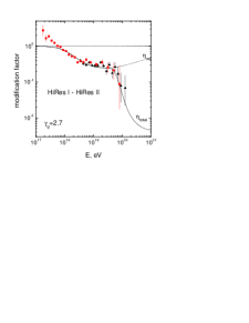
Figure 3: Pure proton spectrum in comparison with HiRes data HiRes , data are from HiRes II monocular (boxes) and HiRes I monocular (triangles). The two curves $\eta_{tot}$ and $\eta_{ee}$ show the total spectrum and the spectrum calculated including only adiabatic and pair-production energy losses.

3 Comparison with Observations

Using the solutions of the kinetic equation (9) and (10) we can compute the expected flux on earth (at $z=0$). In this section we will discuss the two alternative scenarios that follows from the observations of Auger and HiRes. Let us first consider the case of HiRes data. In figure 3 we show the comparison of these data with a pure proton spectrum, the comparison is performed by means of the modification factor $\eta(E)$ dip . This quantity is given by the ratio of the energy spectrum $n_{p}(E)$ calculated from equation (9) (with all energy losses taken into account), and the unmodified spectrum $n_{unm}(E)$, where only adiabatic energy loss (Universe expansion) is included: $\eta(E)=n_{p}(E)/n_{unm}(E)$ dip . The modification factor is a convenient quantity to describe, in a model independent way dip , any feature in the spectrum related to energy losses. From figure 3 it is evident the agreement of the HiRes observed spectrum with the expected pair production dip, typical of a pure proton spectrum with a best fit injection power law $\gamma_{g}=2.7$ dip .

The nature of the spectrum suppression seen in figure 3 can be further characterized taking the integral spectrum as observed by HiRes. The GZK suppression for protons in the integral spectrum can be tagged by the energy scale $E_{1/2}$, that corresponds to the energy at which the integral spectrum $J(>E)$ becomes half of the simple power-law extrapolation spectrum $KE^{-\gamma}$. Theoretical calculations for protons predict a value $E_{1/2}=10^{19.72}$ eV for a wide range of injection power laws $\gamma_{g}=2.1\div 2.8$ BereE1/2 . The measured value of $E_{1/2}$ as claimed by the HiRes collaboration is in fairly good agreement with the predicted value, being $E_{1/2}^{HiRes}=10^{19.73\pm 0.07}$. From these observations of HiRes, with some caution, one may conclude that HiRes has detected the two main signatures of a pure proton composition: the pair production dip and the GZK suppression. This important conclusion of the HiRes observations is confirmed from the direct measurement of the UHECR chemical composition performed by this experiment. In particular, the HiRes measurement of the elongation rate $X_{max}$ and its root-mean-square (RMS) confirm a strong dominance of protons in the UHECR composition at all energies $E>10^{18}$ eV HiRes .

The picture emerging from HiRes observations is not confirmed by Auger. The Auger data on mass composition and spectra are quite different from those of HiRes. In particular, the Auger observations show a nuclei dominated spectrum already at energies around $4\times 10^{18}$ eV. This conclusion is quite robust in the Auger data and it follows from both observations on elongation rate as well as on its RMS. The change with energy of mass composition in the Auger data is quite smooth with a progressive increase of the heavy nuclei content starting already at $2\times 10^{18}$ eV.

Coherently with the elongation rate observations the UHECR flux observed by Auger is difficult to reconcile with a pure proton spectrum. In figure 4 we show the comparison of the Auger spectrum with a pure proton spectrum obtained fixing the injection power law $\gamma_{g}=2.8$ and with different choices of the maximum attainable energy at the source (as labeled). It is clear that the observed spectrum is well described by a pure proton flux only at energies below $(3\div 5)\times 10^{18}$ eV. At larger energies the theoretical proton spectrum is not compatible with the Auger observations disapp , that don’t show the typical dip behavior as discussed in the case of HiRes data. The same conclusion holds changing the injection power law, taking a very flat injection with $\gamma_{g}=2.0$ the situation doesn’t change with the theoretical proton spectrum compatible with Auger observations only at low energy, $E<(3\div 5)\times 10^{18}$ disapp .

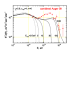
Figure 4: Pure proton spectrum with an injection power law $\gamma_{g}=2.8$ and for different choices of the maximum energy $E_{max}$ (as labelled) in comparison with the observed Auger flux.

As discussed in the case of HiRes observations, another important signature of the proton content at the highest energies is related to the shape of the flux suppression. Also under this respect the flux observed by Auger seems not compatible with a pure proton composition. The value of $E_{1/2}$ and the behavior of the suppression are better related to an heavy nuclei composition than a pure proton.

As recently pointed out in disapp , the experimental evidence emerging from Auger data can be understood in terms of different primary species and their maximum energy at the source. A large set of astrophysical acceleration mechanisms, in particular those based on diffusive shocks, show a maximum energy at the source which is rigidity dependent, being related to the electric charge of the accelerated particle: $\Gamma^{A}_{max}\propto Z\Gamma^{p}_{max}$ with $\Gamma^{A}_{max}$ maximum Lorentz factor of a nucleus with atomic number $Z$ and $\Gamma^{p}_{max}$ maximum Lorentz factor for protons. Using this characteristic of the maximum energy it is possible to explain the progressively heavier composition with increasing energy observed by Auger. This goal is reached by the so-called ”disappointing model” disapp , that describes the Auger observations by means of a multi-component injection of UHECR at the sources. At energy higher than $ZE_{max}^{p}$ nuclei with charge $Z^{\prime}<Z$ disappear, while heavier nuclei with larger Z survive. Starting from $E^{p}_{max}\simeq(4\div 10)\times 10^{18}$ eV, the higher energies are accessible only for nuclei with progressively larger values of $Z$. In particular, the maximum observed energy must correspond to Iron nuclei, which can reach $E_{max}^{Fe}\simeq(1\div 3)\times 10^{20}$ eV. In figure 5 we plot the UHECR spectrum in a two component model: protons and Iron, in comparison with the Auger observed flux, for an injection power law index $\gamma_{g}=2.0$ and a value of the maximum energy for protons of $E_{max}^{p}=4\times 10^{18}$ eV. From this figure it is evident the good agreement of this simple (two-components) model with the Auger observations. The predictions of this model are very disappointing for future detectors. In fact, the maximum energy for Iron $E_{max}^{Fe}=(1\div 4)\times 10^{20}$ eV implies an energy per nucleon below the threshold $E_{N}<E_{max}^{Fe}/A\simeq(2\div 5)\times 10^{18}$ eV, i.e. well below the GZK energy. Therefore, the production of secondary detectable particles such as neutrinos or gamma-rays will be subdominant respect to the photo-disintegration process of nuclei and no alternative detection of the UHECR propagation will be possible disapp . Moreover, it will be impossible any correlation study of the UHECR events with possible astrophysical sources because the effect of galactic magnetic field will substantially deviate the nuclei trajectories at the highest energies disapp . For these reasons the model at hand, while gives a good description of the Auger observations, was named ”disappointing” by the authors of disapp .

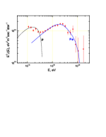
Figure 5: UHECR spectrum in a two component model with protons and Iron nuclei, the injection power law index is $\gamma_{g}=2.0$ and the maximum energy is $E_{max}=4Z\times 10^{18}$ eV.

4 Conclusions

In conclusion, we face at present the most serious disagreement in the observational data of the two biggest experiments in UHECR. HiRes observes signatures of proton propagation through CMB in the form of the pair-production dip and GZK cutoff. Moreover, these observations are well confirmed by the HiRes direct measurement of a proton dominated mass composition. The study of UHECR propagation enables us to accommodate HiRes observations in a pure proton model, with sources characterized by a steep injection spectrum $\gamma_{g}=2.5\div 2.8$ and an high maximum energy $E_{max}^{p}=(1\div 3)\times 10^{20}$ eV.

On the other hand, Auger clearly observes an high-energy steepening of the spectrum, but its position and shape are rather different from the prediction of the GZK cutoff. Moreover, the behavior of the spectrum observed by Auger in the energy range $1\times 10^{18}\div 4\times 10^{19}$ eV doesn’t confirm the pair-production dip typical of protons, signaling a substantial nuclei contamination in the flux observations. Coherently with this, the mass composition directly observed by Auger at $E\geq 4\times 10^{18}$ eV shows a dominance of nuclei that becomes progressively heavier increasing the energy and reaches a pure Iron composition at $E\simeq 10^{19}$ eV.

From our analysis follows that the Auger data favor a multi-component spectrum at the sources with a conservative explanation in terms of flat injection $\gamma_{g}=2.0\div 2.3$ and a relatively low maximum energy for protons $E_{max}^{p}\simeq(3\div 5)\times 10^{18}$ eV, that corresponds to a maximum energy for Iron nuclei of the order of $E_{max}^{Fe}\simeq(1\div 2)\times 10^{20}$ eV. This scenario emerging from Auger observations, if confirmed, will be quite disappointing because the dominance of nuclei at the highest energies will seriously harm any experimental study of correlation with sources as well as any detection of UHE neutrinos or gamma-rays produced by UHECR propagation.

Let us conclude by stating that the experimental observation of the UHECR chemical composition at the highest energies has a paramount importance in choosing among the two alternative scenarios depicted in this paper and establishing the future directions of this field of research. Unfortunately the available observations at the highest energies are still affected by poor statistics and renewed experimental efforts are needed in order to unveil the nature of UHECR.

References

- (1) K. Greisen, Phys. Rev. Lett. 16, 748 (1966); G.T. Zatsepin and V.A. Kuzmin, Pisma Zh. Experim. Theor. Phys. 4, 114 (1966).
- (2) V. Berezinsky, A. Gazizov and S. Grigorieva, Phys. Rev. D 74, 043005 (2006); R. Aloisio, V. Berezinsky, P. Blasi, A. Gazizov, S. Grigorieva and B. Hnatyk, Astrop. Phys. 27, 76 (2007).
- (3) R. Aloisio and D. Boncioli, arXiv:1002.4134 [astro-ph.HE].
- (4) HiRes collaboration, Phys. Rev. Lett. 100 (2008) 101101; P. Sokolsky, arXiv:1010.2690 [astro-ph.HE]; HiRes collaboration, Phys. Rev. Lett. 104 (2010) 161101.
- (5) Auger collaboration, Phys. Letters B 685 (2010) 239; Auger collaboration, Phys. Rev. Lett. 104 (2010) 091101.
- (6) V. Berezinskii, S. Bulanov, V. Dogiel, V. Ginzburg and V. Ptuskin, Astrophysics of Cosmic Rays, North-Holland, 1990.
- (7) V. Berezinsky, A. Gazizov and M. Kachelriess, Phys. Rev. Lett. 97 (2006) 23110.
- (8) R. Aloisio, V. Berezinsky and S. Grigorieva, arXiv:1006.2484 [astro-ph.CO]; R. Aloisio, V. Berezinsky and S. Grigorieva, arXiv:0802.4452 [astro-ph].
- (9) F.W. Stecker, M.A. Malkan and S.T. Scully, ApJ 648 (2006) 774.
- (10) V. Berezinsky and S. Grigorieva, Astron. Astrophys. 199 (1988) 1-12.
- (11) R. Aloisio, V. Berezinsky and A. Gazizov, Astropart. Phys. 34 (2011) 620-626.