Chaotic dynamics and spin correlation functions in a chain of nanomagnets.

Abstract

We study a chain of coupled nanomagnets in a classical approximation. We show that the infinitely long chain of coupled nanomagnets can be equivalently mapped onto an effective one-dimensional Hamiltonian with a fictitious time-dependent perturbation. We establish a connection between the dynamical characteristics of the classical system and spin correlation time. The decay rate for the spin correlation functions turns out to depend logarithmically on the maximal Lyapunov exponent. Furthermore, we discuss the non-trivial role of the exchange anisotropy within the chain.

I Introduction

Nanoscale magnetic structures have promising applications as basic elements in future nanoelectronics devices and are frequently discussed in the context of quantum information processing. The principal challenge of the quantum information technology is finding an efficient procedure for the generation and manipulation of the many-qubit entangled states. Those can be realized on the basis of e. g. Rydberg atoms located in optical quantum cavities Raimond ; Amico ; Mabuchi , Josephson junctionsYou , or ion traps Blatt . One very promising realization is based on single molecular nanomagnets (SMMs)Sessoli ; Gunther ; Friedman . These are molecular structures with a large effective spin. A prototypical representative of this family of compounds is, for example, $Mn_{12}$ acetate in which $S=16$. Molecular nanomagnets show a number of interesting phenomena that have been in the focus of theoretical and experimental research during the last two decades.Sessoli ; Gunther ; Friedman ; Hernandez ; Lionti ; Chudnovsky ; Thomas ; Wernsdorfer ; Hennion ; Nature ; Tiron ; Ardavan For instance, SMMs show a bistable behavior as a result of the strong uniaxial anisotropy Sessoli as well as a tunneling of the magnetization.Gunther An attractive feature for information storage is the large relaxation time of molecular nanomagnets.Chudnovsky

SMMs are usually modelled by spin chain Hamiltonians augmented by different kinds of interaction terms responsible for different compounds. These interaction contributions are highly non-trivial and in most cases are anisotropic. This makes the analytical treatment very cumbersome calling for efficient theoretical approaches. In this paper we investigate the properties of a classical spin chain coupled by anisotropic exchange interactions. This case is relevant not only for chains of exchange coupled SMMs,Christou but also for several other realistic physical problems. Those include weakly coupled antiferromagnetic rings Candini and large spin multiples coupled by Dzyaloshinskii-Moriya (DM) exchange interactionStamatatos . We will demonstrate that even for multidimensional complex physical systems it is still possible to obtain analytical results using special mathematical technique presented in Berakdar . Its applicability to the SMMs is shown in Chotorlishvili ; Schwab . In the first step one evaluates the Lyapunov exponents and the spin correlation functions for the system. Having done that one can then extract information on the properties of the system beyond the classical limit. For example, there is a deep connection between the classical Lyapunov exponents and the quantum Loschmidt echo Iomin , which is a natural measure of the quantum stability and of the fidelity of quantum teleportation Bruss . If the Lyapunov regime is reached for a quantum system, then the decay rate for the teleportation fidelity can be identified via the Lyapunov exponent. Formal criteria for the Lyapunov regime Jacquod in case of a chain of SMM can be estimated from the relation $\lambda<J^{2}/\Delta$, where $\lambda$ is the Lyapunov exponent, $\Delta$ is the mean level spacing and $J$ is the exchange interaction constant between SMM spins (which prohibits the integrability of the system leading thus to the chaotic dynamics). Furthermore, it can be shown that the spin correlation functions can be expressed through the Lyapunov exponent.

The paper is organized as follows. In Section II we give a brief exposition of our model and present the details of the principal investigation technique. After that in Section III we discuss the relation between the relevant spin correlation functions and their classical analogs. Section IV contains the treatment of the system in the chaotic domain. Finally, the conclusions section summarizes our findings. All necessary mathematical details are presented in Appendices.

II Theoretical formulation

The prototype model Hamiltonian for the exchange coupled SMM is

$$H=J\sum\limits_{n}S_{n}^{z}S_{n+1}^{z}+g\sum\limits_{n}\bigg{(}S_{n}^{x}S_{n+1}^{x}+S_{n}^{y}S_{n+1}^{y}\bigg{)}+\beta\sum\limits_{n}\bigg{(}S_{n}^{z}\bigg{)}^{2}\,,$$ (1)

where $J$ and $g$ are exchange interaction constants, $\beta=-DS^{2}$ stands for the anisotropy barrier height of the system. For the prototypical $Mn_{12}$ acetates Sessoli $D\sim 0.7K$ sets the value of the barrier parameter Schwab and $S^{x,y,z}$ are spin projection operators of SMM. Due to the large spin of the SMM (see Introduction) analytical quantum mechanical treatment of the model (1) is hardly accessible. To make progress we choose the semi-classical parametrization as follows:

$$S_{n}^{z}=\cos\theta_{n},S_{n}^{x}=\sin\theta_{n}\cos\varphi_{n},S_{n}^{y}=\sin\theta_{n}\sin\varphi_{n}.$$ (2)

Then the Hamiltonian (1) can be rewritten in the more convenient form

$$H=J\sum\limits_{n}\cos\theta_{n}\cos\theta_{n+1}+g\sum\limits_{n}\sin\theta_{n}\sin\theta_{n+1}\cos(\varphi_{n+1}-\varphi_{n})+\beta\sum\limits_{n}\cos^{2}\theta_{n}.$$ (3)

Our aim is the evaluation of the correlation functions and the study of the spin dynamics governed by the Hamiltonian (3). Since this is highly nonlinear problem, it cannot be done in a simple and direct way. However, one can rigorously show, that there is a direct map between the chain of SMM and a one-dimensional ($1D$) model Hamiltonian with a fictitious time-dependent external perturbation.

The equilibrium state for the model (3) satisfies the minimum condition of the infinite-dimensional functional $H[\theta,\varphi]$:

$$\frac{\partial H}{\partial\theta_{n}}=0,~{}~{}~{}~{}\frac{\partial H}{\partial\varphi_{n}}=0,$$ (4)

$$n=1,2\ldots\infty.$$

Considering the Hamiltonian (3) we retain only the first order terms of the anisotropy parameter $\varepsilon=(J-g)/2g\ll 1$. Then, after straightforward but laborious calculations we deduce from (4) that the following relations hold

$$S_{n+1}=(-1)^{m}\big{[}S_{n}-\beta\sin(2\theta_{n})(1-\varepsilon\cos(2\theta_{n}))\big{]},$$ (5)

$$\theta_{n+1}=(-1)^{m}\theta_{n}+\pi\nu+(-1)^{\nu}\arcsin S_{n+1},$$ (6)

$$\varphi_{n+1}=\varphi_{n}+\pi m,~{}~{}~{}m=0,1~{}~{}~{}\nu=0,1,$$

where $S_{n+1}=\sin(\theta_{n+1}-\theta_{n})$. The index $\nu$ refers to the two possible solutions when inverting the trigonometric expression for $S_{n+1}$. Depending on the sign of the re-scaled barrier height $\beta\rightarrow\mp\ \beta/g$ the index $m=0,1,$ defines the energy minimum condition. For convenience we will use positively defined $\beta>0$ and consequently $m=0$ in our calculations. The above result is just a recurrence relation in the form of the explicit map $\big{(}S_{n+1},\theta_{n+1}\big{)}=\hat{T}\big{(}S_{n},\theta_{n}\big{)}$. Our idea is to find a Hamiltonian model which is equivalent to (5). Let us consider the following perturbed $1D$ Hamiltonian system:

$$H=H_{0}(s)+\beta V(\theta)T\sum\limits_{n=-\infty}^{+\infty}\delta(t-nT)\,,$$

$$H_{0}(S)=\nu\pi S+(-1)^{\nu}\bigg{(}S\arcsin S+\sqrt{1-S^{2}}\bigg{)}\,,$$ (7)

$$V(\theta)=-\bigg{(}\cos^{2}-\frac{\varepsilon}{4}\cos^{2}2\theta\bigg{)}.$$

The respective Hamiltonian equations read

$$\frac{dS}{dt}=-\frac{\partial H}{\partial\theta}=-\beta V^{\prime}(\theta)T\sum\limits_{n=-\infty}^{+\infty}\delta(t-nT),$$

$$\frac{d\theta}{dt}=\frac{\partial H}{\partial S}=\omega(S),$$ (8)

$$\omega_{\nu}(S)=\pi\nu+(-1)^{\nu}\arcsin s\,.$$

Their integration simplifies due to the presence of the delta function in the perturbation term because the evolution operator $(\bar{S};\bar{\theta})=\hat{T}(S;\theta)$ splits in a pulse-induced $\hat{T}_{\delta}$ and free evolution terms $\hat{T}_{R}$:

$$\hat{T}=\hat{T}_{R}\otimes\hat{T}_{\delta},$$

$$\bar{S}\equiv S(t_{0}+t-0);~{}~{}~{}~{}\bar{\theta}\equiv\theta(t_{0}+T-0),$$ (9)

$$S\equiv S(t_{0}-0);~{}~{}~{}\theta\equiv\theta(t_{0}-0).$$

For operator of free evolution we simply have

$$\hat{T}_{R}(S;\theta)=(S;\theta+\omega_{\nu}(S)T).$$ (10)

The explicit form of the pulse-induced evolution operator $\hat{T}_{\delta}$ can be derived after an integration of the system (6) on the small time interval $(t_{0}-0,t_{0}+0)$ around $t_{0}$ where the pulse is applied

$$S(t_{0}+0)-S(t_{0}-0)=\int\limits_{t_{0}-0}^{t_{0}+0}\dot{S}dt=-\int\limits_{t_{0}-0}^{t_{0}+0}\beta\frac{\partial V(\theta)}{\partial\theta}T\sum\limits_{k=-\infty}^{+\infty}\delta(t-kT)=-\beta T\frac{\partial V(\theta)}{\partial\theta},$$

$$\theta(t_{0}+0)-\theta(t_{0}-0)=\int\limits_{t_{0}-0}^{{t_{0}+0}}\dot{\theta}dt=0.$$ (11)

Taking into account Eq. (II), for the pulse-induced evolution operator we obtain

$$\hat{T}_{\delta}=\bigg{(}S-\beta\frac{\partial V(\theta)}{\partial\theta},\theta\bigg{)}.$$ (12)

Combining Eqs. (10) and (12) the complete evolution picture can be expressed through the following map

$$\big{(}\bar{S},\bar{\theta}\big{)}=\hat{T}\big{(}S,\theta\big{)}=\hat{T}_{R}\hat{T}_{\delta}(S,\theta)=\hat{T}_{R}\bigg{(}S-\beta T\frac{\partial V(S,\theta)}{\partial\theta},\theta\bigg{)}=$$

$$=\bigg{(}S-\beta\frac{\partial V(\theta)}{\partial\theta};\theta+\omega_{\nu}(\bar{S})\bigg{)}\,.$$ (13)

Or in the explicit form:

$$S_{n+1}=S_{n}-\beta\bigg{(}\sin 2\theta_{n}-\frac{\varepsilon}{2}\sin 4\theta_{n}\bigg{)},$$

$$\theta_{n+1}=\theta_{n}+\omega_{\nu}(S_{n+1}),$$ (14)

$$\omega_{\nu}(S_{n})=\pi\nu+(-1)^{\nu}\arcsin S_{n},$$

For the details of the derivation of Eq.(14) see Appendix A.

This result is obtained for the kicked Hamiltonian model with $T=1$ and it matches exactly the recurrence relations in Eqs. (5) obtained for the SMM chain. Such an analogy is quite important since the infinite-dimensional nonlinear system (3) is now equivalent to the $1D$ Hamiltonian model. We note, the discrete time in the perturbation term (II) is fictitious and corresponds to the number of the spins in the chain (1).

III Spin dynamics and correlation functions

We will proceed with the equivalent $1D$ Hamiltonian model with fictitious time dependent perturbation (II), which is more convenient than the multidimensional nonlinear model (3). Due to the nonlinearity of the model (II) we should expect a rich and a complex dynamics. In particular, our purpose is to establish a connection between the chaotic dynamics and the decay rates of the spin correlation functions. As a first step we construct the Jacobian matrix of the map (II):

$$\hat{M}=\left(\begin{array}[]{l}\frac{\partial\bar{S}}{\partial S}~{}~{}\frac{\partial\bar{S}}{\partial\theta}\\ \frac{\partial\bar{\theta}}{\partial S}~{}~{}\frac{\partial\bar{\theta}}{\partial\theta}\end{array}\right)=\left(\begin{array}[]{l}1~{}~{}~{}~{}~{}~{}~{}~{}-\beta V^{\prime\prime}(\theta)\\ \omega^{\prime}(\bar{S})~{}~{}1-\beta\omega^{\prime}(\bar{S})V^{\prime\prime}(\theta)\end{array}\right).$$ (15)

The Lyapunov exponents can be evaluated as eigenvalues of this matrix and are thus given by

$$\lambda_{1,2}=1+\frac{K}{2}\pm\sqrt{\big{(}1+\frac{1}{2}K\big{)}^{2}-1}\,,$$ (16)

where

$$K=-\beta\omega^{\prime}_{\nu}(\bar{S})V^{\prime\prime}(\theta)\,$$ (17)

is the chaos parameter Zaslavsky . From Eqs. (16) and (17) for the chaos parameter $K$ we find the following simple relation

$$K=-\frac{2\beta(\cos 2\theta-\varepsilon\cos 4\theta)}{\sqrt{1-S{2}}}\,.$$ (18)

The dynamics is expected to be chaotic if $K>0,~{}~{}\lambda_{1}>1$ or $K<-4,~{}~{}\lambda_{2}<-1$. Therefore from Eq. (18) we obtain the relevant intervals for the angle variable

$$\theta\in\bigg{(}\pi m+\frac{1}{2}\arccos\Big{(}\frac{1}{2\varepsilon}-\sqrt{\frac{1}{4\varepsilon^{2}}+2}\Big{)};(m+1)\pi-\frac{1}{2}\arccos\Big{(}\frac{1}{2\varepsilon}-\sqrt{\frac{1}{4\varepsilon^{2}}+2}\Big{)}\bigg{)},$$

$$m=0,\pm 1\ldots.$$ (19)

In the isotropic case $J\approx g$, $\varepsilon\rightarrow 0$, this leads to

$$\theta\in\bigg{(}\pi m+\frac{\pi}{4};(m+1)\pi-\frac{\pi}{4}\bigg{)},~{}~{}~{}~{}m=0,\pm 1\ldots.$$ (20)

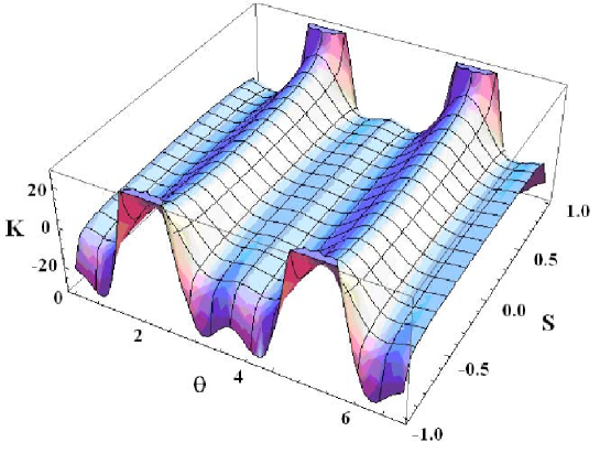
Figure 1: Color online. The parameter $K(\theta,S)$ signifying chaotic behavior plotted according to Eq. (18) for the following values of the parameters $\beta=3$,$\varepsilon=0.5$.

Equation (19) defiance the width of the chaotic domain where parameter of chaos (18) is larger than one $K>1$. Obviously, the width of the chaotic domain depends on the values of anisotropy and easy to see that in case of small anisotropy area of chaos is narrower than in zero anisotropy case $\Delta\theta(\varepsilon=0)>\Delta\theta(\varepsilon<<1)$. Therefore we conclude that small anisotropy leads to the less chaotic regime.

From the parameter of the chaos (18) (also plotted in Fig. 1) we conclude that the phase space of the system consists of domains corresponding to a regular and a chaotic motion. Later we will use the random phase approximation, which is valid precisely in the latter domain.Zaslavsky

In order to obtain explicit expressions for the spin correlation functions we rewrite the recurrence relations in Eqs. (II) in the following form

$$\theta_{n+1}=\theta_{n}+\omega(s_{n+1})=\theta_{n}+\omega_{\nu}\big{(}S_{n}-\beta V^{\prime}(\theta)\big{)}=$$

$$=\theta_{n}+\omega_{\nu}(S_{n})-\beta V^{\prime}(\theta)\omega^{\prime}_{\nu}(S_{n})=$$ (21)

$$=\theta_{n}+\omega_{\nu}(S_{n})-\beta\bigg{(}\sin 2\theta_{n}-\frac{\varepsilon}{2}\sin 4\theta_{n}\bigg{)}\,.$$

For the angular variable we infer the self-consistent recurrence relation

$$\theta_{n+1}=\theta_{n}+\omega_{\nu}(S_{n})-\beta\bigg{(}\sin 2\theta_{n}-\frac{\varepsilon}{2}\sin 4\theta_{n}\bigg{)}.$$ (22)

The correlation function is given by

$$\langle S_{n+1}|S_{j}\rangle = \frac{1}{2\pi}\int\limits_{0}^{2\pi}d\theta_{0}e^{i(\theta_{n}-\theta_{0})}=$$ (23)

$$= \frac{1}{2\pi}\int\limits_{0}^{2\pi}d\theta_{0}e^{i\bigg{(}\theta_{n-1}+\omega_{\nu}(S_{n-1})-K_{0}\sin 2\theta_{n-1}+\frac{K_{0}\varepsilon}{2}\sin 4\theta_{n-1}-\theta_{0}\bigg{)}}$$

and can be calculated using the above iterative procedure as well as the expression for the Bessel function $\exp(iz\sin\varphi)=\sum\limits_{m=-\infty}^{+\infty}J_{m}(z)e^{im\varphi}$. Taking into account that $\omega_{\nu}(S_{n})=\omega\approx const$, $K_{0}=\beta\omega^{\prime}(S_{n})\approx const$, from Eq. (23) we deduce

$$\langle S_{j+n}|S_{j}\rangle=\frac{1}{2\pi}\int\limits_{0}^{2\pi}d\theta_{0}e^{i(\theta_{n}-\theta_{0})}=$$

$$=\frac{1}{2\pi}\int\limits_{0}^{2\pi}d\theta_{0}e^{i(\theta_{n-1}-\theta_{0})}\cdot e^{-iK_{0}\sin 2\theta_{n-1}}\cdot e^{\frac{iK_{0}\varepsilon}{2}\sin 4\theta_{n-1}}=$$

$$=\frac{1}{2\pi}\int\limits_{0}^{2\pi}d\theta_{0}e^{i(\theta_{n-1}-\theta_{0})}\cdot\sum\limits_{m_{1}=-\infty}^{+\infty}J_{m_{1}}(K_{0})e^{-2im_{1}\theta_{n-1}}\cdot\sum\limits_{l_{1}=-\infty}^{+\infty}J_{l_{1}}\bigg{(}\frac{K_{0}\varepsilon}{2}\bigg{)}e^{4il_{1}\theta_{n-1}}=$$ (24)

$$=e^{in\omega}\sum\limits_{m_{1}=-\infty}^{+\infty}\sum\limits_{m_{2}=-\infty}^{+\infty}\ldots\sum\limits_{m_{n}=-\infty}^{+\infty}\sum\limits_{l_{1}=-\infty}^{+\infty}\sum\limits_{l_{2}=-\infty}^{+\infty}\ldots\sum\limits_{l_{n}=-\infty}^{+\infty}(-1)^{l_{1}+l_{2}+\ldots+l_{n}}\cdot$$

$$\cdot e^{-2i\omega m_{1}}e^{-2i\omega(m_{1}+m_{2})}\ldots e^{-2i\omega(m_{1}+m_{2}+\ldots+m_{n-1})}e^{-2i\omega l_{1}}e^{-2i\omega(l_{1}+l_{2})}\ldots e^{-2i\omega(l_{1}+l_{2}+\ldots+l_{n-1})}\cdot$$

$$\cdot J_{m_{1}}[K_{0}]J_{m_{2}}[(1-2m_{1}+4l_{1})K_{0}]\ldots J_{m_{n}}[(1-2(m_{1}+m_{2}\ldots+m_{n-1})+4(l_{1}+l_{2}\ldots+l_{n-1}))K_{0}]\cdot$$

$$\cdot J_{l_{1}}\bigg{[}\frac{K_{0}\varepsilon}{2}\bigg{]}\ldots J_{l_{n}}\bigg{[}\frac{1-2(m_{1}+m_{2}\ldots+m_{n-1})+4(l_{1}+l_{2}\ldots+l_{n-1}))K_{0}\varepsilon}{2}\bigg{]}\cdot$$

$$\cdot\delta_{1-2(m_{1}+m_{2}+\ldots+m_{n})+4(l_{1}+l_{2}+\ldots+l_{n});1}\,.$$

For the details of the derivation of Eq.(24) see Appendix C.

In the case of a large Lyapunov exponent $J_{m}(K_{0})\sim(K_{0})^{-1/2}$, $K_{0}\gg 1$ we infer from (III)

$$\langle S_{j+n}|S_{j}\rangle\sim\frac{e^{in\omega}}{(K_{0}^{2}\varepsilon/2)^{n/2}}=\exp\bigg{(}-\frac{n}{\tau_{c}}\bigg{)}e^{in\omega}\,,$$ (25)

where $\tau_{c}=2/\ln\bigg{(}\frac{K_{0}^{2}\varepsilon}{2}\bigg{)}$ is the correlation length. Since $K_{0}\sim\beta$, we have the following estimation

$$\tau_{c}\sim\frac{2}{\ln\bigg{(}\frac{\beta^{2}\varepsilon}{2}\bigg{)}}\,.$$ (26)

In the isotropic case $\varepsilon=0$, one can perform the same calculations [insertion of $\varepsilon=0$ into Eq. (26) gives a wrong result] and show that

$$\tau^{\prime}_{c}\sim\frac{2}{\ln\beta}\,$$ (27)

holds. Taking into account Eqs. (26), (27) and expressions for the rescaled interaction constants $\varepsilon\rightarrow\frac{J-g}{2g},~{}~{}\beta\rightarrow\frac{\beta}{g}$ we conclude that the role of the anisotropy is not trivial. Namely, the strong anisotropy

$$J-g>\frac{4g^{2}}{\beta},$$ (28)

suppresses the spin correlations because then $\tau^{\prime}_{c}>\tau_{c}$. On the other hand the weak anisotropy

$$J-g<\frac{4g^{2}}{\beta},$$ (29)

enhances the correlations $\tau^{\prime}_{c}<\tau_{c}$.

It should be stressed that the reliability of the analytical estimates is limited. This is particularly apparent for the case where the numerical and the analytical predictions deviate from each others, due to limited range of applicability of the analytical expressions, derived after rough approximations.

The role of the anisotropy $\varepsilon=(J-g)/2g$ can be clarified numerically as well. In order to better understand the physical features of the model (1) we will study the phase portrait of the system. The results of the numerical evaluation of the recurrence relations (II) are presented in Figs. 2-5.

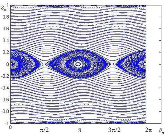
Figure 2: Color online. Results of the numerical calculations of the recurrence relations (II) on the phase plane $(S_{n},\theta_{n})$. The following the parameters are used $\beta=0.05$, $\varepsilon=0.005$. About hundred trajectories are generated for the set of different initial conditions $(S_{0},\theta_{0})$.

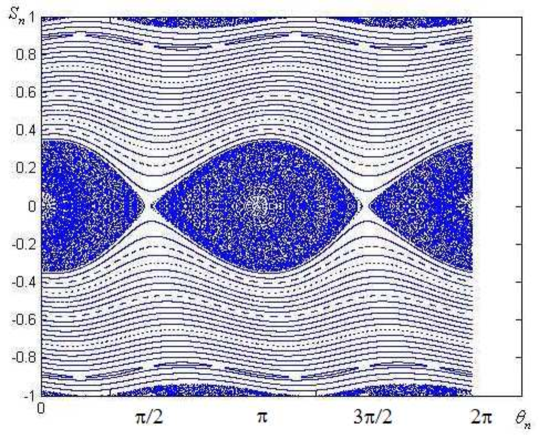
Figure 3: Color online. Results of the numerical calculations of the recurrence relations (II) on the phase plane $(S_{n},\theta_{n})$, for following the parameters: $\beta=0.05$, $\varepsilon=0$. About hundred trajectories are generated for the set of different initial conditions $(S_{0},\theta_{0})$.

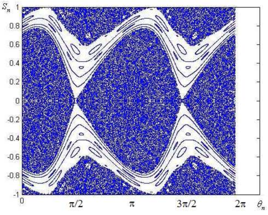
Figure 4: Color online. Results of the numerical calculations of the recurrence relations (II) on the phase plane $(S_{n},\theta_{n})$. We used $\beta=0.3$, $\varepsilon=0.15$. About hundred trajectories are generated for the set of different initial conditions $(S_{0},\theta_{0})$.

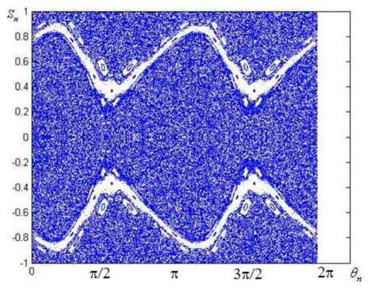
Figure 5: Color online. Results of the numerical calculations of the recurrence relations (II) on the phase plane $(S_{n},\theta_{n})$, for the following parameters: $\beta=0.3$, $\varepsilon=0$. About hundred trajectories are generated for the set of different initial conditions $(S_{0},\theta_{0})$. With the increase of the value of parameter $\beta$, the domain of the chaotic motion covers almost the whole phase space (See Fig. 4, Fig.5), because the chaos parameter $K$ Eq.(18) is proportional to the constant $\beta$.

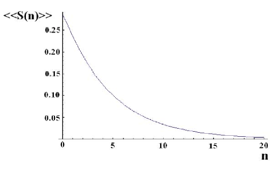
Figure 6: Results of the numerical integration for the statistically averaged random alignment factor $\ll\sin^{2}(\theta_{n}-\theta_{n-1})\gg$ in the diffusive approximation (IV), for $\beta=0.3$ and $\varepsilon=0.15$.

As we see from Fig. 2 the phase space of the system consists of two topologically different domains separated from each other by a separatrix. Most of the phase space belongs to the domain of the regular motion and open phase trajectories. The domain of closed phase trajectories mainly corresponds to the irregular motion and a small island of a regular motion is observed only in the center of the portrait. From this formal mathematical statement, one can extract interesting physical information. Closed trajectories belong to the oscillatory regime and open trajectories to the rotational one. Therefore, we expect that two types of motion can be realized for the model (1). The domain of the regular spin rotational motion is defined by the relation $0.2<|S_{n}|<1$. If then $|S_{n}|<0.2$ the spin oscillation is chaotic and only for very small amplitude an island of regular oscillations is observed in the center. If the anisotropy parameter is zero $\varepsilon=0$ then the island of the regular oscillatory motion disappears (see Fig. 3). This means that without the small anisotropy the spin system is less correlated [see Eqs. (28) and (29)]. Such a geometrical interpretation can be extrapolated from the pair of the canonical variables $(S_{n},\theta_{n})$ to the real spin variables $S_{n}^{z}=\cos\theta_{n}$ using the parametrization (2) and a simple relation $S_{n}=\sin(\theta_{n}-\theta_{n-1})$.

IV Spin diffusion and kinetic approach

The dynamical picture does not apply in the chaotic regime for $K>0$ or $K<-4$. An adequate language in this case is the statistical approach. Instead of the dynamical variables the key role is played by the probability distribution function, which is a solution of the Fokker-Planck equation. Its derivation is rather straightforward for chaotic dynamical models and is based on the Kolmogorov, Arnold, Moser (KAM) theory.Berakdar Interested reader can find all technical details of the derivation for the spin chain model in the recent work Iomin . Here we are using the final result adopted to the SMM system. The probability distribution of the spin variable $S_{n}=\sin(\theta_{n}-\theta_{n-1})$ is described by following diffusion equation:

$$\frac{\partial f}{\partial t}=D\frac{\partial^{2}f}{\partial S^{2}}\,,$$ (30)

where $D(S)=\frac{\beta^{2}}{4}\bigg{(}1+\frac{\varepsilon^{2}}{4}\bigg{)}$ is the diffusion coefficient. For the details of derivation of Eq.(30) see Appendix B. The fundamental solution of this equation is

$$f(S,t)=\frac{1}{2\sqrt{\pi Dt}}\exp\bigg{(}-\frac{S^{2}}{4Dt}\bigg{)},$$ (31)

and can be found in many classical textbooks (see e. g. Tikhonov ). This solution (31) is defined on the interval $-\infty<S<\infty$ whereas we need one for $-1\leq S\leq 1$. In order to find a solution relevant to our problem we will consider the following boundary and initial conditions for the diffusion equation (30).

$$f=W_{0}~{}~{}~{}~{}~{}\mbox{for}~{}~{}~{}~{}~{}t=0,$$

$$f=g_{1}(t)~{}~{}~{}~{}~{}\mbox{for}~{}~{}~{}~{}~{}S=-1,$$ (32)

$$f=g_{2}(t)~{}~{}~{}~{}~{}\mbox{for}~{}~{}~{}~{}~{}S=1,$$

and will look for the solution in the following form

$$f(S,t)=2\sum\limits_{m=1}^{\infty}\sin(m\pi S)\exp\big{(}-Dm^{2}\pi^{2}t\big{)}M_{m}(t),$$ (33)

where

$$M_{m}(t)=\int\limits_{0}^{1}f_{0}(\xi)\sin(n\pi\xi)d\xi+Dm\pi\int\limits_{0}^{1}\exp\big{(}Dm^{2}\pi^{2}\tau\big{)}\big{[}g_{1}(\tau)-(-1)^{m}g_{2}(\tau)\big{]}d\tau.$$ (34)

In the simple case $g_{1}(t)=g_{2}(t)=0$ we obtain from Eqs. (30)-(34)

$$f(S,t)=\frac{4W_{0}}{\pi}\sum\limits_{m=0}^{\infty}\frac{1}{(2m+1)}\sin\big{(}(2m+1)\pi S\big{)}\exp\big{(}-D(2m+1)\pi^{2}t\big{)},$$ (35)

where the coefficient $W_{0}$ can be defined from the normalization condition $\int\limits_{-1}^{+1}\int\limits_{0}^{+\infty}f(S,t)dSdt=1$, $W_{0}=\frac{D\pi^{4}}{7\varsigma(3)}$. Here $\varsigma(s)=\sum\limits_{k=1}^{\infty}k^{-s}$ is the Riemann zeta function Abramowitz . We note the direct correspondence between the fictitious time and the spin index $t\rightarrow nT$, $T=1$ Eq. (II). For the averages of the discrete random variable $S\equiv S_{n}=\sin(\theta_{n}-\theta_{n-1})$ we follow the standard procedure (see Chotorlishvili , Eq.(18)-(20)) and utilize the distribution function Eq. (35). The integration is performed over the interval $-1\leqslant S_{n}\leqslant 1$. As a result we obtain:

$$\ll S^{2}_{n}\gg=\ll S^{2}\gg=\ll\sin^{2}(\theta_{n}-\theta_{n-1})\gg=\int\limits_{-1}^{+1}S^{2}f(S,t)dS=$$

$$=\frac{4W_{0}}{\pi}\sum\limits_{m=0}^{\infty}\frac{1}{(2m+1)}\int\limits_{-1}^{+1}S^{2}\sin\big{(}(2m+1)\pi|S|\big{)}dS\cdot\exp\big{(}-D(2m+1)\pi^{2}t\big{)}.$$ (36)

After an integration we get:

$$\ll S^{2}\gg=\ll\sin^{2}(\theta_{n}-\theta_{n-1})\gg=$$

$$=\frac{4W_{0}}{\pi^{2}}e^{-D\pi^{2}n}F\bigg{(}\bigg{\{}\frac{1}{2},\frac{1}{2},1\bigg{\}},\bigg{\{}\frac{3}{2},\frac{3}{2}\bigg{\}},e^{-2D\pi^{2}n}\bigg{)}-\frac{W_{0}}{\pi^{4}}e^{-D\pi^{2}n}\Phi\bigg{(}e^{-2D\pi^{2}n},4,\frac{1}{2}\bigg{)}\,,$$ (37)

where $F(\{a_{1}\ldots a_{p}\};\{b_{1}\ldots b_{q}\};z)=\sum\limits_{k=0}^{\infty}\frac{(a_{1})_{k}\ldots(a_{p})_{k}}{(b_{1})_{k}\ldots(b_{q})_{k}}\cdot\frac{z^{k}}{k!}$ is the generalized hypergeometric function and $\Phi(z,s,a)=\sum\limits_{k=0}^{\infty}\frac{z^{k}}{(k+a)^{s}}$ is the generalized Riemann zeta function. Abramowitz From Eq. (IV) we immediately see that the statistically averaged random alignment factor $\ll\sin^{2}(\theta_{n}-\theta_{n-1})\gg$ is not uniform along the spin chain (see Fig. 6), but rather decays exponentially with $n$. This result is reasonable since the solution for the distribution function (35) is obtained via deterministic initial and boundary conditions (IV). Therefore, a maximum of correlation is expected for $n=0$. Since $t=nT$, $t=0$, $n=0$ corresponds to the boundary where the distribution function is defined precisely. Far away from the boundary that means for $n>>1$ randomness occurs and the correlation decays.

V Conclusions

In this paper we considered an anisotropic nonlinear spin chain, which serves as a model for a chain of coupled nanomagnets. We have shown, that there is a direct map between an infinite-dimensional spin chain model and an equivalent effective $1D$ classical Hamiltonian with a discrete fictitious time-dependent perturbation. We have established a direct connection between the dynamical characteristics of the classical system and the spin correlation time of the original quantum chain. The decay rate for the spin correlation functions turns out to depend logarithmically on the maximal Lyapunov exponent. In addition, for an anisotropic couplings we found an interesting counterintuitive feature: the small anisotropy leads to the formation of small islands of the regular motion in a chaotic sea of the system’s phase space. As a result, the spin correlations become stronger within the islands of regular motion. We argue that these results obtained within the classical approximation are interesting in other regimes. If the Lyapunov regime is reached for a quantum system, which takes place for the Lyapunov exponent $\lambda<J^{2}/\Delta$, where $\Delta$ is the mean level spacing and $J$ is the exchange interaction constant between spins, then the decay rate for the teleportation fidelity in a device based on such spin chains is directly related to $\lambda$.

Acknowledgments: We thank Boris Fine for useful discussions. The financial support by the Deutsche Forschungsgemeinschaft (DFG) through SFB 762, contract BE 2161/5-1, the Grant No. KO-2235/3, and STCU Grant No. 5053 is gratefully acknowledged.

Appendix A Derivation of the recurrence relations

Let us consider the equilibrium state for the model (3):

$$\frac{\partial H}{\partial\varphi_{n}}=\bigg{(}\cos(\theta_{n}-\theta_{n+1})-\cos(\theta_{n}+\theta_{n+1})\bigg{)}\sin(\varphi_{n+1}-\varphi_{n})-$$

$$-\bigg{(}\cos(\theta_{n-1}-\theta_{n})-\cos(\theta_{n-1}+\theta_{n})\bigg{)}\sin(\varphi_{n+1}-\varphi_{n}),$$ (38)

$$\frac{\partial H}{\partial\theta_{n}}=-\frac{J}{2}\bigg{(}\sin(\theta_{n}+\theta_{n+1})+\sin(\theta_{n-1}+\theta_{n})+\sin(\theta_{n}-\theta_{n+1})-\sin(\theta_{n-1}+\theta_{n})-$$

$$-\frac{g}{2}\bigg{(}\sin(\theta_{n}-\theta_{n+1})-\sin(\theta_{n-1}-\theta_{n})-\sin(\theta_{n}+\theta_{n+1})-\sin(\theta_{n-1}+\theta_{n})\bigg{)}\cos(\varphi_{n+1}-\varphi_{n})+$$

$$+\beta\sin 2\theta_{n}=0.$$ (39)

After introduction of the notation $S_{n}=\sin(\theta_{n}-\theta_{n-1})$, from (38), (39) we find:

$$\Bigg{(}\frac{J}{2}+\frac{g}{2}\Bigg{)}S_{n+1}-\Bigg{(}\frac{J}{2}+\frac{g}{2}\Bigg{)}S_{n}-\Bigg{(}\frac{J}{2}-\frac{g}{2}\Bigg{)}\sin(\theta_{n}+\theta_{n+1})-$$

$$-\Bigg{(}\frac{J}{2}-\frac{g}{2}\Bigg{)}\sin(\theta_{n-1}+\theta_{n})+\beta\sin(2\theta_{n})=0,$$ (40)

$$\varphi_{n+1}=\varphi_{n}+\pi m,~{}~{}~{}m=0,1\,.$$

Let the asymmetry parameter be defined by $\varepsilon=|J-g|$, $\varepsilon<J,g$. Next we perform a rescaling of the interaction constants $\frac{\varepsilon}{2g}\rightarrow\varepsilon$, $\beta\rightarrow\mp\frac{\beta}{g}$. From (A) we deduce:

$$(S_{n+1}-S_{n})-\varepsilon\sin(\theta_{n}+\theta_{n+1})\varepsilon-\sin(\theta_{n-1}+\theta_{n})+\beta\sin(2\theta_{n})=0,$$ (41)

$$\theta_{n+1}=\theta_{n}+\pi\nu+(-1)^{\nu}\arcsin[S_{n+1}],~{}~{}~{}\nu=0,1\,.$$

Depending on the sign of the rescaled barrier height $\beta\rightarrow\mp\frac{\beta}{g}$, the value of the index $m=0,1$ defines the energy minimum condition. For convenience we will use positively defined $\beta>0$ and consequently $m=0$. In the simplest case $\nu=0$, so that from (41) we obtain:

$$(S_{n+1}-S_{n})$$

$$-\varepsilon\Bigg{(}\sin[2\theta_{n}]\sqrt{1-S_{n+1}^{2}}+\cos(2\theta_{n})S_{n+1}+\sin(2\theta_{n})\sqrt{1-S_{n}^{2}}-\cos(2\theta_{n})S_{n+1}\Bigg{)}+$$ (42)

$$+\beta\sin(2\theta_{n})=0\,.$$

Retaining only the first order terms with respect to the small parameter $\varepsilon=\frac{|J-g|}{2g}$, from (A) we obtain the following recurrence relations (II):

$$S_{n+1}=S_{n}-\beta\bigg{(}\sin 2\theta_{n}-\frac{\varepsilon}{2}\sin 4\theta_{n}\bigg{)},$$

$$\theta_{n+1}=\theta_{n}+\omega_{\nu}(S_{n+1}),$$ (43)

$$\omega_{\nu}(S_{n})=\pi\nu+(-1)^{\nu}\arcsin S_{n}\,.$$

Appendix B Derivation of the kinetic equation

The starting point for the derivation of the kinetic equation is the equivalent effective Hamiltonian (II):

$$\frac{dS}{dt}=-\frac{\partial H}{\partial\theta}=-\beta V^{\prime}(\theta)T\sum\limits_{n=-\infty}^{+\infty}\delta(t-nT),$$

$$\frac{d\theta}{dt}=\frac{\partial H}{\partial S}=\omega(S),$$ (44)

$$\omega_{\nu}(S)=\pi\nu+(-1)^{\nu}\arcsin s\,.$$

Here the variable $S$ plays the role of the adiabatic (slowly varying) action variable, while the angular variable $\theta$ is the fast variable. Due to the presence of the two different time scales in the system:

$$H=H_{0}(S)+\varepsilon V(S,\theta,t)$$ (45)

for the derivation of the kinetic equation we will follow to the standard procedure. Toklikishvili The distribution function of the random variable $f(S,t)$ obeys the Liouvillian equation of motion:

$$i\frac{\partial f_{0}}{\partial t}=(\hat{L}_{0}+\varepsilon\hat{L}_{1})f_{0},$$

$$\hat{L}_{0}=i\omega(S)\frac{\partial}{\partial\theta},$$ (46)

$$\hat{L}_{1}=-i\Bigg{(}\frac{\partial V}{\partial S}\frac{\partial}{\partial\theta}-\frac{\partial V}{\partial S}\frac{\partial}{\partial\theta}\Bigg{)}.$$

The formal solution of the Liouville equation with the accuracy of second order terms in the small parameter $\varepsilon$ reads:

$$f_{0}(S,t)=f(S,0)-i\varepsilon\sum\limits_{m}\int\limits_{0}^{t}dt_{1}\exp[im\int\limits_{0}^{t_{1}}\omega(t^{\prime})dt^{\prime}]\langle n|\hat{L}_{1}|m\rangle f_{0}(S,0)+$$

$$+(-i\varepsilon)^{2}\sum_{m}\int\limits_{0}^{t}dt_{1}\int\limits_{0}^{t_{1}}dt_{2}\exp[-im\int\limits_{t_{1}}^{t_{2}}\omega(t^{\prime})dt^{\prime}]\langle 0|\hat{L}_{1}(t_{1})|m\rangle\langle m|\hat{L}_{1}(t_{2})|0\rangle f_{0}(S,0).$$ (47)

Here $\langle n|\hat{L}_{1}|m\rangle\frac{1}{2\pi}\int\limits_{0}^{2\pi}d\theta e^{-in\theta}\hat{L}_{1}e^{im\theta}$ is the matrix element of the Liouville operator. After averaging over the initial phases $f(I,t)=\ll f_{0}(I,t)\gg$ and applying the random phase approximation with respect to the fast chaotic variable $\Psi(t_{2},t_{1})=\int\limits_{t_{1}}^{t_{2}}\omega(t^{\prime})dt^{\prime}=\theta(t_{1})-\theta(t_{2})$

$$\ll\exp im\Psi(t_{2},t_{1})\gg\approx\exp(-(t_{1}-t_{2})/\tau_{c})\exp(-im\omega(t_{1}-t_{2}))\,.$$ (48)

From (B) we obtain:

$$\frac{\partial f}{\partial t}=-2\varepsilon^{2}\sum\limits_{m>0}\sum\limits_{p>0}\frac{(1/\tau_{c})\langle 0|\hat{L}_{1p}|m\rangle\langle m|\hat{L}_{1-p}|0\rangle f}{(1/\tau_{c})^{2}+(m\omega-p\Omega)^{2}}\,,$$ (49)

where

$$\langle 0|\hat{L}_{1p}|m\rangle\langle m|\hat{L}_{1-p}|0\rangle=$$

$$=\bigg{(}\frac{\Omega}{2\pi}\bigg{)}^{2}\frac{1}{(2\pi)^{2}}\int\limits_{-T/2}^{T/2}dt_{1}\int\limits_{-T/2}^{T/2}dt_{2}\int\limits_{0}^{2\pi}d\theta^{\prime}\int\limits d\theta"\hat{L}_{1}(t_{1})e^{im(\theta^{\prime}-\theta")}\hat{L}_{1}(t_{2})e^{-ip\Omega(t_{1}-t_{2})}$$ (50)

and the following notation is used $\tau_{c}=2T/\ln K$, $T=\frac{2\pi}{\Omega}$. After calculating the integrals in (B), in the limit $\frac{1}{\tau_{c\Omega}}\rightarrow 0$, $T=1$ form (49) we simply recover the diffusion equation (30):

$$\frac{\partial f(S,t)}{\partial t}=\frac{\partial}{\partial S}D(S)\frac{\partial f(S,t)}{\partial S},$$ (51)

$$D(S)=\frac{\beta^{2}}{4}\Bigg{(}1+\frac{\varepsilon^{2}}{4}\Bigg{)}\,.$$ (52)

More details of derivations can be found in Ref. Toklikishvili,

Appendix C Correlation functions

For the evaluation of the multiple series in Eq. (III) one should sum up the contributions from the main non-oscillatory terms. Due to the delta function $\delta_{1-2(m_{1}+m_{2}+\ldots+m_{n})+4(l_{1}+l_{2}+\ldots+l_{n}),1}$ in Eq. (III), and the fast exponential factors $e^{i4\omega(l_{1}+l_{2}+\ldots+l_{n})}$, $e^{-2i\omega(m_{1}+m_{2}+\ldots+m_{n})}$, the relevant terms in Eq. (III) are those with

$$m_{1}+m_{2}+\ldots+m_{n}=0,$$

$$l_{1}+l_{2}+\ldots+l_{n}=0.$$ (53)

Using the asymptotic expressions for Bessel functions:

$$J_{m}(K_{0})\sim K_{0}^{-1/2},~{}~{}\mbox{for}~{}~{}K_{0}\gg 1,$$ (54)

and condition (C), one can easily obtain (26) from (III).

References

- (1) D. Bruss and G. Leuchs, Lectures on Quantum Information, Wiley VCH Verlag Weinheim (2007).
- (2) J. Raimond, M. Brune, S. Haroche, Rev. Mod. Phys. 73, 565 (2001), V. Vedral and E. Kashe, Phys. Rev. Lett. 89, 037903 (2002).
- (3) L. Amico, R. Fazio, A. Osterloh, V. Vedral, Rev. Mod. Phys. 80, 517 (2008).
- (4) H. Mabuchi, A. Doherty, Science 298, 1372 (2002).
- (5) J.Q. You, F. Nori Physics Today 58, 42 (2005); S.N. Shevchenko, S. Ashhab, F. Nori, Phys. Rep. 492, 1 (2010); Y. Makhlin, G. Schön, A. Shnirman, Rev. Mod. Phys. 73, 357 (2001).
- (6) M. Harlander, M. Brownnutt, W. Hänsel, R. Blatt, New J. Phys. 12, 093035 (2010); F. Zähringer, G. Kirchmair, R. Gerritsma, E. Solano, R. Blatt, C. F. Roos, Phys. Rev. Lett. 104, 100503 (2010).
- (7) R. Sessoli, D. Gatteschi, A. Caneschi, and M. A. Novak, Nature 365, 141 (1993).
- (8) Gunther L and Barbara B (ed) Quantum Tunneling of Magnetization, (Dordrech: Kluwer-Academic) (1995).
- (9) J. R. Friedman, M. P. Sarachik , J. Tejada, and R. Ziolo, Phys. Rev. Lett. 76, 3830 (1996), E. M. Chudnovsky and D. A. Garanin, Phys. Rev. B 81, 214423 (2010), D. A. Garanin and E. M. Chudnovsky, Phys. Rev. Lett. 102, 097206 (2009).
- (10) J. M. Hernandez, X. X. Zhang, F. Luis, J. Bartolome, J. Tejada and R. Ziolo Europhys. Lett. 35, 301 (1996).
- (11) L. Thomas, F. Lionti, R. Ballou, D. Gatteschi, R. Sessoli and B. Barbara Nature 383, 145 (1996).
- (12) E. M. Chudnovsky and J. Tajida, Macroscopic Quantum Tunneling of the Magnetic Moment (Cambrige: Cambridge University Press) (1998).
- (13) L. Thomas, F. Lionti, R. Ballou, D. Gatteschi, R. Sessoli, and B. Barbara, Nature 383, 145 (1996).
- (14) W. Wernsdorfer and R. Sessoli, Science 284, 133 (1999).
- (15) M. Hennion et al., Phys. Rev. B 56, 8819 (1997).
- (16) W.Wernsdorfer, N. Aliaga-Alcalde, D. N. Hendrickson, and G. Christou, Nature 416, 406 (2002).
- (17) R. Tiron, W. Wernsdorfer1, D. Foguet-Albiol, N. Aliaga-Alcalde, and G. Christou, Phys. Rev. Lett. 91, 227203 (2003).
- (18) A. Ardavan, O. Rival, J. J. L. Morton, S. J. Blundell, A. M. Tyryshkin, G.A. Timco, and R. E. P. Winpenny, Phys. Rev. Lett. 98, 057201(2007), D. A. Garanin and E. M. Chudnovsky Phys. Rev. B 59, 3671 (1999), O. Waldmann, Phys. Rev. B 75, 174440 (2007).
- (19) A. Candini, G. Lorusso, F. Troiani, A. Ghirri, S. Carretta,3, P. Santini, G. Amoretti, C. Muryn, F. Tuna, G. Timco, E. J. L. McInnes, R. E. P. Winpenny, W. Wernsdorfer, and M. Affronte, Phys. Rev. Lett. 104, 037203 (2010).
- (20) W. Wernsdorfer, T. C. Stamatatos, and G. Christou, Phys. Rev. Lett. 101, 237204 (2008).
- (21) R. Tiron, W.Wernsdorfer, D. Foguet-Albiol, N. Aliaga-Alcalde, and G. Christou, Phys. Rev. Lett. 91, 227203 (2003).
- (22) L. Chotorlishvili, Z. Toklikishvili, P. Schwab, and J. Berakdar, Phys. Rev. B 82, 014418 (2010).
- (23) L. Chotorlishvili, P. Schwab, J. Berakdar, J. Phys. Cond. Mat. 22, 036002 (2010).
- (24) L. Chotorlishvili, P. Schwab, Z. Toklikishvili, J. Berakdar J. Comp.Theor. Nanoscience 7, 2430, (2010).
- (25) A. Iomin Phys. Rev. E 70, 026206 (2004).
- (26) Ph. Jacquod, P.G. Silvestrov, and C.W.J. Beenakker Pys. Rev. E 64, 055203 (2001).
- (27) G. M. Zaslavsky, The Physics of Chaos in Hamiltonian Systems 2nd edn (London: Imperial College) (2007).
- (28) M. Abramowitz and I. Stegun (ed), Handbook of Mathematical Functions (Applied Mathematics Series vol. 55) (Washington: National Bureau of Standards) (1972).
- (29) L. Chotorlishvili, Z. Toklikishvili, J. Berakdar, J. Phys. Cond. Mat., 21, 356001 (2009).
- (30) A. N. Tikhonov A. A. Samarsky, Equations of Mathematical Physics, (in Russian), ”Nauka” Moscow (1966).