Uncovering missing links with cold ends

Abstract

To evaluate the performance of prediction of missing links, the known data are randomly divided into two parts, the training set and the probe set. We argue that this straightforward and standard method may lead to terrible bias, since in real biological and information networks, missing links are more likely to be links connecting low-degree nodes. We therefore study how to uncover missing links with low-degree nodes, namely links in the probe set are of lower degree products than a random sampling. Experimental analysis on ten local similarity indices and four disparate real networks reveals a surprising result that the Leicht-Holme-Newman index [E. A. Leicht, P. Holme, and M. E. J. Newman, Phys. Rev. E 73, 026120 (2006)] performs the best, although it was known to be one of the worst indices if the probe set is a random sampling of all links. We further propose an parameter-dependent index, which considerably improves the prediction accuracy. Finally, we show the relevance of the proposed index on three real sampling methods.

1 Introduction

Many social, biological, and information systems can be well described by networks, where nodes represent individuals and links denote the relations or interactions between nodes. The study of complex networks has therefore become a common focus of many branches of science. A fundamental tool for network analysis is the so-called link prediction, which attempts to estimate the likelihood of the existence of a link between two nodes, based on observed links and the attributes of nodes [1, 2].

In many biological networks, such as food webs, protein-protein interaction networks and metabolic networks, whether a link between two nodes exists must be demonstrated by field and/or laboratory experiments, which are usually very costly. Our knowledge of these networks is very limited, for example, 80% of the molecular interactions in cells of Yeast [3] and 99.7% of human [4, 5] are still unknown. Instead of blindly checking all possible interactions, to predict based on known interactions and focus on those links most likely to exist can sharply reduce the experimental costs if the predictions are accurate enough. Social network analysis also comes up against the missing data problem [6, 7], where link prediction algorithms may play a role. In addition, the data in constructing biological and social networks may contain inaccurate information, resulting in spurious links [8, 9]. Link prediction algorithms can be applied to identify these spurious links [10]. Besides helping in analyzing networks with missing data, the link prediction algorithms can be used to predict the links that may appear in the future of evolving networks. For example, in online social networks, very likely but not yet existent links can be recommended as promising friendships, which can help users in finding new friends and thus enhance their loyalties to the web sites. Other applications of link prediction include the evaluation of network evolving models [11], the classification of partially labeled networks [12], and so on (see the review article [1] for the detailed discussion on real applications).

To evaluate the algorithmic performance, the data set is divided into two parts: the training set is treated as known information while the probe set is used to estimate the prediction accuracy. To our knowledge, the datasets are always divided completely randomly. This is of course the most straightforward way, and it seems a very fair method without any statistical bias. However, this straightforward and standard method may lead to terrible bias, since in real biological and information networks, missing links are more likely to be links connecting low-degree nodes. For example, the known structure of the World Wide Web is just a sampling, where the hyperlinks from popular web pages have higher probability to be uncovered. In contrast, hyperlinks from unbeknown web pages are probably lost. Actually, in common sense, interaction between two significant proteins, hyperlink between two well-known web pages and relationship between two famous persons are of less probability to be missed. Accordingly, in this article, we study how to uncover missing links with low-degree nodes. That is to say, we divide the data set into two parts and make the links in the probe set less popular (i.e., of less degree products) than the links in the training set. Experimental analysis on ten local similarity indices and four disparate real networks reveals a surprising result that the Leicht-Holme-Newman (LHN) index [13] performs the best, although it was known to be one of the worst indices if the probe set is a random sampling of all links [14]. We further propose an parameter-dependent index, which considerably improves the prediction accuracy. Finally, we show the relevance of the proposed index on three real sampling methods.

This article is organized as follows. In the next section, we will clearly define the problem of link prediction, describe the standard process to evaluate the prediction accuracy, introduce the state-of-the-art local indices for node similarity and how to sample less popular links for the probe set. Experimental results for the traditional sampling method and the proposed method are presented in Section III. In Section IV, we will propose an improved index which performs even better than the LHN index. In Section V, we will introduce three mainstream sampling methods, and test the improved index on the corresponding sampled networks. Finally, we summarize our results in Section VI.

2 Problem Description

2.1 Link Prediction: Problem and Evaluation

Given an undirected network $G(V,E)$, where $V$ and $E$ are the sets of nodes and links respectively. The multiple links and self-connections are not allowed. Denote by $U$ the universal set containing all $\frac{|V|(|V|-1)}{2}$ possible links, where $|V|$ denotes the number of elements in set $V$. Then, the set of nonexistent links is $U\backslash E$, in which there are some missing links, namely the existed yet unknown links or those that will form in the future. The task of link prediction is to uncover these links. Each node pair $x$ and $y$ will be assigned a score $s_{xy}$ according to a given prediction algorithm. The higher score, the higher probability that this link exists. The score matrix $S$ is symmetry for $G$ is undirected. All the nonexistent links are sorted in descending order according to their scores, and the top-ranked links are most likely to exist.

To test the algorithmic accuracy, the observed links $E$ are divided into two groups: the training set $E^{T}$ is treated as known information, while the probe set $E^{P}$ is used for testing and no information therein is allowed to be used for prediction. Clearly, $E=E^{T}\cup E^{P}$ and $E^{T}\cap E^{P}=\phi$. The accuracy of prediction is quantified by a standard metric called AUC (short for area under the receiver operating characteristic curve) [15]. Specifically, this metric can be interpreted as the probability that a randomly chosen missing link (links in $E^{P}$) has higher score than a randomly chosen nonexistent link (links in $U\backslash E$). In the implementation, among $n$ times of independent comparisons, if there are $n^{\prime}$ times that the missing link has higher score and $n^{\prime\prime}$ times the missing link and nonexistent link have the same score, AUC is calculated by $\frac{n^{\prime}+0.5n^{\prime\prime}}{n}$. If all the scores are generated from an independent and identical distribution, the accuracy should be about 0.5. Therefore, the degree to which the accuracy exceeds 0.5 indicates how much better the algorithm performs than pure chance.

2.2 Similarity Index

The simplest framework of link prediction is the similarity-based algorithm, where each pair of nodes, $x$ and $y$, is assigned a score $s_{xy}$, which is directly defined as the similarity between them [1, 16, 17]. All non-observed links are ranked according to their scores, and the links connecting more similar nodes are supposed to be of higher existence likelihoods. Owning to its simplicity, the study on similarity-based algorithms is the mainstream issue.

In this article, we adopt the simplest local similarity indices. Zhou et al. [14] have investigated the performances of these ten local indices, including Common Neighbors (CN), Salton index [18], Jaccard index [19], Sørensen index [20], Hub Promoted index (HPI) [21], Hub Depressed index (HDI) [14], Leicht-Holme-Newman index (LHN) [13], Preferential Attachment (PA) [22, 23], Adamic-Adar Index (AA) [24] and Resource Allocation index (RA) [14, 25]. It was shown that the RA index performs best, and LHN and PA indices perform the worst. However, these results are obtained based on random probe set division. In this article, we will compare the performances of these ten indices on predicting the missing links with low-degree nodes. Their mathematical expressions are shown in Table 1. The detailed information on these ten indices can be found in Refs. [14, 1]. Note that, the above indices except PA, are all common-neighbor based. Therein Salton index, Jaccard index, Sørensen index, HPI, HDI and LHN are different in the dominators which take into account the degrees of the two endpoints of the predicted links, while AA and RA indices consider the effects of their common neighbors’ degrees.

Table 1: Mathematical expressions of ten local similarity indices. Denote by $k_{x}$ and $\Gamma_{x}$ the degree of node $x$ and the set of its neighbors. See Ref. [14] for details.

$s^{\texttt{CN}}_{xy}=|\Gamma_{x}\cap\Gamma_{y}|$	$s^{\texttt{PA}}_{xy}=k_{x}\times k_{y}$
$s^{\texttt{Salton}}_{xy}=\frac{|\Gamma_{x}\cap\Gamma_{y}|}{\sqrt{k_{x}\times k_{y}}}$	$s^{\texttt{Jaccard}}_{xy}=\frac{|\Gamma_{x}\cap\Gamma_{y}|}{|\Gamma_{x}\cup\Gamma_{y}|}$
$s^{\texttt{S{\o}rensen}}_{xy}=\frac{|\Gamma_{x}\cap\Gamma_{y}|}{{k_{x}+k_{y}}}$	$s^{\texttt{HPI}}_{xy}=\frac{|\Gamma_{x}\cap\Gamma_{y}|}{\min\{k_{x},k_{y}\}}$
$s^{\texttt{HDI}}_{xy}=\frac{|\Gamma_{x}\cap\Gamma_{y}|}{\max\{k_{x},k_{y}\}}$	$s^{\texttt{LHN}}_{xy}=\frac{|\Gamma_{x}\cap\Gamma_{y}|}{k_{x}\times k_{y}}$
$s^{\texttt{AA}}_{xy}=\sum\limits_{z\in\Gamma_{x}\cap\Gamma_{y}}\frac{1}{\log{k_{z}}}$	$s^{\texttt{RA}}_{xy}=\sum\limits_{z\in\Gamma_{x}\cap\Gamma_{y}}\frac{1}{k_{z}}$

2.3 Sampling for Probe Set

Traditionally, the probe links are randomly selected from $E$, namely each link has equal probability to be selected into probe set (called random sampling). In this way, the algorithmic accuracy measured by AUC is actually an average prediction accuracy of the probe links. However, the links may have different predictabilities for their different roles in the network. Some prediction algorithms may be good at predicting the links connecting the high-degree nodes, while some are adept in the links connecting the low-degree nodes. Therefore, in order to evaluate the performance of different algorithms on different links, the dataset should be divided with preference.

Motivated by evaluating the algorithm’s performance on uncovering the links with low-degree nodes, in this paper, we propose a preferential partition method according to the link popularity which is defined as:

$$\mathrm{pop}_{(x,y)}=(k_{x}-1)\times(k_{y}-1),$$ (1)

where $k_{x}$ denotes the degree of node $x$. Clearly, links with high-degree endpoints have higher popularities than those with low-degree ends. Thus for a given network, the links whose popularities are higher than the average popularity $\langle\mathrm{pop}\rangle$ are popular links, and those with lower popularities than $\langle\mathrm{pop}\rangle$ are unpopular links. The detailed partition steps are as follows: (i) Calculate the popularity score of each observed link according to Eq. 1, and rank these links in descending order based on their popularity scores. (ii) Uniformly divide this list from down to up into $D$ groups respectively denoted by $E_{1},E_{2},...,E_{D}$. Clearly, $E_{1}\cup E_{2}\cup...\cup E_{D}=E$ and $E_{i}\cap E_{j}=\phi,(i,j=1,2,...D,i\neq j)$. The popularity of each link in $E_{i}$ is no higher than that in $E_{j}$ if $i<j$. (iii) For each subset $E_{i}$, we randomly choose half of the links therein to constitute the probe set labeled by $E_{i}^{P}$. Then the rest links (i.e., $E\backslash E_{i}^{P}$) constitute the corresponding training set labeled by $E_{i}^{T}$. Denote by $\langle\mathrm{pop}\rangle_{i}$ the average popularity of the links in probe set $E_{i}^{P}$, we have $\langle\mathrm{pop}\rangle_{1}<\langle\mathrm{pop}\rangle_{2}<,\cdots,\langle\mathrm{pop}\rangle_{D}$. $E_{1}^{P}$ consisting of the most unpopular links are called cold probe set in this article. We design this sampling method for the convenience of theoretical analysis. However, this method is far different from real sampling methods. We will therefore test the relevance and validity of our main results on real sampling methods in Section 5.

3 Experimental analysis

3.1 Data Description

We consider four representative networks drawn from disparate fields: (i) USAir: The network of US air transportation system, which contains 332 airports and 2126 airlines [26]. (ii) NetScience: A network of coauthorships between scientists who are themselves publishing on the topic of networks [27]. The network contains 1589 scientists, 128 of which are isolated. Here we consider the largest component that contains only 379 scientists. (iii) C.elegans: The neural network of the nematode worm C.elegans, in which an edge joins two neurons if they are connected by either a synapse or a gap junction [28]. This network contains 297 neurons and 2148 links. (iv) Political Blogs: The network of US political blogs [29], the original links are directed, here we treat them as undirected links. Table 2 summarizes the basic topological features of these networks. Brief definitions of the monitored topological measures can be found in the table caption. For more details, one can see the review articles [30, 31, 32, 33, 34].

Table 2: The basic topological features of the giant components of the four example networks. NS, CE and PB are the abbreviations for NetScience, C.elegans and Political Blogs networks respectively. $N=|V|$ and $M=|E|$ are the total number of nodes and links, respectively. $C$ and $r$ are clustering coefficient [28] and assortative coefficient [35]. $\langle k\rangle$ is the average degree of network. $\langle d\rangle$ is the average shortest distance between node pairs. $H$ denotes the degree heterogeneity defined as $H=\frac{\langle k^{2}\rangle}{\langle k\rangle^{2}}$.

DataSets	$N$	$M$	$C$	$r$	$\langle k\rangle$	$\langle d\rangle$	$H$
USAir	332	2126	0.749	-0.208	12.81	2.46	3.46
NS	379	914	0.798	-0.082	4.82	4.93	1.66
CE	297	2148	0.308	-0.163	14.46	2.46	1.80
PB	1222	16717	0.361	-0.221	27.36	2.51	2.97

3.2 Results for Random Probe Set

As we have mentioned above, the mainstream method to prepare the probe set is random sampling, namely all the links in $E^{P}$ are randomly chosen from the whole link set $E$. In this way, AUC gives the average performance on predicting the links in probe set. For example, Zhou et al. compared ten local similarity indices on five real networks [14] with this randomly selected probe set, and gave an overall evaluation measured by AUC. Instead of obtaining a collective performance of the whole probe set, here we investigate the algorithm’s performance on each link. The accuracy of one link is defined as the probability that this link has higher score than that of one randomly chosen nonexistent link. The dependence of four typical algorithms’ accuracies on the popularity of links is shown in Fig. 1. Note that the popularity of each link in probe set is calculated according to the initial dataset, not the training set. Fig. 1(a)-(l) show that the AUC increases with the increasing of link popularity. This indicates that the CN, PA and RA algorithms tend to give higher accurate predictions on popular links, especially in USAir, PB and C.elegans networks. In comparison, the LHN index, which has been demonstrated to be a low accurate method in previous works, can give higher accurate prediction on the unpopular links. The reason is LHN is likely to assign higher score to the unpopular links by using $k_{x}\times k_{y}$ as its dominator to depress the scores of popular links.

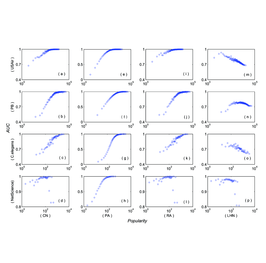
Figure 1: The dependence of algorithmic accuracy on the popularity of links. The results for four typical indices, namely CN, PA, RA and LHN are shown respectively in four columns. Each subgraph is obtained by averaging over 100 implementations with independently random partitions into training set and probe set. The probe set contains 5% of observed links. Note that, the AUC value corresponds to the average AUC of links with the same popularity. The statistics are conducted with log-bin of popularity.

We further investigate the average popularity of the top-$L$ predicted links of different algorithms. In principle, a link prediction algorithm provides a descending ordered list of all non-observed links (i.e., $U\backslash E^{P}$ in our experiment) according to their scores, of which we only focus on the top-$L$ links. Then, the top-$L$ popularity is defined as the average popularity of links among the top-$L$ places. A low top-$L$ average popularity indicates that the algorithm tends to rank the missing links connecting low-degree nodes at the top places. Table 3 shows the top-$L$ popularity of ten local similarity indices on C.elegans network. For CN, PA, AA and RA indices the top-100 popularity scores are extremely high, lager than 100, and the scores will decrease with the increasing of $L$. This indicates that these four indices tend to rank the popular links at the top places. For the other six indices, namely Salton, Jaccard, Sørensen, HPI, HDI and LHN, the top-100 popularity scores are very low. Especially the score of LHN index is very small, approximate to zero, and will increase with the increasing of $L$, suggesting that the LHN index is likely to assign higher scores to the links among whose two endpoints there is at least one node with degree equal to 1. When $L$ is large, the overlap of two ranking lists generated by two algorithms is very high, and thus leads to similar top-$L$ popularity scores. This result further demonstrates that LHN index is more competent to uncover the unpopular links, especially the links with very low-degree nodes.

Table 3: Algorithmic novelty of all local similarity indices on C.elegans, measured by the top-$L$ popularity. Sal, Jac and Sør are the abbreviations for Salton, Jaccard and Sørensen methods respectively. Each number is obtained by averaging 100 implementations with independently random divisions into training set and probe set. The probe set contains 5% of observed links. Here $L$= 100, 500, 1000, 5000, 10000, 20000.

$L$	CN	Sal	Jac	Sør	HPI	HDI	LHN	PA	AA	RA
100	136.7	6.603	9.880	9.880	0.271	14.43	0.000	119.3	147.5	139.9
500	48.23	5.285	7.946	7.947	1.756	9.405	0.006	47.69	51.89	48.89
1000	30.97	6.766	8.759	8.759	0.878	9.507	0.035	30.62	32.80	31.29
5000	9.761	5.427	5.367	5.367	6.574	4.838	0.628	9.483	9.956	9.973
10000	5.397	4.475	4.018	4.018	4.770	3.544	1.383	5.197	5.421	5.453
20000	2.819	2.749	2.687	2.687	2.791	2.652	2.637	2.786	2.819	2.819

3.3 Results for Cold Probe Set

We employ the new partition method to prepare the probe set for experiments. Here we set $D=10$. Thus, we obtain ten different probe sets $E_{i}^{P}$ ($i=1,\cdots,10$). Clearly, each probe set contains 5% of observed links, and $\langle\mathrm{pop}\rangle_{1}<\langle\mathrm{pop}\rangle_{2}<\cdots<\langle\mathrm{pop}\rangle_{10}$. The algorithmic performances on C.elegans network for different probe sets are shown in Table 4. The results for other three networks are similar.

Table 4: Algorithmic accuracies on C.elegans for different probe sets, measured by the AUC value. Sal, Jac and Sør are the abbreviations for Salton, Jaccard and Sørensen methods respectively. Each value is obtained by averaging over 100 implementations with independently divisions of training set and probe set using new partitioning method. The average popularity of these ten probe sets are shown in the brackets. The average popularity of the whole set is 523. The highest AUC value in each row is emphasized in black.

Probe Sets	CN	Sal	Jac	Sør	HPI	HDI	LHN	PA	AA	RA
$E_{1}^{P}$ (57)	0.615	0.724	0.723	0.722	0.713	0.710	0.755	0.247	0.634	0.653
$E_{2}^{P}$ (110)	0.735	0.775	0.780	0.779	0.758	0.778	0.787	0.435	0.756	0.772
$E_{3}^{P}$ (158)	0.754	0.754	0.759	0.759	0.745	0.758	0.748	0.584	0.777	0.791
$E_{4}^{P}$ (211)	0.823	0.799	0.806	0.806	0.782	0.805	0.768	0.708	0.842	0.849
$E_{5}^{P}$ (283)	0.829	0.777	0.780	0.781	0.773	0.782	0.732	0.806	0.854	0.864
$E_{6}^{P}$ (372)	0.867	0.798	0.800	0.800	0.793	0.800	0.726	0.881	0.884	0.884
$E_{7}^{P}$ (493)	0.910	0.813	0.807	0.807	0.819	0.797	0.707	0.929	0.921	0.916
$E_{8}^{P}$ (650)	0.929	0.818	0.801	0.801	0.846	0.769	0.684	0.956	0.934	0.923
$E_{9}^{P}$ (939)	0.943	0.821	0.800	0.800	0.857	0.771	0.669	0.980	0.948	0.939
$E_{10}^{P}$ (1987)	0.947	0.814	0.797	0.797	0.848	0.777	0.649	0.995	0.959	0.965

Compared with other nine indices, LHN has the best performance for predicting the very unpopular links (the links in $E_{1}^{P}$ and $E_{2}^{P}$), while has the worst performance on the links in the probe sets with $P\geq 5$, especially the popular links in $E_{8}^{P}$, $E_{9}^{P}$ and $E_{10}^{P}$. On contrary, PA index gives very good predictions on the popular links, while extremely bad predictions on the links with low-degree nodes where the accuracy is even much lower than the random case. In the middle region where the average popularity is close to that of the randomly selected probe set, RA index outperforms others, which is in accordance with the conclusion in previous studies [14, 36, 37].

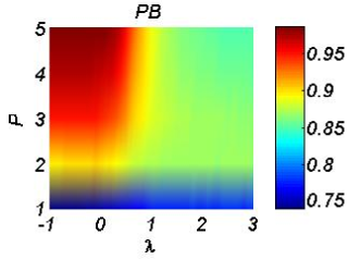
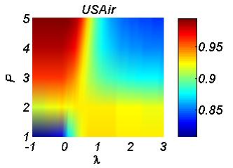
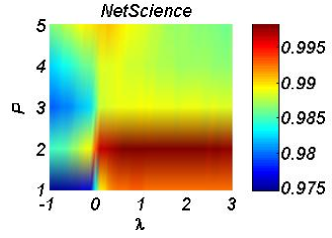
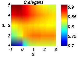
Figure 2: The dependence of AUC on different $\lambda$ and $P$. These results are obtained by averaging over 100 implementations with independently divisions of training set and probe set (by the new partitioning method introduced in Sec. II-C and Sec. III-C). Here we set $D=10$.

4 Improved Index

To design a method for effectively predicting both popular and unpopular links, we propose a parameter-dependent index, which is defined as:

$$s_{xy}=\frac{|\Gamma_{x}\cap\Gamma_{y}|}{(k_{x}\times k_{y})^{\lambda}},$$ (2)

where $\lambda$ is a free parameter. This index is also neighborhood-based and requires only the information of the nearest neighbors, and thus no extra calculational complexity arises. Clearly, when $\lambda$ = 0, this index degenerates to CN, and for the cases $\lambda$ = 0.5 and 1, this index respectively degenerates to the Salton index and LHN index. Given a network, one can tune $\lambda$ to find its optimal value subject to the highest accuracy.

We apply the new index to respectively predict the links in $E_{i}^{P}$ ($i=1,\cdots,10$). The results of four example networks in the ($\lambda$,$P$) plane are shown in Fig. 2 where we focus on the unpopular links ($i=1,\cdots,5$) and $P=i$ means that $E_{i}^{P}$ is employed as the probe set. The results show that the optimal $\lambda$ is positive when $P$ is small (i.e., $P$ = 1,2), while it becomes negative for large $P$. For NetScience $\lambda^{*}$ becomes negative for $P=6$. The dependence of optimal parameter $\lambda^{*}$ on $P$ is shown in Fig. 3. Overall speaking, the optimal parameters $\lambda^{*}$ of four networks are negatively correlated with $P$. In other word, the index with higher (positive) $\lambda$ gives better predictions on unpopular links, while the index with lower (negative) $\lambda$ is good at predicting popular links. For example in C.elegans network, when $P=1$, namely the probe set is constituted with unpopular links, the optimal $\lambda^{*}=2.2$, indicating that to depress the scores of popular links is a better choice, while for $P=10$, namely the probe set is constituted with popular links, the optimal $\lambda^{*}\approx-3$, which indicates that we had better assign higher score to the popular links.

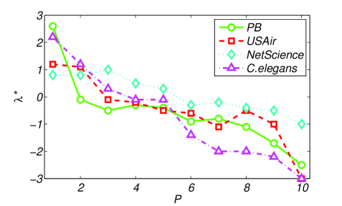
Figure 3: The dependence of the optimal parameter $\lambda^{*}$ on $P$. The probe set contains 5% of the known links. Each value is obtained by averaging the results of 100 independently implementations.

The algorithmic accuracies of ten local similarity indices as well as the proposed index for predicting unpopular links in $E_{1}^{P}$ (i.e., $P=1$) are shown in Table 5. Among the investigated ten local similarity indices, LHN outperforms others for predicting unpopular links. However, the proposed index can improve the accuracy with a proper $\lambda$ which are all positive for all these four networks. Especially, the improvements on PB and C.elegans networks are significant, respectively 10.8% and 8.6% compared with LHN.

Table 5: Comparison of algorithmic accuracy (AUC) on the cold probe set ($P=1$). NS, CE and PB are the abbreviations for NetScience, C.elegans and Political Blogs networks respectively. Sal, Jac and Sør are short for Salton, Jaccard and Sørensen methods. For each network, the probe set contains 5% of the known links. Each value is obtained by averaging over 100 independently implementations. The entries corresponding to the highest accuracies are emphasized in black. For the proposed index, the AUC values are corresponding to the optimal parameters which are shown in the brackets.

Datasets	CN	Sal	Jac	Sør	HPI	HDI	LHN	PA	AA	RA	New
PB	0.649	0.674	0.664	0.664	0.690	0.662	0.701	0.584	0.656	0.664	0.777(2.6)
USAir	0.742	0.888	0.881	0.880	0.831	0.875	0.903	0.370	0.792	0.818	0.928(1.2)
NS	0.973	0.991	0.991	0.991	0.988	0.990	0.992	0.095	0.980	0.981	0.993(0.8)
CE	0.615	0.724	0.723	0.723	0.713	0.709	0.756	0.247	0.633	0.654	0.821(2.2)

5 Experiments on Real Sampling Methods

Table 6: Average popularities of missing links corresponding to different sampling methods. 80% and 90% means the proportion $|E^{T}|/|E|$.

	PB		USAir		NS		CE
	80%	90%	80%	90%	80%	90%	80%	90%
Acquaintance sampling	9674.7	11543.4	3115.2	3662.8	84.3	105.3	854.7	1030.9
Random-walk sampling	5361.1	5220.3	1658.2	1563.6	49.4	41.0	507.7	501.1
Path-based sampling	4505.1	4405.3	1158.4	958.1	18.7	18.0	344.4	296.6

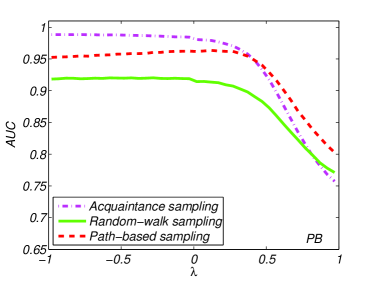
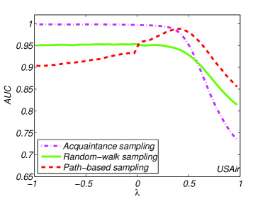
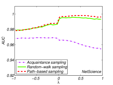
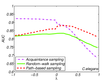
Figure 4: Algorithmic performance of the improved index (see Eq. 2) for the three real sampling methods with different values of $\lambda$. The training set contains 90% of observed links.

To connect our study to the real sampled networks, in this section, we will test the improved index on some real sampling methods. Firstly, we introduce four mainstream sampling methods as follows.

The first one is called snowball sampling (i.e., spider sampling or breadth first sampling, see Ref. [38]), which is a non-probability technique and gets widely used in the studies of World Wide Webs and large-scale social networks. In the beginning of this method, we randomly select one or a few nodes that consist of the initial sampled set, and then we crawl all the neighbors of the nodes in the sampled set, and put them into the sampled set. This process keeps on until a required number of nodes are sampled out. Obviously, it is not relevant for the link prediction problem because this method only leaves missing nodes rather than missing links.

The second one, called acquaintance sampling, is motivated by epidemic immunization with lack of information [39]. In this method, at each time step, a random link of a randomly selected node is sampled out (i.e., being put into the training set) until a required number of links have already been selected. Considering a link $(x,y)$, if it is not yet sampled out, the probability it will be selected at this time step is $\frac{1}{N}(\frac{1}{k_{x}}+\frac{1}{k_{y}})$. Although a link with lower popularity is not necessarily with high $\frac{1}{k_{x}}+\frac{1}{k_{y}}$, statistically speaking, the probability $\frac{1}{N}(\frac{1}{k_{x}}+\frac{1}{k_{y}})$ is negatively correlated with the popularity $(k_{x}-1)(k_{y}-1)$. To our knowledge, this method is a very special method where unpopular links are more likely to be sampled out yet the popular links consist of the probe set.

The third one is named random-walk sampling [40]. A simple way adopted is as follows: (i) initialize a particle on a randomly selected node; (ii) this particle jumps to a randomly selected neighbor and the corresponding link will be added into the training set (i.e., sampled out); (iii) repeat (ii) until a certain number of links have been sampled out, and the rest links compose the probe set. It is well-known that the distribution of visiting frequency of a random walker on a connected network will soon converges to the degree distribution, namely the probability at a certain time step the random walker locate in a node $x$, say $\psi(x)$, is equal to $\frac{k_{x}}{2M}$, where $2M=\sum_{y}k_{y}$ serves as a normalization factor. Considering a link $(x,y)$, if it is not yet sampled out, the probability it will be selected at this time step is $\psi(x)\frac{1}{k_{x}}+\psi(y)\frac{1}{k_{y}}=\frac{1}{M}$. That is to say, the average popularity of links in the probe set is approximately the same to that from the random sampling (we have checked it by simulation). However, the random-walk sampling is not the same as random sampling, for example, the sampled network from the former is always connected yet the one from the latter may contain several components.

The last one is called path-based sampling, which has been applied in extracting the topology of Internet at router level (http://www.routerviews.org). Indeed, this method tracks the transmission of information packets in the Internet, and a link passed by more packets has higher probability to be sampled out. To simulate this process, at each time step, we randomly select a starting point and an end, and we assume that a packet will go from the starting point to the end through a randomly selected shortest path. After a sufficiently large number of time steps, a link with more than a threshold, $N_{T}$, packets will be put into the training set while others compose the probe set. Here for simplicity, we set $N_{T}=1$. Under this method, the links with high betweenness centrality (betweenness centrality quantifies the traffic load of a link, depending on the routing strategy of packet transmission [41]) are favored. Since the popularity of a link is strongly positively correlated with its betweenness centrality on shortest-path routing, the average popularity of links in the probe set is lower than that of the random sampling.

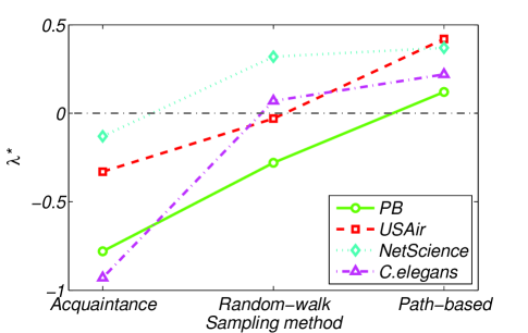
Figure 5: The optimal values of $\lambda$ for the three sampling methods. The dash line denotes $\lambda=0$ as an eye guidance.

The average popularities of missing links corresponding to different sampling methods are shown in Table 6. Agreeing with our analysis, the average popularities of the links in the probe set obeys the inequality $\langle\texttt{pop}\rangle_{acquaintance}>\langle\texttt{pop}\rangle_{random-walk}>\langle\texttt{pop}\rangle_{path-based}$. Figure 4 reports the algorithmic performance (measured by the AUC value) for different sampling methods and different $\lambda$. Very clearly, aiming to predict popular links (e.g., under acquaintance sampling) $\lambda^{*}$ is negative while to predict cold links, $\lambda^{*}$ is positive. In fact, there is strongly negative correlation between the average popularity of links in the probe set and the optimal value of lambda. As shown in Figure 5, where we order the three sampling methods with decreasing average popularity of missing links and thus a positive correlation is observed.

6 Conclusion and discussion

To our knowledge, in the previous studies on link prediction [1], the data sets are always divided in a random manner. Inspired by the in-depth thought about the features of missing links, this article challenges such a straightforward method. Applying a simple measure on link popularity, we propose a method to sample less popular links for probe set. Experimental analysis shows a surprising result that the LHN index performs the best, although it was known to be one of the worst indices if the probe set is a random sampling of all links. We propose a similarity index with a free parameter $\lambda$, by tuning which this index can degenerate to the Common Neighbor index, the Salton index and the LHN index. The optimal value of $\lambda$ monotonously depends on the average link popularity of probe set. We further test this index on three real sampling methods. Agreeing with the main results from theoretical analysis, the optimal value of $\lambda$ increases with the decreasing of the average popularity of links in the probe set. Again, the improved index in a well-tuned range can outperform others under real sampling methods.

Notice that, the main contribution of this article does not lie on the proposed index. Instead, the significance of this work is to raise the serious question about how to properly determine the probe set. To us, this is a very important yet completely ignored problem in information filtering. The reconsideration of dataset division will largely change the understanding and thus the design of algorithms in information filtering (also relevant to the so-called recommendation problem [42]). As a start point, we give a naive method and a preliminary analysis, which is of course far from an satisfied answer to the question. In fact, we think in-depth understanding of real sampling methods may shed light on this issue.

ACKNOWLEDEMENTS

This work is partially supported by the National Natural Science Foundation of China under Grant Nos. 11075031 and 10635040, the Swiss National Science Foundation under Grant No. 200020-132253, and the Fundamental Research Funds for the Central Universities.

References

References

- [1] L. Lü and T. Zhou, Link prediction in complex networks: A survey, 2011 Physica A 390, 1150
- [2] L. Getoor and C. P. Diehl, Link Ming: A Survey, 2005 ACM SIGKDD Explorations Newsletter 7, 3
- [3] H. Yu et al., High-Quality Binary Protein Interaction Map of the Yeast Interactome Network, 2008 Science, 322, 104
- [4] M. P. H. Stumpf, T. Thorne, E. de Silva, R. Stewart, H. J. An, M. Lappe, and C. Wiuf, Estimating the size of the human interactome, 2008 Proc. Natl. Acad. Sci. U.S.A. 105, 6959
- [5] L. A. N. Amaral, A truer measure of our ignorance, 2008 Proc. Natl. Acad. Sci. U.S.A. 105, 6795
- [6] G. Kossinets, Effects of missing data in social networks, 2006 Soc. Networks 28, 247
- [7] J. W. Neal, ”Kracking” the Missing Data Problem: Applying Krackhardt’s Cognitive Social Structures to School-Based Social Networks, 2008 Soc. Educ. 81, 140
- [8] C. von Mering, R. Krause, B. Snel, M. Cornell, S. G. Oliver, S. Field, and P. Bork, Comparative assessment of large-scale data sets of protein-protein interactions, 2002 Nature 417, 399
- [9] C. T. Butts, Network inference, error, and information (in)accuracy: A Bayesian approach, 2003 Soc. Networks 25, 103
- [10] R. Guimerà and M. Sales-Pardo, Missing and spurious interactions and the reconstruction of complex networks, 2009 Proc. Natl. Acad. Sci. U.S.A. 106, 22073
- [11] H.-K. Liu, L. Lü, and T. Zhou, Empirical study of Chinese city airline network, 2007 Acta Physica Sinica 56, 106
- [12] Q.-M. Zhang, M.-S. Shang, and L. Lü, Similarity-based classification in partially labeled networks, 2010 Int. J. Mod. Phys. C 21, 813
- [13] E. A. Leicht, P. Holme and M. E. J. Newman, Vertex similarity in networks, 2006 Phys. Rev. E 73, 026120
- [14] T. Zhou, L. Lü and Y.-C. Zhang, Predicting missing links via local information, 2009 Eur. Phys. J. B 71, 623
- [15] J. A. Hanely and B. J. McNeil, The meaning and use of the area under a receiver operating characteristic (ROC) curve, 1982 Radiology, 143, 29
- [16] D. Liben-Nowell and J. Kleinberg, The Link-Prediction Problem for Social Networks, 2007 J. Am. Soc. Inform. Sci. Technol. 58, 1019
- [17] L. Lü, C.-H. Jin and T. Zhou, Similarity index based on local paths for link prediction of complex networks, 2009 Phys. Rev. E 80, 046122
- [18] G. Salton and M. J. McGill, Introduction to Modern Information Retrieval, (MuGraw-Hill, Auckland, 1983)
- [19] P. Jaccard, Étude comparative de la distribution florale dans une portion des Alpes et des Jura, 1901 Bulletin de la Societe Vaudoise des Science Naturelles 37, 547
- [20] T. Sørensen, A method of establishing groups of equal amplitude in plant sociology based on similarity of species content and its application to analyses of the vegetation on Danish commons, 1948 Biol. Skr. 5, 1
- [21] E. Ravasz, A. L. Somera, D. A. Mongru, Z. N. Oltvai and A.-L. Barábasi, Community structure in social and biological networks, 2002 Science 297, 1553
- [22] A.-L. Barabási and R. Albert, Emergence of Scaling in Random Networks, 1999 Science 286, 509
- [23] Z. Huang, X. Li and H. Chen, Link prediction approach to collaborative filtering, Proceedings of the 5th ACM/IEEECS joint conference on Digital libraries (ACM, NewYork, 2005)
- [24] L. A. Adamic and E. Adar, Friends and neighbors on the Web, 2003 Soc. Networks 25, 211
- [25] Q. Ou, Y.-D. Jin, T. Zhou, B.-H. Wang, and B.-Q. Yin, Power-law strength-degree correlation from resource-allocation dynamics on weighted networks, 2007 Phys. Rev. E 75, 021102
- [26] V. Batageli and A. Mrvar, Pajek Datasets, available at http://vlado.fmf.uni-lj.si/pub/networks/data/default.htm.
- [27] M. E. J. Newman, Finding community structure in networks using the eigenvectors of matrices, 2006 Phys. Rev. E 74, 036104
- [28] D. J. Watts and S. H. Strogatz, Collective dynamics of. ’small-world’ networks, 1998 Nature 393, 440
- [29] R. Ackland, Mapping the US political blogosphere:Are conservative bloggers more prominent, Presentation to BlogTalk Downunder, Sydney, 2005, available at http://incsub.org/blogtalk/images/robertackland.pdf.
- [30] R. Albert and A.-L. Barábasi, Statistical mechanics of complex networks, 2002 Rev. Mod. Phys. 74, 1
- [31] S. N. Dorogovtsev and J. F. F. Mendes, Evolution of networks, 2002 Adv. Phys. 51, 1079
- [32] M. E. J. Newman, The structure and function of complex networks, 2003 SIAM Rev. 45, 167
- [33] S. Boccaletti, V. Latora, Y. Moreno, M. Chavez and D.-U. Huang, Complex networks: structure and dynamics, 2006 Phys. Rep. 424, 175
- [34] L. da F. Costa, F. A. Rodrigues, G. Travieso and P. R. U. Boas, Characterization of complex networks: A survey of measurements, 2007 Adv. Phys. 56, 167
- [35] M. E. J. Newman, Assortative mixing in networks, 2007 Phys. Rev. Lett. 89, 208701
- [36] L. Lü and T. Zhou, Link prediction in weighted networks: The role of weak ties, 2010 EPL 89, 18001
- [37] W. Liu and L. Lü, Link prediction based on local random walk, 2010 EPL 89, 58007
- [38] P. Biernacki and D. Waldorf, Snowball sampling: Problems and techniques of chain referral sampling, 1981 Sociological Methods and Research 10, 141
- [39] R. Cohen, S. Havlin and D. ben-Avraham, Efficient Immunization Strategies for Computer Networks and Populations, 2003 Phys. Rev. Lett. 91, 247901
- [40] L. Lovász, Random walks on graphs: A survey 1993 Combinatorics 2, 1
- [41] G. Yan, T. Zhou, B. Hu, Z.-Q. Fu and B.-H. Wang, Efficient routing on complex networks 2006 Phys. Rev. E 73, 046108
- [42] T. Zhou, Z. Kusckis, J.-G. Liu, M. Medo, J. R. Wakeling, and Y.-C. Zhang, Solving the apparent diversity-accuracy dilemma of recommender systems, 2010 Proc. Natl. Acad. Sci. U.S.A. 107, 4511