On eigenvalues of the Schrödinger operator with an even complex-valued polynomial potential

Abstract.

In this paper, we generalize several results of the article “Analytic continuation of eigenvalues of a quartic oscillator” of A. Eremenko and A. Gabrielov.

We consider a family of eigenvalue problems for a Schrödinger equation with even polynomial potentials of arbitrary degree $d$ with complex coefficients, and $k<(d+2)/2$ boundary conditions. We show that the spectral determinant in this case consists of two components, containing even and odd eigenvalues respectively.

In the case with $k=(d+2)/2$ boundary conditions, we show that the corresponding parameter space consists of infinitely many connected components.

1. Introduction

We study the problem of analytic continuation of eigenvalues of the Schrödinger operator with an even complex-valued polynomial potential, that is, analytic continuation of $\lambda=\lambda(\alpha)$ in the differential equation

(1) $$-y^{\prime\prime}+P_{\alpha}(z)y=\lambda y,$$

where $\alpha=(\alpha_{2},\alpha_{4},\dots,\alpha_{d-2})$ and $P_{\alpha}(z)$ is the even polynomial

$$P_{\alpha}(z)=z^{d}+\alpha_{d-2}z^{d-2}+\dots+\alpha_{2}z^{2}.$$

The boundary conditions for (1) are as follows: Set $n=d+2$ and divide the plane into $n$ disjoint open sectors

$$S_{j}=\{z\in\mathbf{C}\setminus\{0\}:|\arg z-2\pi j/n|<\pi/n\},\quad j=0,1,2,\dots,n-1.$$

The index $j$ should be considered mod $n.$ These are the Stokes sectors of the equation (1). A solution $y$ of (1) satisfies $y(z)\rightarrow 0$ or $y(z)\rightarrow\infty$ as $z\rightarrow\infty$ along each ray from the origin in $S_{j},$ see [Sib75]. The solution $y$ is called subdominant in the first case, and dominant in the second case.

The main result of this paper is as follows:

Theorem 1.

Let $\nu=d/2+1$ and let $J=\{j_{1},j_{2},\dots,j_{2m}\}$ with $j_{k+m}=j_{k}+\nu$ and $|j_{p}-j_{q}|>1$ for $p\neq q.$ Let $\Sigma$ be the set of all $(\alpha,\lambda)\in\mathbf{C}^{\nu}$ for which the equation $-y^{\prime\prime}+(P_{\alpha}-\lambda)y=0$ has a solution with with the boundrary conditions

(2) $$y\text{ is }\text{ subdominant in }S_{j}\mbox{ for all }j\in J$$

where $P_{\mathbf{\alpha}}(z)$ is an even polynomial of degree $d.$ For $m<\nu/2,$ $\Sigma$ consists of two irreducible connected components. For $m=\nu/2,$ which can only happen when $d\equiv 2\mod 4,$ $\Sigma$ consists of infinitely many connected components, distinguished by the number of zeros of the corresponding solution to (1).

1.1. Previous results

The first study of analytic continuation of $\lambda$ in the complex $\beta$-plane for the problem

$$-y^{\prime\prime}+(\beta z^{4}+z^{2})y=\lambda y,\quad y(-\infty)=y(\infty)=0$$

was done by Bender and Wu [BW69], They discovered the connectivity of the sets of odd and even eigenvalues, rigorous results was later proved in [Sim70].

In [EG09a], the even quartic potential $P_{a}(z)=z^{4}+az^{2}$ and the boundary value problem

$$-y^{\prime\prime}+(z^{4}+az^{2})y=\lambda_{a}y,\quad y(\infty)=y(-\infty)=0$$

was considered.

The problem has discrete real spectrum for real $a,$ with $\lambda_{1}<\lambda_{2}<\dots\rightarrow+\infty.$ There are two families of eigenvalues, those with even index and those with odd. If $\lambda_{j}$ and $\lambda_{k}$ are two eigenvalues in the same family, then $\lambda_{k}$ can be obtained from $\lambda_{j}$ by analytic continuation in the complex $\alpha\mathchar 45\relax$plane. Similar results have been found for other potentials, such as the PT-symmetric cubic, where $P_{\alpha}(z)=(iz^{3}+i\alpha z),$ with $y(z)\rightarrow 0,$ as $z\rightarrow\pm\infty$ on the real line. See for example [EG09b].

1.2. Acknowledgements

The author would like to thank Andrei Gabrielov for the introduction to this area of research, and for enlightening suggestions and improvements to the text. Great thanks to Boris Shapiro, my advisor.

2. Preliminaries on general theory of solutions to the Schroedinger equation

We will review some properties for the Schrödinger equation with a general polynomial potential. In particular, these properties hold for an even polynomial potential. These properties may also be found in [EG09a, AG10].

The general Schroedinger equation is given by

(3) $$-y^{\prime\prime}+P_{\alpha}(z)y=\lambda y,$$

where $\alpha=(\alpha_{1},\alpha_{2},\dots,\alpha_{d-1})$ and $P_{\alpha}(z)$ is the polynomial

$$P_{\alpha}(z)=z^{d}+\alpha_{d-1}z^{d-1}+\dots+\alpha_{1}z.$$

We have the associated Stokes sectors

$$S_{j}=\{z\in\mathbf{C}\setminus\{0\}:|\arg z-2\pi j/n|<\pi/n\},\quad j=0,1,2,\dots,n-1,$$

where $n=d+2,$ and index considered mod $n.$ The boundary conditions to (3) are of the form

(4) $$y\mbox{ is subdominant in }S_{j_{1}},S_{j_{2}},\dots,S_{j_{k}}$$

with $|j_{p}-j_{q}|>1$ for all $p\neq q.$

Notice that any solution $y\neq 0$ of (3) is an entire function, and the ratio $f=y/y_{1}$ of any two linearly independent solutions of (3) is a meromorphic function with the following properties, (see [Sib75]).

1. For any $j,$ there is a solution $y$ of (3) subdominant in the Stokes sector $S_{j},$ where $y$ is unique up to multiplication by a non-zero constant.

2. For any Stokes sector $S_{j}$, we have $f(z)\rightarrow w\in\bar{\mathbf{C}}$ as $z\to\infty$ along any ray in $S_{j}$. This value $w$ is called the asymptotic value of $f$ in $S_{j}$.

3. For any $j$, the asymptotic values of $f$ in $S_{j}$ and $S_{j+1}$ (index still taken modulo $n$) are distinct. Furthermore, $f$ has at least 3 distinct asymptotic values.

4. The asymptotic value of $f$ in $S_{j}$ is zero if and only if $y$ is subdominant in $S_{j}.$ We call such sector subdominant for $f$ as well. Note that the boundary conditions given in (4) imply that sectors $S_{j_{1}},\dots,S_{j_{k}}$ are subdominant for $f$ when $y$ is an eigenfunction of (3), (4).

5. $f$ does not have critical points, hence $f:\mathbf{C}\rightarrow\bar{\mathbf{C}}$ is unramified outside the asymptotic values.

6. The Schwartzian derivative $S_{f}$ of $f$ given by

   $$S_{f}=\frac{f^{\prime\prime\prime}}{f^{\prime}}-\frac{3}{2}\left(\frac{f^{\prime\prime}}{f^{\prime}}\right)^{2}$$

   equals $-2(P_{\alpha}-\lambda).$ Therefore one can recover $P_{\alpha}$ and $\lambda$ from $f$.

From now on, $f$ denotes the ratio of two linearly independent solutions of (3), (4).

2.1. Cell decompositions

As above, set $n=\deg P+2$ where $P$ is our polynomial potential and assume that all non-zero asymptotic values of $f$ are distinct and finite. Let $w_{j}$ be the asymptotic values of $f$ with an arbitrary ordering satisfying the only restriction that if $S_{j}$ is subdominant, then $w_{j}=0.$ One can denote by $w_{j}$ the asymptotic value in the Stokes sector $S_{j},$ which will be called the standard order, see section 2.3.

Consider the cell decomposition $\Psi_{0}$ of $\bar{\mathbf{C}}_{w}$ shown in Fig. 1a. It consists of closed directed loops $\gamma_{j}$ starting and ending at $\infty,$ where the index is considered mod $n,$ and $\gamma_{j}$ is defined only if $w_{j}\neq 0.$ The loops $\gamma_{j}$ only intersect at $\infty$ and have no self-intersection other than $\infty.$ Each loop $\gamma_{j}$ contains a single non-zero asymptotic value $w_{j}$ of $f.$ For example, for even $n,$ the boundary condition $y\rightarrow 0$ as $z\rightarrow\pm\infty$ for $z\in\mathbf{R}$ implies that $w_{0}=w_{n/2}=0,$ so there are no loops $\gamma_{0}$ and $\gamma_{n/2}.$ We have a natural cyclic order of the asymptotic values, namely the order in which a small circle around $\infty$ traversed counterclockwise intersects the associated loops $\gamma_{j},$ see Fig. 1a.

We use the same index for the asymptotic values and the loops, so define

$$j_{+}=j+k\text{ where }k\in\{1,2\}\text{ is the smallest integer such that }w_{j+k}\neq 0.$$

Thus, $\gamma_{j_{+}}$ is the loop around the next to $w_{j}$ (in the cyclic order mod $n$) non-zero asymptotic value. Similarly, $\gamma_{j_{-}}$ is the loop around the previous non-zero asymptotic value.

(a) (a) $\Psi_{0}$

(b) (b) $A_{j}(\Psi_{0}).$

Figure 1. Permuting $w_{j}$ and $w_{j_{+}}$ in $\Psi_{0}.$

2.2. From cell decompositions to graphs

Proofs of all statements in this subsection can be found in [EG09a].

Given $f$ and $\Psi_{0}$ as above, consider the preimage $\Phi_{0}=f^{-1}(\Psi_{0}).$ Then $\Phi_{0}$ gives a cell decomposition of the plane $\mathbf{C}_{z}.$ Its vertices are the poles of $f$ and the edges are preimages of the loops $\gamma_{j}.$ An edge that is a preimage of $\gamma_{j}$ is labeled by $j$ and called a $j\mathchar 45\relax$edge. The edges are directed, their orientation is induced from the orientation of the loops $\gamma_{j}$. Removing all loops of $\Phi_{0},$ we obtain an infinite, directed planar graph $\Gamma,$ without loops. Vertices of $\Gamma$ are poles of $f,$ each bounded connected component of $\mathbf{C}\setminus\Gamma$ contains one simple zero of $f,$ and each zero of $f$ belongs to one such bounded connected component. There are at most two edges of $\Gamma$ connecting any two of its vertices. Replacing each such pair of edges with a single undirected edge and making all other edges undirected, we obtain an undirected graph $T_{\Gamma}.$ It has no loops or multiple edges, and the transformation from $\Phi_{0}$ to $T_{\Gamma}$ can be uniquely reversed.

A junction is a vertex of $\Gamma$ (and of $T_{\Gamma}$) at which the degree of $T_{\Gamma}$ is at least 3. From now on, $\Gamma$ refers to both the directed graph without loops and the associated cell decomposition $\Phi_{0}$.

2.3. The standard order of asymptotic values

For a potential $P$ of degree $d,$ the graph $\Gamma$ has $n=d+2$ infinite branches and $n$ unbounded faces corresponding to the Stokes sectors of $P$. We fixed earlier the ordering $w_{0},w_{1},\dots,w_{n-1}$ of the asymptotic values of $f.$

If each $w_{j}$ is the asymptotic value in the sector $S_{j},$ we say that the asymptotic values have the standard order and the corresponding cell decomposition $\Gamma$ is a standard graph.

Lemma 2 (See Prop. 6 [EG09a]).

If a cell decomposition $\Gamma$ is a standard graph, then the corresponding undirected graph $T_{\Gamma}$ is a tree.

In the next section, we define some actions on $\Psi_{0}$ that permute non-zero asymptotic values. Each unbounded face of $\Gamma$ (and $T_{\Gamma}$) will be labeled by the asymptotic value in the corresponding Stokes sector. For example, labeling an unbounded face corresponding to $S_{k}$ with $w_{j}$ or just with the index $j,$ indicates that $w_{j}$ is the asymptotic value in $S_{k}.$

From the definition of the loops $\gamma_{j},$ a face corresponding to a dominant sector has the same label as any edge bounding that face. The label in a face corresponding to a subdominant sector $S_{k}$ is always $k,$ since the actions defined below only permute non-zero asymptotic values.

An unbounded face of $\Gamma$ is called (sub)dominant if the corresponding Stokes sector is (sub)dominant.

2.4. Properties of graphs and their face labeling

Lemma 3 (See Section 3 in [EG09a]).

Any graph $\Gamma$ have the following properties:

1. Two bounded faces of $\Gamma$ cannot have a common edge, (since a $j\mathchar 45\relax$edge is always at the boundary of an unbounded face labeled $j.$)

2. The edges of a bounded face of a graph $\Gamma$ are directed clockwise, and their labels increase in that order. Therefore, a bounded face of $T_{\Gamma}$ can only appear if the order of $w_{j}$ is non-standard.

3. Each label appears at most once in the boundary of any bounded face of $\Gamma.$

4. The unbounded faces of $\Gamma$ adjacent to a junction $u,$ always have the labels cyclically increasing counterclockwise around $u.$

5. The boundary of a dominant face labeled $j$ consists of infinitely many directed $j\mathchar 45\relax$edges, oriented counterclockwise around the face.

6. If $w_{j}=0$ there are no $j\mathchar 45\relax$edges.

7. Each vertex of $\Gamma$ has even degree, since each vertex in $\Phi_{0}=f^{-1}(\Psi_{0})$ has even degree, and removing loops to obtain $\Gamma$ preserves this property.

Following the direction of the $j\mathchar 45\relax$edges, the first vertex that is connected to an edge labeled ${j_{+}}$ is the vertex where the $j\mathchar 45\relax$edges and the ${j_{+}}\mathchar 45\relax$edges meet. The last such vertex is where they separate. These vertices, if they exist, must be junctions.

Definition 4.

Let $\Gamma$ be a standard graph, and let $j\in\Gamma$ be a junction where the $j\mathchar 45\relax$edges and $j_{+}\mathchar 45\relax$edges separate. Such junction is called a $j\mathchar 45\relax$junction.

There can be at most one $j\mathchar 45\relax$junction in $\Gamma,$ the existence of two or more such junctions would violate property (III) of the face labeling. However, the same junction can be a $j\mathchar 45\relax$junction for different values of $j.$

There are three different types of $j\mathchar 45\relax$junctions, see Fig. 2.

(a) (a)

(b) (b)

(c) (c)

Figure 2. Different types of $j\mathchar 45\relax$junctions.

Case (a) only appears when $w_{j+1}\neq 0.$ Cases (b) and (c) can only appear when $w_{j+1}=0.$ In (c), the $j\mathchar 45\relax$edges and $j_{+}\mathchar 45\relax$edges meet and separate at different junctions, while in (b), this happens at the same junction.

Definition 5.

Let $\Gamma$ be a standard graph with a $j\mathchar 45\relax$junction $u$. A structure at the $j\mathchar 45\relax$junction is the subgraph $\Xi$ of $\Gamma$ consisting of the following elements:

• The edges labeled $j$ that appear before $u$ following the $j\mathchar 45\relax$edges.

• The edges labeled $j_{+}$ that appear after $u$ following the $j_{+}\mathchar 45\relax$edges.

• All vertices the above edges are connected to.

If $u$ is as in Fig. 2a, $\Xi$ is called an $I\mathchar 45\relax$structure at the $j\mathchar 45\relax$junction. If $u$ is as in Fig. 2b, $\Xi$ is called a $V\mathchar 45\relax$structure at the $j\mathchar 45\relax$junction. If $u$ is as in Fig. 2c, $\Xi$ is called a $Y\mathchar 45\relax$structure at the $j\mathchar 45\relax$junction.

Since there can be at most one $j\mathchar 45\relax$junction, there can be at most one structure at the $j\mathchar 45\relax$junction.

A graph $\Gamma$ shown in Fig. 3 has one (dotted) $I\mathchar 45\relax$structure at the $1\mathchar 45\relax$junction $v,$ one (dotted) $I\mathchar 45\relax$structure at the $4\mathchar 45\relax$junction $u,$ one (dashed) $V\mathchar 45\relax$structure at the $2\mathchar 45\relax$junction $v$ and one (dotdashed) $Y\mathchar 45\relax$structure at the $5\mathchar 45\relax$junction $u$.

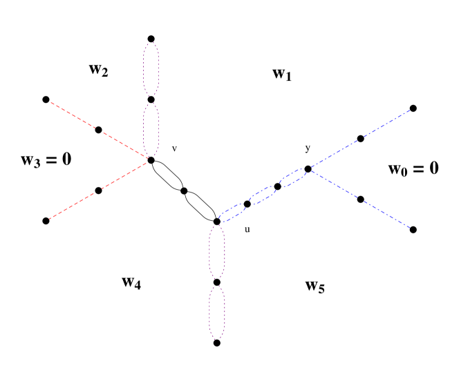
Figure 3. Graph $\Gamma$ with (dotted) $I\mathchar 45\relax$structures, a (dashed) $Y\mathchar 45\relax$structure and a (dotdashed) $Y\mathchar 45\relax$structure.

Note that the $Y\mathchar 45\relax$structure is the only kind of structure that contains an additional junction. We refer to such additional junctions as $Y\mathchar 45\relax$junctions. For example, the junction marked $y$ in Fig. 3 is a $Y\mathchar 45\relax$junction.

2.5. Braid actions on graphs

As in [AG10], we define continuous deformations $A_{j}$ of the loops in Fig. 1a, such that the new loops are given in terms of the old ones by

$$A_{j}(\gamma_{k})=\begin{cases}\gamma_{j}\gamma_{j_{+}}\gamma_{j}^{-1}\text{ if }k=j\\ \gamma_{j}\text{ if }k=j_{+}\\ \gamma_{k}\text{ otherwise }\end{cases},\quad A_{j}^{-1}(\gamma_{k})=\begin{cases}\gamma_{j_{+}}\text{ if }k=j\\ \gamma_{j_{+}}^{-1}\gamma_{j}\gamma_{j_{+}}\text{ if }k=j_{+}\\ \gamma_{k}\text{ otherwise }\end{cases}$$

These actions, together with their inverses, generate the Hurwitz (or sphere) braid group $\mathcal{H}_{m},$ where $m$ is the number of non-zero asymptotic values. (For a definition of this group, see [LZ04].) The action of the generators $A_{j}$ and $A_{k}$ commute if $|j-k|\geq 2.$

The property (V) of the eigenfunctions implies that each $A_{j}$ induces a monodromy transformation of the cell decomposition $\Phi_{0},$ and of the associated directed graph $\Gamma.$

3. Properties of even actions on centrally symmetric graphs

3.1. Additional properties for even potential

In addition to the previous properties for general polynomials, these additional properties holds for even polynomial potentials $P$ (see [EG09a]). From now until the end of the article, $\nu=(\deg(P)+2)/2.$

Each solution $y$ of (1) is either even or odd and we may choose $y$ and $y_{1}$ such that $f=y/y_{1}$ is odd.

If the asymptotic values $w_{0},w_{1},\dots,w_{2\nu-1}$ are ordered in the standard order, we have that $w_{j}=-w_{j+\nu}.$

We may choose the loops centrally symmetric in Fig. 1a which implies that $\Phi_{0}$ and $\Gamma$ are centrally symmetric.

3.2. Even braid actions

Define the even actions $E_{j}$ as $E_{j}=A_{j}\circ A_{j+\nu}.$

Assume that $\Gamma$ is a graph with the property that if $w_{j}$ is the asymptotic value in $S_{k},$ then $w_{j+n}$ is the asymptotic value in $S_{k+\nu}.$ (For example, all standard graphs have this property, with $j=k.$) It follows from the symmetric property of $E_{j}$ that $E_{j}$ preserves this property. To illustrate, we have that $E_{j}(\Psi_{0})$ is given in Fig. 4.

Figure 4. $E_{j}(\Psi_{0})$

Lemma 6.

If $\Gamma$ is centrally symmetric, then $E_{j}(\Gamma)$ and $E_{j}^{-1}(\Gamma)$ are centrally symmetric graphs.

Proof.

We may choose the deformations of the paths $\gamma_{j}$ and $\gamma_{j+\nu}$ being centrally symmetric, which implies that the composition $A_{j}\circ A_{j+\nu}$ preserves the property of $\Gamma$ being centrally symmetric, see details in [EG09a]. ∎

Lemma 7.

Let $\Gamma$ be a centrally symmetric standard graph with no $j\mathchar 45\relax$junction. Then $E_{j}^{2}(\Gamma)=\Gamma.$

Proof.

Since $A_{j}$ and $A_{j+n}$ commute, we have that $E_{j}^{2}=A_{j}^{2}A_{j+\nu}^{2},$ and the statement then follows from [AG10, Lemma 12]. ∎

Theorem 8.

Let $\Gamma$ be a centrally symmetric standard graph with a $j\mathchar 45\relax$junction $u.$ Then $E_{j}^{2}(\Gamma)\neq\Gamma,$ and the structure at the $j\mathchar 45\relax$junction is moved one step in the direction of the $j\mathchar 45\relax$edges under $E_{j}^{2}.$ The inverse of $E^{2}_{j}$ moves the structure at the $j\mathchar 45\relax$junction one step backwards along the $j_{+}\mathchar 45\relax$edges.

Since $\Gamma$ is centrally symmetric, it also has a $j+\nu\mathchar 45\relax$junction, and the structure at the $j+\nu\mathchar 45\relax$junction is moved one step in the direction of the $j+n\mathchar 45\relax$edges under $E_{j}^{2}.$ The inverse of $E^{2}_{j}$ moves the structure at the $j+\nu\mathchar 45\relax$junction one step backwards along the $(j+\nu)_{+}\mathchar 45\relax$edges.

Proof.

Since $E_{j}^{2}=A_{j}^{2}A_{j+\nu}^{2},$ the result follows from [AG10, Theorem 13]. ∎

4. Proving Main Theorem 1

Notice that each centrally symmetric standard graph $\Gamma$ has either a vertex in its center, or a double edge, connecting two vertices. This property follows from the fact that $\Gamma_{T}$ is a centrally symmetric tree.

Lemma 9.

Let $\Gamma$ be a centrally symmetric graph. Then for every action $E_{j},$ $\Gamma$ has a vertex at the center iff $E_{j}(\Gamma)$ has a vertex at the center.

Proof.

This is evident from the definition of the actions, since the action only changes the edges, and preserves the vertices. ∎

Corollary 10.

The spectral determinant has at least two connected components.

Each centrally symmetric standard graph $\Gamma$ is of one of two types:

1. $\Gamma$ has a central double edge. The vertices of the central double edge are called root junctions.

2. $\Gamma$ has a junction at its center. This junction is called the root junction $u_{r}.$

Definition 11.

A centrally symmetric standard graph $\Gamma$ is in ivy form if $\Gamma$ consists of structures connected to one or two root junctions.

Definition 12.

Let $\Gamma$ be a centrally symmetric standard graph.

The root metric of $\Gamma,$ denoted $|\Gamma|_{r}$ is defined as

$$|\Gamma|_{r}=\sum_{v\in\Gamma}\left(\deg(v)-2\right)|v-u_{r}|$$

where the sum is taken over all vertices $v$ of $\Gamma_{1}.$ Here $deg(v)$ is the total degree of the vertex $v$ in $T_{\Gamma}$ and $|v-u_{r}|$ is the length of the shortest path from $v$ to the closest root junction $u_{r}$ in $T_{\Gamma}.$

Lemma 13.

The graph $\Gamma$ is in ivy form if and only if all but its root junctions are $Y\mathchar 45\relax$junctions.

Proof.

This follows from the definitions of the structures. ∎

Theorem 14.

Let $\Gamma$ be a centrally symmetric standard graph. Then there is a sequence of even actions $E^{*}=E_{j_{1}}^{\pm 2},E_{j_{2}}^{\pm 2},\dots,$ such that $E^{*}(\Gamma)$ is in ivy form.

Proof.

Assume that $\Gamma$ is not in ivy form.

Let $U$ be the set of junctions in $\Gamma$ that are not $Y\mathchar 45\relax$junctions. Since $\Gamma$ is not in ivy form we have that $|U|\geq 3.$ Let $u_{r}\neq u_{1}$ be two junctions in $U$ such that $|u_{r}-u_{1}|$ is maximal, and $u_{r}$ is the central junction closest to $u_{1}.$ Let $p$ be the path from $u_{r}$ to $u_{1}$ in $T_{\Gamma}.$ It is unique since $T_{\Gamma}$ is a tree. Let $v$ be the vertex preceding $u_{1}$ on the path $p.$ The edge from $v$ to $u_{1}$ in $T_{\Gamma}$ is adjacent to at least one dominant face with label $j$ such that $w_{j}\neq 0.$ Therefore, there exists a $j\mathchar 45\relax$edge between $v$ and $u_{1}$ in $\Gamma.$ Suppose first that this $j\mathchar 45\relax$edge is directed from $u_{1}$ to $v.$ Let us show that in this case $u_{1}$ must be a $j\mathchar 45\relax$junction, i.e., the dominant face labeled $j_{+}$ is adjacent to $u_{1}$.

Since $u_{1}$ is not a $Y\mathchar 45\relax$junction, there is a dominant face adjacent to $u_{1}$ with a label $k\neq j,j_{+}$. Hence no vertices of $p$, except possibly $u_{1}$ can be adjacent to $j_{+}\mathchar 45\relax$edges. If $u_{1}$ is not a $j\mathchar 45\relax$junction, there are no $j_{+}\mathchar 45\relax$edges adjacent to $u_{1}$. This implies that any vertex of $\Gamma$ adjacent to a $j_{+}\mathchar 45\relax$edge is further away from $u_{r}$ than $u_{1}$.

Let $u_{2}$ be the closest to $u_{1}$ vertex of $\Gamma$ adjacent to a $j_{+}\mathchar 45\relax$edge. Then $u_{2}$ should be a junction of $T_{\Gamma}$, since there are two $j_{+}\mathchar 45\relax$edges adjacent to $u_{2}$ in $\Gamma$ and at least one more vertex (on the path from $u_{1}$ to $u_{2}$) which is connected to $u_{2}$ by edges with labels other than $j_{+}$. Since $u_{2}$ is further away from $u_{r}$ that $u_{1}$ and the path $p$ is maximal, $u_{2}$ must be a $Y\mathchar 45\relax$junction. If the $j\mathchar 45\relax$edges and $j_{+}\mathchar 45\relax$edges would meet at $u_{2}$, $u_{1}$ would be a $j\mathchar 45\relax$junction. Otherwise, a subdominant face labeled $j+1$ would be adjacent to both $u_{1}$ and $u_{2}$, while a subdominant face adjacent to a $Y\mathchar 45\relax$junction cannot be adjacent to any other junctions.

Hence $u_{1}$ must be a $j\mathchar 45\relax$junction. By Theorem 8, the action $E_{j}^{2}$ moves the structure at the $j\mathchar 45\relax$junction $u_{1}$ one step closer to $u_{r}$ along the path $p,$ and similarly happens on the opposite side of $\Gamma,$ decreasing $|\Gamma|_{c}$ by at least 2.

The case when the $j\mathchar 45\relax$edge is directed from $v$ to $u_{1}$ is treated similarly. In that case, $u_{1}$ must be a $j_{-}\mathchar 45\relax$junction, and the action $A_{j_{-}}^{-2}$ moves the structure at the $j_{-}\mathchar 45\relax$junction $u_{1}$ one step closer to $u_{r}$ along the path $p.$

We have proved that if $|U|>1$ then $|\Gamma|_{r}$ can be reduced. Since it is a non-negative integer, after finitely many steps we must reach a stage where $U$ consists only of the root junctions. Hence $E^{*}(\Gamma)$ is in ivy form. ∎

The above Theorem shows that for every centrally symmetric standard graph $\Gamma,$ there is a sequence of actions that turns $\Gamma$ into ivy form. A graph in ivy form consists of one or two root junctions, with attached structures. These structures can be ordered counterclockwise around each root junction. These observations motivates the following lemmas:

Lemma 15.

Let $\Gamma$ be a centrally symmetric standard graph, and let $u_{r}\in\Gamma$ be a root junction of type $j_{-}$ and of type $j.$ Let $S_{1}$ and $S_{2}$ be the corresponding structures attached to $u_{r}.$

1. If $S_{1}$ and $S_{2}$ are of type $Y$ resp. $V,$ then there is a sequence of even actions that interchange these structures.

2. If $S_{1}$ and $S_{2}$ are of type $I$ resp. $Y,$ then there is a sequence of even actions that converts the type $Y$ structure to a type $V$ structure.

3. If $S_{1}$ and $S_{2}$ are both of type $Y,$ then there is a sequence of even actions that converts one of the $Y\mathchar 45\relax$structures to a $V\mathchar 45\relax$structure.

Proof.

By symmetry, there are identical structures in $\Gamma$ attached to a root junction of type $n+j_{-}$ and $n+j,$ with attached structures $S^{\prime}_{1}$ and $S^{\prime}_{2}$ of the same type as $S_{1}$ resp. $S_{2}.$

Lemma 19, 20 and 22 in [AG10], gives the existence of a non-even sequence of actions, that only acts on $S_{1}$ and $S_{2}$ in the desired way.

In all these cases, the sequence is of the form

$$A^{*}=A_{k_{1}}^{\pm 2}A_{k_{2}}^{\pm 2}\dots A_{k_{m}}^{\pm 2}$$

where $k_{1},k_{2},\dots k_{m}\in\{j,j_{-}\}.$ It follows that the action

$$B^{*}=A_{k_{1}+\nu}^{\pm 2}A_{k_{2}+\nu}^{\pm 2}\dots A_{k_{m}+\nu}^{\pm 2}$$

do the same as $A^{*}$ but on $S^{\prime}_{1}$ and $S^{\prime}_{2}.$

Now, $E^{*}=A^{*}\circ B^{*}$ is even, since by commutativity, it is equal to

$$(A_{k_{1}}^{\pm 2}A_{k_{1}+\nu}^{\pm 2})(A_{k_{2}}^{\pm 2}A_{k_{2}+\nu}^{\pm 2})\dots(A_{k_{m}}^{\pm 2}A_{k_{m}+\nu}^{\pm 2})$$

which easily may be written in terms of our even actions as

$$E_{k_{1}}^{\pm 2}E_{k_{2}}^{\pm 2}\dots E_{k_{m}}^{\pm 2}.$$

This sequence of actions has the desired property. ∎

Corollary 16.

Let $\Gamma$ be a centrally symmetric graph, with two adjacent dominant faces. Then there is a sequence of even actions $E^{*}$ such that $E^{*}(\Gamma)$ has either one or two junctions.

Proof.

We may apply even actions to make $\Gamma$ into a standard graph, and then convert it to ivy form. The condition that we have two dominant faces, is equivalent to existence of $I\mathchar 45\relax$structures. If there are no $Y\mathchar 45\relax$structures, then the only junctions of $\Gamma$ are the root junctions, and we are done. Otherwise, we may the $Y\mathchar 45\relax$ and $V\mathchar 45\relax$structures, so that a $Y\mathchar 45\relax$structure appears next to the $I\mathchar 45\relax$structure. By using the second part of the above lemma, we decrease the number of $Y\mathchar 45\relax$structures of $\Gamma$ by two. After a finite number of actions, we arrive at a graph in ivy form without $Y\mathchar 45\relax$structures. ∎

Lemma 17.

Let $\Gamma$ be a centrally symmetric graph, with no adjacent dominant faces. Then there is a sequence of even actions $E^{*}$ such that $E^{*}(\Gamma)$ is in ivy form, with at most two $Y\mathchar 45\relax$structures.

Proof.

By Teorem 14, we may assume that $\Gamma$ is in ivy form. Since there are no adjacent dominant sectors, the only structures of $\Gamma$ are of $Y$ and $V$ type. These are attached to the one or two root junctions.

Assume that there are more than two $Y\mathchar 45\relax$structures present. Two of these must be attached to the same root junction, $u_{r}.$ By repeatedly applying part one of Lemma 15, we may interchange the $Y\mathchar 45\relax$ and $V\mathchar 45\relax$structures attached to $u_{r}$ such that the two $Y\mathchar 45\relax$structures are adjacent. Applying part three of Lemma 15, we may then convert one of the two $Y\mathchar 45\relax$structures to a $V\mathchar 45\relax$structure.

By symmetry, the same change is done on the opposite side of $\Gamma$ and total number of $Y\mathchar 45\relax$structures of $\Gamma$ have therefore been reduced by two. We may repeat this procedure a finite number of times, until the number of $Y\mathchar 45\relax$structures is less than three. This implies the lemma. ∎

Lemma 18 (See [AG10]).

Let $\Gamma$ be a standard graph such that no two dominant faces are adjacent. Then the number of bounded faces of $\Gamma$ is finite and does not change after any action $A_{j}^{2}$.

Corollary 19.

The number of bounded faces of $\Gamma$ does not change under any even action $E_{j}^{2}=A_{j}^{2}A_{j+\nu}^{2}.$

Lemma 20.

Let $\nu=n/2=d/2+1$ and let $\Sigma$ be the space of all $(\alpha,\lambda)\in\mathbf{C}^{\nu-1}$ such that equation (1) admits a solution subdominant in non-adjacent Stokes sectors

(5) $$S_{j_{1}},S_{j_{2}},\dots,S_{2m}$$

with $j_{k+m}=j_{k}+\nu$ and $1\leq m\leq\nu/2.$ Then $\Sigma$ is a smooth complex analytic submanifold of $\mathbf{C}^{\nu-1}$ of the codimension $m.$

Proof.

We consider the space $\mathbf{C}^{\nu-1}$ as a subspace of the space $\mathbf{C}^{n-2}$ of all $(\alpha,\lambda)$ corresponding to the general polynomial potentials in (3), with $\alpha=(\alpha_{1},\dots,\alpha_{d-1})$. Let $f$ be a ratio of two linearly independent solutions of (3), and let $w=(w_{0},\dots,w_{n-1})$ be the set of the asymptotic values of $f$ in the Stokes sectors $S_{0},\dots,S_{n-1}$.

Then $w$ belongs to the subset $Z$ of ${\bar{\mathbf{C}}}^{n-1}$ where the values $w_{j}$ in adjacent Stokes sectors are distinct and there are at least three distinct values among $w_{j}$. The group $G$ of fractional-linear transformations of $\bar{\mathbf{C}}$ acts on $Z$ diagonally, and the quotient $Z/G$ is a $(n-3)$-dimensional complex manifold.

Theorem 7.2, [Bak77] implies that the mapping $W:\mathbf{C}^{n-2}\to Z/G$ assigning to $(\alpha,\lambda)$ the equivalence class of $w$ is submersive. More precisely, $W$ is locally invertible on the subset $\{\alpha_{d-1}=0\}$ of $\mathbf{C}^{n-2}$

For an even potential, there exists an odd function $f.$ The corresponding set of asymptotic values satisfies $\nu$ linear conditions $w_{j+\nu}=-w_{j}$ for $j=0,\dots,\nu-1$. For $(\alpha,\lambda)\in\Sigma$, we can assume that $S_{j_{1}},\dots,S_{j_{m}}$ are subdominant sectors for $f$. This adds $m$ linearly independent conditions $w_{j_{1}}=\dots=w_{j_{m}}=0.$ Let $Z_{0}$ be the corresponding subset of $Z$. Its codimension in $Z$ is $\nu+m$. The one-dimensional subgroup $\mathbf{C}^{*}$ of $G$ consisting of multiplications by non-zero complex numbers preserves $Z_{0}$, and $gZ_{0}\cap Z_{0}=\emptyset$ for each $g\in G\setminus\mathbf{C}^{*}$. The explaination is as follows:

Since we have at least two subdominant sectors, only fractional linear transforms that preserves 0 are allowed. Furthermore, there exists a sector $S_{k}$ with the value $w_{k}$ different from 0 and $\infty$ (otherwise we would have only two asymptotic values). There is a unique transformation, multiplication by $w_{k}^{-1}$, preserving 0 and sending $\pm w_{k}$ to $\pm 1$. This implies that the only transformation preserving 0 and sending $\pm w_{k}$ to another pair of opposite numbers is multiplication by a non-zero constant.

Hence $GZ_{0}$ is a $G$-invariant submanifold of $Z$ of codimension $\nu+m-2$, and its image $Y_{0}\subset Y$ is a smooth submanifold of codimension $\nu+m-2$. Due to Bakken’s theorem, $W^{-1}(Y_{0})$ intersected with the $(n-3)$-dimensional space of $(\alpha,\lambda)$ with $\alpha_{d-1}=0$ is a smooth submanifold of codimension $\nu+m-2$, dimension $\nu-m-1$. Accordingly, it is a smooth submanifold of codimension $m$ of the space $\mathbf{C}^{\nu-1}$. ∎

Proposition 21.

Let $\Sigma$ be as in Lemma 20. If at least two adjacent Stokes sectors are missing in (5), then $\Sigma$ consists of two irreducible complex analytic manifolds.

Proof.

Nevanlinna theory (see [Nev32, Nev53]), implies that, for each symmetric standard graph $\Gamma$ with the properties listed in Lemma 3, there exists $(\alpha,\lambda)\in\mathbf{C}^{n-1}$ and an odd meromorphic function $f(z)$ such that $f$ is the ratio of two linearly independent solutions of (1) with the asymptotic values $w_{j}$ in the Stokes sectors $S_{j}$, and $\Gamma$ is the graph corresponding to the cell decomposition $\Phi_{0}=f^{-1}(\Psi_{0})$. This function, and the corresponding point $(\alpha,\lambda)$ is defined uniquely.

Let $W:\Sigma\to Y_{0}$ be as in the proof of Lemma 20. Then $\Sigma$ is an unramified covering of $Y_{0}$. Its fiber over the equivalence class of $w\in Y_{0}$ consists of the points $(\alpha_{\Gamma},\lambda_{\Gamma})$ for all standard graphs $\Gamma$. Each action $A_{j}^{2}$ corresponds to a closed loop in $Y_{0}$ starting and ending at $w$. It should be noted that $Y_{0}$ is a connected manifold. Since for a given list of subdominant sectors a standard graph with one vertex is unique, Theorem 15 implies that the monodromy group has two orbits; odd and even eigenfunctions cannot be exchanged by any path in $Y_{0}$, while any odd (even) can be transferred into any other odd (even) eigenfunction by a sequence of $E_{k}^{\pm 2}$.

Hence $\Sigma$ consists of two irreducible connected components (see, e.g., [Kho04]). ∎

This immediately implies Theorem 1, for $m<\nu/2.$ The following propostion implies the case where $m=\nu/2.$

Proposition 22.

Let $\Sigma$ be the space of all $(\alpha,\lambda)\in\mathbf{C}^{\nu-1}$, for even $\nu,$ such that equation (1) admits a solution subdominant in every other Stokes sector, that is, in $S_{0},S_{2},\dots,S_{n-2}.$

Then irreducible components $\Sigma_{k},$ $k=0,\,1,\dots$ of $\Sigma$, which are also its connected components, are in one-to-one correspondence with the sets of centrally symmetric standard graphs with $k$ bounded faces. The corresponding solution of (1) has $k$ zeros and can be represented as $Q(z)e^{\phi(z)}$ where $Q$ is a polynomial of degree $k$ and $\phi$ a polynomial of degree $(d+2)/2$.

Proof.

Let us choose $w$ and $\Psi_{0}$ as in the proof of Proposition 21. Repeating the arguments in the proof of Proposition 21, we obtain an unramified covering $W:\Sigma\to Y_{0}$ such that its fiber over $w$ consists of the points $(\alpha_{\Gamma},\lambda_{\Gamma})$ for all standard graphs $\Gamma$ with the properties listed in Lemma 3.

Since we have no adjacent dominant sectors, Lemma 17 implies that any standard graph $\Gamma$ can be transformed by the monodromy action to a graph $\Gamma_{0}$ in ivy form with at most two $Y$-structures attached at the root junction(s) of type $j$ and $j+\nu.$

Lemma 18 implies that $\Gamma$ and $\Gamma_{0}$ have the same number $k$ of bounded faces. If $k=0$, the graph $\Gamma_{0}$ is unique. If $k>0$, the graph $\Gamma_{0}$ is completely determined by $k.$ Hence for each $k=0,1,\dots$ there is a unique orbit of the monodromy group action on the fiber of $W$ over $w$ consisting of all standard graphs $\Gamma$ with $k$ bounded faces. This implies that $\Sigma$ has one irreducible component for each $k$.

Since $\Sigma$ is smooth by Lemma 20, its irreducible components are also its connected components.

Finally, let $f_{\Gamma}=y/y_{1}$ where $y$ is an odd solution of (1) subdominant in the Stokes sectors $S_{0},S_{2},\dots,S_{n-2}$. Then the zeros of $f$ and $y$ are the same, each such zero belongs to a bounded domain of $\Gamma$, and each bounded domain of $\Gamma$ contains a single zero. Hence $y$ has exactly $k$ simple zeros. Let $Q$ be a polynomial of degree $k$ with the same zeros as $y$. Then $y/Q$ is an entire function of finite order without zeros, hence $y/Q=e^{\phi}$ where $\phi$ is a polynomial. Since $y/Q$ is subdominant in $(d+2)/2$ sectors, $\deg\phi=(d+2)/2$. ∎

5. Illustrating example

We will now give a small example on how to apply the method given in the previous section, Theorem 14 and Lemma 15. Let $\Gamma$ be as in Fig. 5a. From subsection 2.4, we have that a dominant face with label $j$ have $j\mathchar 45\relax$edges as boundaries. Hence the faces $0$ and $4$ are subdominant. Also, the direction of the edges are directed counterclockwise in each of the dominant faces.

(a) (a)

(b) (b)

Figure 5. The graphs $\Gamma$ and $E_{1}^{2}(\Gamma)$

Applying $E_{1}^{2},$ moves the $I\mathchar 45\relax$structure at the $1\mathchar 45\relax$junction one step to the right, following the $1\mathchar 45\relax$edges. Similarly, the $I\mathchar 45\relax$structure at the $5\mathchar 45\relax$junction moves one step to the left. Therefore, $E_{1}^{2}(\Gamma)$ is given in Fig. 5b. The graph $E_{1}^{2}(\Gamma)$ is now in ivy form, it consists of a center junction connected to four $I\mathchar 45\relax$structures and two $Y\mathchar 45\relax$structures. We proceed by using the algorithm in Lemma 15, and apply $E_{1}^{2}$ two times more. These steps are given in Fig. 6.

(a) (a)

(b) (b)

Figure 6. The graphs $E_{1}^{4}(\Gamma)$ and $E_{1}^{6}(\Gamma)$

The next step in the lemma is to move the newly created $V\mathchar 45\relax$structures to the center junction. We therefore apply $E_{3}^{2}$ two times. These final steps are presented in Fig. 7, and we have reached the unique graph with only one junction.

(a) (a)

(b) (b)

Figure 7. The graphs $E_{3}^{2}E_{1}^{6}(\Gamma)$ and $E_{3}^{4}E_{1}^{6}(\Gamma)$

References

- [AG10] P. Alexandersson and A. Gabrielov. On eigenvalues of the schrödinger operator with a polynomial potential with complex coefficients. 2010.
- [Bak77] I. Bakken. A multiparameter eigenvalue problem in the complex plane. Amer. J. Math., 99(5):1015–1044, 1977.
- [BW69] C. Bender and T. Wu. Anharmonic oscillator. Phys. Rev. (2), 184:1231–1260, 1969.
- [EG09a] A. Eremenko and A. Gabrielov. Analytic continuation of egienvalues of a quartic oscillator. Comm. Math. Phys., 287(2):431–457, 2009.
- [EG09b] A. Eremenko and A. Gabrielov. Irreducibility of some spectral determinants. 2009. arXiv:0904.1714.
- [Kho04] A. G. Khovanskii. On the solvability and unsolvability of equations in explicit form. (russian). Uspekhi Mat. Nauk, 59(4):69–146, 2004. translation in Russian Math. Surveys 59 (2004), no. 4, 661–736.
- [LZ04] S. Lando and A. Zvonkin. Graphs on Surfaces and Their Applications. Springer-Verlag, 2004.
- [Nev32] R. Nevanlinna. Über Riemannsche Flächen mit endlich vielen Windungspunkten. Acta Math., 58:295–373, 1932.
- [Nev53] R. Nevanlinna. Eindeutige analytische Funktionen. Springer, Berlin, 1953.
- [Sib75] Y. Sibuya. Global theory of a second order differential equation with a polynomial coefficient. North-Holland Publishing Co., Amsterdam-Oxford; American Elsevier Publishing Co., Inc., New York, 1975.
- [Sim70] B. Simon. Coupling constant analyticity for the anharmonic oscillator. Ann. Physics, 58:76–136, 1970.