Eigenvalues of rank one perturbations of unstructured matrices

Abstract.

Let $A$ be a fixed complex matrix and let $u,v$ be two vectors. The eigenvalues of matrices $A+\tau uv^{\top}$ $(\tau\in\mathbb{R})$ form a system of intersecting curves. The dependence of the intersections on the vectors $u,v$ is studied.

Introduction

The motivation for this paper is the following numerical experiment. Take a matrix $A\in\mathbb{C}^{n\times n}$ and nonzero vectors $u,v\in\mathbb{C}^{n}$ and plot the set

(0.1) $$\{\sigma(A+\tau uv^{\top}):\tau\in\mathbb{R}\}.$$

It is well known that above set consists of a finite number of curves, that intersect only in a finite number of points. However, it appears that for $u,v\in\mathbb{C}^{n}$ chosen randomly from a continuous distribution on $\mathbb{C}^{n}$ there are no intersection points except, possibly, the of spectrum of $A$. Furthermore, for all $\tau\in\mathbb{R}\setminus\{0\}$ all eigenvalues of $A+\tau uv^{\top}$, that are not eigenvalue of $A$, are simple. A typical case for $A=J_{3}(0)$ is shown of Figure 1, note that the only intersection of the eigenvalue curves is at $0\in\sigma(A)$. Since it appears that the intersection points outside $\sigma(A)$ are multiple eigenvalues of $A+\tau uv^{\top}$ (cf. Proposition 2.2(ii)), we will be also interested in a problem of existence of multiple eigenvalues of $A+\tau uv^{\top}$ for some $\tau\in\mathbb{C}$.

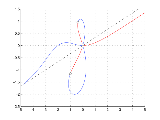
Figure 1. Eigenvalues of $B(\tau)=J_{3}(0)+\tau uv^{\top}$ for $\tau>0$ in red, for $\tau<0$ in blue, see also Remark 4.2.

Some light on the phenomenon of lack of double eigenvalues in the numerical simulations is put by the following marvelous result of Hörmander and Melin [6]. Let the Jordan canonical form of the matrix $A$ be

$$A\cong\bigoplus_{j=1}^{r}\bigoplus_{i=1}^{k_{j}}J_{n_{j,i}}(\lambda_{j}),$$

where the Jordan blocks $J_{n_{j,i}}(\lambda_{j})$ corresponding to each eigenvalue $\lambda_{j}$ ($j=1,\dots r$) are in decreasing order, i.e. $n_{j,1}\geq n_{j,2}\geq\dots\geq n_{j,k_{j}}$. Then for generic $u$ and $v$ (i.e. for all $u$ and $v$ except a ‘small’ set, see Preliminaries) the Jordan form of $A+uv^{\top}$ is the following

$$A+uv^{\top}\cong\bigoplus_{j=1}^{r}\bigoplus_{i=2}^{k_{j}}J_{n_{j,i}}(\lambda_{j})\oplus\bigoplus_{h=1}^{l}J_{1}{\mu_{h}},$$

where $\mu_{h}\neq\mu_{h^{\prime}}$ for $h\neq h^{\prime}$. In other words, for each eigenvalue $\lambda_{j}$ ($j=1,\dots r$) only the largest chain in the Jordan structure is destroyed and there appears a structure of simple eigenvalues instead.

The behavior of eigenvalues of $A+\tau uv^{\top}$ as functions of $\tau$ for small values of $\tau$ is also well known, see, e.g., [10, 18] and [1, 8, 13, 14, 19]. Namely, for small values of $|\tau|$ and for generic $u$ and $v$ for each $j=1,\dots r$ there are $n_{j,1}$ simple eigenvalues $\mu_{j,k}(\tau)$, $k=1,\cdots,n_{j,1}$ of $A+\tau uv^{\top}$ in a punctured neighborhood of $\lambda_{j}$, and they are given by

(0.2) $$\mu_{j,k}(\tau)=\lambda_{j}+\tau^{1/{n_{j,1}}}\cdot\left(c_{j}\right)^{1/n_{j,1}}\cdot\exp\left(\frac{-2\pi ik}{n_{j,1}}\right)+O(\tau^{2/n_{j,1}}),$$

where the number $c_{j}$ can be expressed explicitly in terms of $A,u$ and $v$; see [14], Proposition 1. That is, the eigenvalues $\mu_{j,k}(\tau)$ are approximately given by the roots of the polynomial equation

(0.3) $$(\mu-\lambda_{j})^{n_{j,1}}=\tau\cdot c_{j},\quad j=1,\dots r.$$

However, neither the Hörmander–Mellin result nor the above small $\tau$ asymptotic of eigenvalues does not explain the lack of crossing of eigenvalue curves that appears in numerical simulations. The purpose of the present paper is to show that this behavior is indeed ‘generic’ although the notion of genericity will have some different shades.

For historical reasons let us mention two works prior to the Hörmander–Mellin paper, in [17] the invariant factors of a one–dimensional perturbation are considered and in [9] the perturbation theory for normal matrices is developed. The result by Hörmander–Mellin lay dormant for about a decade before being rediscovered independently by Dopico and Moro [5] and Savchenko [14, 15]. Since that time the interest in topic has grown up, see e.g. [11, 12] for an alternative proof using ideas from systems theory and for perturbation theory for structured matrices. Although the results presented below concern a similar matter the reasonings are independent of the previous work and the content of the paper is self–contained. The main outcome are Theorems 3.1, 4.1, 5.1, 6.1 and 6.2. First four of them allow the parameter $\tau$ to be complex, while in the last one we return to the real parameter $\tau$. This collection gives a complete description of the generic behavior of the set in (0.1).

1. Preliminaries

In this section, we gather some known results which will be the basis for our further investigation. An important technique used in this paper is the resultant. Let

$$q_{1}(\lambda)=a_{n_{1}}\lambda^{n_{1}}+\cdots+a_{0},\qquad q_{2}(\lambda)=b_{n_{2}}\lambda^{n_{2}}+\cdots+b_{0}$$

be two complex polynomials. By $S(q_{1},q_{2})$ we denote the Sylwester resultant matrix of $q_{1}$ and $q_{2}$:

(1.1) $$S(q_{1},q_{2})=\begin{bmatrix}a_{n_{1}}&\cdots&a_{0}&0&\cdots&\cdots&0\\ 0&a_{n_{1}}&\cdots&a_{0}&0&\cdots&0\\ \vdots&&\ddots&&\ddots&&0\\ 0&\cdots&\cdots&0&a_{n_{1}}&\cdots&a_{0}\\ b_{n_{2}}&\cdots&b_{0}&0&\cdots&\cdots&0\\ 0&b_{n_{2}}&\cdots&b_{0}&0&\cdots&0\\ \vdots&&\ddots&&\ddots&&0\\ 0&\cdots&\cdots&0&b_{n_{2}}&\cdots&b_{0}\\ \end{bmatrix}\in\mathbb{C}^{(n_{1}+n_{2})\times(n_{1}+n_{2})}.$$

It is well known that $q_{1}$ and $q_{2}$ have a common root if and only if $\det S(q_{1},q_{2})=0$.

Let $A\in\mathbb{C}^{n\times n}$ and let $u,v\in\mathbb{C}^{n}$. Occasionally we will use the notation

$$B(\tau)=A+\tau uv^{\top},\quad\tau\in\mathbb{C},$$

remembering, nevertheless, that we are interested in the $(u,v)$–dependence of the spectral structure of $B(\tau)$. Recall that an eigenvalue $\lambda_{0}$ of $B\in\mathbb{C}^{n\times n}$ is called non–derogatory if $\dim\ker(B-\lambda_{0})=1$. The following result may be found in [14], Lemma 5, for completeness sake we include a proof.

Lemma 1.1.

Let $A\in\mathbb{C}^{n\times n}$ and let $u,v\in\mathbb{C}^{n}$. Then for all $\tau\in\mathbb{C}\setminus\left\{0\right\}$ all eigenvalues of $B(\tau)$ that are not eigenvalues of $A$ are non-derogatory.

Proof.

Let $\lambda_{0}\in\sigma(B(\tau))\setminus\sigma(A)$ and let $\tau\neq 0$. Using the fact that ${\rm rank\,}(X+Y)\leq{\rm rank\,}X+{\rm rank\,}Y$ for any compatible matrices $X,Y$ we obtain

$$n={\rm rank\,}(A-\lambda_{0}) \leq{\rm rank\,}(A+\tau uv^{\top}-\lambda_{0})+{\rm rank\,}(\tau uv^{\top})=$$

$$={\rm rank\,}(B(\tau)-\lambda_{0})+1,$$

which shows that ${\rm rank\,}(B(\tau)-\lambda_{0})\geq n-1$. Hence $\dim\ker(B(\tau)-\lambda_{0})=1$ and so $\lambda_{0}$ is a non-derogatory eigenvalue of $B(\tau)$. ∎

Following [11] we say that a subset $\Omega$ of $\mathbb{C}^{n}$ is generic if $\Omega$ is not empty and the complement $\mathbb{C}^{n}\setminus\Omega$ is contained in a (complex) algebraic set which is not $\mathbb{C}^{n}$. In such case $\mathbb{C}^{n}\setminus\Omega$ is nowhere dense and of $2n$–dimensional Lebesgue measure zero. We use the phrase for generic $v\in\mathbb{C}^{n}$ as an abbreviation of: ‘there exist a generic $\Omega\subseteq\mathbb{C}^{n}$ such that for all $v\in\Omega$’. Our main results, except Theorem 6.2, have the following form:

• Let $A\in\mathbb{C}^{n\times n}$. Then for generic $u$ and $v$ …,

which should be read formally as

• For every $A\in\mathbb{C}^{n\times n}$ there exists a generic subset $\Omega$ of $\mathbb{C}^{2n}$, possibly dependent on $A$, such that for $(u,v)\in\Omega$….

Most of our reasoning are independent of a choice of basis. Let $T$ be an invertible matrix. Then

$$T(A+\tau uv^{\top})T^{-1}=TAT^{-1}+\tau(Tu)(v^{\top}T^{-1}).$$

In consequence, the Jordan structures of the matrices $A+\tau uv^{\top}$ and $TAT^{-1}+\tau(Tu)(v^{\top}T^{-1})$ are identical. In other words the transformation

(1.2) $$(A,u,v^{\top})\mapsto(TAT^{-1},Tu,v^{\top}T^{-1})$$

preserves the spectral structure of $B(\tau)$ for all $\tau\in\mathbb{R}$. Let $T_{A}$ be the transformation of $A$ to its Jordan canonical form, that is

(1.3) $$A^{\prime}=T_{A}AT_{A}^{-1}=\bigoplus_{j=1}^{r}\bigoplus_{i=1}^{k_{j}}J_{n_{j,i}}(\lambda_{j}),$$

where $J_{k}(\lambda)$ denotes the Jordan block of size $k$ with the diagonal entries equal $\lambda$ and the entries on the first upper–diagonal equal one and

(1.4) $$n_{j,1}\geq n_{j,2}\geq\cdots\geq n_{j,k_{j}},\quad j=1,\dots,r.$$

We will describe now a special instance of the transformation $T$ that consists of two steps, i.e. $T=T_{v}T_{A}$. Let $T_{A}$ be as above, next we decompose $u^{\prime}=T_{A}u$ and $v^{\prime}{}^{\top}=v^{\top}T_{A}^{\top}$ according to the Jordan form of $A^{\prime}$ as follows:

(1.5) $$u^{\prime}=\begin{bmatrix}u^{\prime}_{1}\\ u^{\prime}_{2}\\ \vdots\\ u^{\prime}_{p_{u}}\end{bmatrix},\qquad u^{\prime}_{j}=\begin{bmatrix}u^{\prime}_{j,1}\\ u^{\prime}_{j,2}\\ \vdots\\ u^{\prime}_{j,k_{j}}\end{bmatrix},\qquad u^{\prime}_{j,i}=\begin{bmatrix}u^{\prime}_{j,i,1}\\ u^{\prime}_{j,i,2}\\ \vdots\\ u^{\prime}_{j,i,n_{j,i}}\end{bmatrix}\in\mathbb{C}^{n_{j,i}},$$

and

(1.6) $$v^{\prime}=\begin{bmatrix}v^{\prime}_{1}\\ v^{\prime}_{2}\\ \vdots\\ v^{\prime}_{p_{u}}\end{bmatrix},\qquad v^{\prime}_{j}=\begin{bmatrix}v^{\prime}_{j,1}\\ v^{\prime}_{j,2}\\ \vdots\\ v^{\prime}_{j,k_{j}}\end{bmatrix},\qquad v^{\prime}_{j,i}=\begin{bmatrix}v^{\prime}_{j,i,1}\\ v^{\prime}_{j,i,2}\\ \vdots\\ v^{\prime}_{j,i,n_{j,i}}\end{bmatrix}\in\mathbb{C}^{n_{j,i}}.$$

We put

$$T_{v}=\bigoplus_{j=1}^{r}\bigoplus_{i=1}^{k_{j}}{\rm Toep\,}(v_{j,i}),$$

where by ${\rm Toep\,}(w)$ we denote the $k\times k$ upper-triangular Toeplitz matrix whose first row is given by $w\in\mathbb{C}^{k}$. Obviously $T_{v}$ commutes with $A$. Now note that for generic $v$ one has

(1.7) $$v^{\prime}_{j,i,1}\neq 0\qquad i=1,\dots,k_{j},\ j=1,\dots,r,$$

which implies that $T_{v}$ is invertible, consequently $T_{v}A^{\prime}T_{v}^{-1}=A^{\prime}$. Furthermore, $v^{\prime\prime}{}^{\top}=v^{\prime}{}^{\top}T_{v}^{-1}$ has the following form

(1.8) $$v^{\prime\prime}_{j,i}=\begin{bmatrix}1\\ 0\\ \vdots\\ 0\end{bmatrix}\qquad i=1,\dots,k_{j},\ j=1,\dots,r.$$

The triplet $(TAT^{-1},Tu,v^{\top}T^{-1})$, where $T=T_{v}T_{A}$, will be called the Brunovsky form of $(A,u,v^{\top})$, cf. [2]. Note the following simple lemma, that will allow us to reduce the problem of genericity in $u$ and $v$ to a problem of genericity in $u$ with a fixed $v$.

Lemma 1.2.

If $\Omega_{0}$ is a generic subset of $\mathbb{C}^{n}$ then the set

$$\{(u,v)\in\mathbb{C}^{2n}:T_{v}\text{ is invertible },T_{v}T_{A}u\in\Omega_{0}\}$$

is a generic subset of $\mathbb{C}^{2n}$.

2. The characteristic polynomial of $B(\tau)$

The present section contains the basic tools used in the paper. Namely, we introduce the polynomial $p_{uv}$ and provide a formula for the characteristic polynomial of $B(\tau)$.

The minimal polynomial of $A$ will be denoted by $m(\lambda)$. Everywhere in the paper (1.3) and (1.4) are silently assumed, consequently one has

(2.1) $$m(\lambda)=\prod_{j=1}^{r}(\lambda-\lambda_{j})^{n_{j,1}}.$$

We also put

(2.2) $$p_{uv}(\lambda)=m(\lambda)\cdot v^{\top}(\lambda-A)^{-1}u.$$

Note that $p_{uv}$ is invariant on the transformation (1.2). Transforming $A$ to it Jordan form we easily see that $p_{uv}$ is a polynomial of degree at most $\deg m-1$. The following Lemma plays an essential role in the further reasoning.

Lemma 2.1.

For generic $u$ and $v$ the polynomial $p_{uv}$ is of degree $\deg m-1$ and has no double roots and no common roots with $m$.

Proof.

Using Lemma 1.2 and the fact that $p_{uv}$ is invariant on the transformation (1.2) we may assume that $A$ is in the Brunovsky canonical form and treat $v$ as fixed. For simplicity consider the case when $A$ consists of one Jordan block only, i.e.

$$A=J_{n}(\lambda_{1}),\quad v=\begin{bmatrix}1\\ 0\\ \vdots\\ 0\end{bmatrix},\quad u=\begin{bmatrix}u_{1}\\ u_{2}\\ \vdots\\ u_{n}\end{bmatrix}.$$

Then $m(\lambda)=(\lambda-\lambda_{1})^{n}$ and

$$(\lambda-A)^{-1}={\rm Toep\,}([(\lambda-\lambda_{1})^{-1},(\lambda-\lambda_{1})^{-2},\dots,(\lambda-\lambda_{1})^{-n}]^{\top}).$$

Consequently,

$$p_{uv}(\lambda)=u_{1}(\lambda-\lambda_{1})^{n-1}+\cdots+u_{n-1}(\lambda-\lambda_{1})+u_{n}.$$

Hence, the generic assumption $u_{1}\neq 0$ implies that $\deg p_{uv}=\deg m-1$. Further on, the generic assumption $u_{n}\neq 0$ implies that $p_{u}$ and $m$ do not have common roots. To prove that for generic $u$ the polynomial $p_{uv}$ has simple roots only let us consider the Sylwester resultant matrix $S(p_{uv},p_{uv}^{\prime})$. Note that $\det S(p_{uv},p_{uv}^{\prime})$ is a nonzero polynomial in $u$. Hence, the equation $\det S(p_{uv},p_{uv}^{\prime})=0$ defines a proper algebraic subset of $\mathbb{C}^{n}$.

The general case follows by similar arguments from the equation

$$p_{uv}(\lambda)=m(\lambda)\cdot\sum_{j=1}^{r}\sum_{i=1}^{k_{j}}v_{j,i}^{\top}(\lambda-J_{n_{j,i}}(\lambda_{j}))^{-1}u_{j,i}.$$

∎

We put

$$q(\lambda)=\prod_{i=1}^{r}\prod_{j=2}^{k_{i}}(\lambda-\lambda_{i})^{n_{i,j}}=\frac{\det(\lambda-A)}{m(\lambda)},$$

with the convention $\prod_{2}^{1}:=1$. We also define the family of polynomials $p_{uv,\tau}$ by

(2.3) $$p_{uv,\tau}(\lambda)=m(\lambda)-\tau p_{uv}(\lambda),\quad\tau\in\mathbb{R}.$$

Proposition 2.2.

Let $A\in\mathbb{C}^{n\times n}$, then the following statements hold.

• For every $u,v\in\mathbb{C}^{n}$, $\tau\in\mathbb{C}$ the characteristic polynomial of $A+\tau uv^{\top}$ equals $q\cdot p_{uv,\tau}$.

• For every $u,v\in\mathbb{C}^{n}$, $\tau_{1},\tau_{2}\in\mathbb{C}$ with $\tau_{1}\neq\tau_{2}$ one has

  $$\sigma(A+\tau_{1}uv^{\top})\cap\sigma(A+\tau_{2}uv^{\top})\subseteq\sigma(A).$$

• For generic $u$ and $v$ and all $\tau\in\mathbb{C}\setminus\left\{0\right\}$ there are exactly $\deg m$, counting algebraic multiplicities, eigenvalues of $A+\tau uv^{\top}$ that are not eigenvalues of $A$.

Point (iii) shows that the only crossings of the eigenvalue curves in (0.1) are the multiple eigenvalues of $A+\tau uv^{\top}$ for some $\tau\in\mathbb{R}$.

Proof.

(i) For any $u,v\in\mathbb{C}^{n}$, $\tau\in\mathbb{C}$ and $\lambda\in\mathbb{C}\setminus\sigma(A)$ we have (cf. [14], Lemma 1)

$$\det(\lambda-(A+\tau uv^{\top})) =\det\left((\lambda-A)(I-(\lambda-A)^{-1}\tau uv^{\top})\right)$$

$$=\det(\lambda-A)\det(I-(\lambda-A)^{-1}\tau uv^{\top})$$

$$=\det(\lambda-A)(1-\tau v^{\top}(\lambda-A)^{-1}u)$$

Dividing both sides by $q$ and emploing (2.2) we obtain

(2.4) $$\frac{\det(\lambda-(A+\tau uv^{\top}))}{q(\lambda)}=m(\lambda)-\tau p_{uv}(\lambda),$$

which finishes the proof of (i).

(ii) Assume that $\lambda_{0}\in\sigma(A+\tau_{1}uv^{\top})\cap\sigma(A+\tau_{2}uv^{\top})$ with $\tau_{1}\neq\tau_{2}$. By (i) $\lambda_{0}$ is either a root of $q$, or a common root of the polynomials $p_{uv,\tau_{1}}$ and $p_{uv,\tau_{2}}$. In the former case $\lambda_{0}$ clearly belongs to $\sigma(A)$, in the latter case $\lambda_{0}$ is a root of $(\tau_{1}-\tau_{2})p_{uv}$ and consequently of $m$. Hence, $\lambda_{0}\in\sigma(A)$ as well.

(iii) By Lemma 2.1, for generic $u$ and $v$ and all $\tau\in\mathbb{C}\setminus\left\{0\right\}$ the polynomials $p_{uv,\tau}$ and $m$ do not have common roots and consequently $q$ is the greatest common divisor of the characteristic polynomials of $A$ and $A+\tau uv^{\top}$. Hence, for generic $u$ and $v$ the roots of $p_{uv,\tau}$ are precisely the eigenvalues of $B(\tau)$ which are not eigenvalues of $A$. Since the $\deg p_{uv,\tau}=\deg m$, there are exactly $\deg m$, counting algebraic multiplicities, eigenvalues of $A+\tau uv^{\top}$ which are not eigenvalues of $A$.

∎

Note that by Lemma 1.1 for each $\tau\neq 0$ the eigenvalues in $\sigma(B(\tau)\setminus\sigma(A)$ are non–derogatory. However, the proposition above does not say, that for each $\tau\neq 0$ the eigenvalues in $\sigma(B(\tau)\setminus\sigma(A)$ are simple. Obviously, for a fixed value of $\tau$ and generic $u$ and $v$ the eigenvalues in $\sigma(B(\tau)\setminus\sigma(A)$ are simple, as follows from the Hörmander–Mellin result, but this is a weaker statement.

3. The Jordan structure of $A+\tau uv^{\top}$ at the eigenvalues of $A$.

The theorem below shows that the Jordan structure of $B(\tau)$ at the eigenvalues of $A$ is constant for all $\tau\neq 0$. The technique of the proof was used in [11] to reprove the Hörmander–Mellin result.

Theorem 3.1.

Let $A\in\mathbb{C}^{n\times n}$ and let (1.3), (1.4) be the Jordan form of $A$. Then for generic $u$ and $v$ and all $\tau\in\mathbb{C}\setminus\left\{0\right\}$ the sizes of the Jordan blocks of $A+\tau uv^{\top}$ corresponding to the eigenvalue $\lambda_{j}$ are $n_{j,2}\geq\dots\geq n_{j,k_{j}}$, for $j=1,\ldots,r$.

Proof.

Using the transformation (1.2) we can assume that $A$ is in the Brunovsky canonical form. Denote by $e_{j,l}$ ($j=1,\dots,r$, $l=1,\dots,n_{j,1}+n_{j,2}+\cdots+n_{j,k_{j}}$) the vector with one on the $l$–th position in the $j$–th block and zeros elsewhere. Then the following sequences are Jordan chains of $A+\tau uv^{\top}$ corresponding to the eigenvalue $\lambda_{j}$ ($j=1,\dots r$):

(3.1) $$\begin{array}[]{l}e_{j,1}-e_{j,n_{j,1}+1},\dots,e_{j,n_{j,2}}-e_{j,n_{j,1}+n_{j,2}};\\ e_{j,1}-e_{j,n_{j,1}+n_{j,2}+1},\dots,e_{j,n_{j,3}}-e_{j,n_{j,1}+n_{j,2}+n_{j,3}};\\ \vdots\\ e_{j,1}-e_{j,n_{j,1}+\cdots+n_{j,k_{j}-1}+1},\dots,e_{j,n_{j,k_{j}}}-e_{j,n_{j,1}+\cdots+n_{k_{j}-1}+n_{j,k_{j}}}.\\ \end{array}$$

Hence, we see that for generic $u$ and $v$ there are Jordan chains of $A+\tau uv^{\top}$ of lengths $n_{j,2}\geq\dots\geq n_{j,k_{j}}$ corresponding to the eigenvalue $\lambda_{j}$. (Obviously, if $k_{j}=1$ then $\lambda_{j}$ is not an eigenvalue of $A+\tau uv^{\top}$). By Proposition 2.2 the dimension of the algebraic eigenspace corresponding to $\sigma(B(\tau))\setminus\sigma(A)$ is $\deg m=n_{j,1}+\cdots+n_{r,1}$. Hence, none of the Jordan chains in (3.1) can be extended and the proof is finished. ∎

4. The large $\tau$ asymptotic of eigenvalues of $B(\tau)$.

In this section it is shown that the eigenvalues of $B(\tau)$ that are not eigenvalues of $A$ tend with $\tau\to\infty$ to the roots of the polynomial $p_{uv}$, except one eigenvalue that goes to infinity. This behavior is again generic in $u$ and $v$.

Theorem 4.1.

Let $A\in\mathbb{C}^{n\times n}$. Then for generic $u,v\in\mathbb{C}^{n}$ there exist differentiable functions

$$\mu_{1},\dots,\mu_{l}:\left\{\tau\in\mathbb{C}:|\tau|>\tau_{0}\right\}\to\mathbb{C},$$

with $l=\deg m$ and some $\tau_{0}>0$, such that

• $\sigma(B(\tau))\setminus\sigma(A)=\left\{\mu_{j}(\tau):j=1,\dots,l\right\}$ for $|\tau|>\tau_{0}$;

• $\mu_{j}\neq\mu_{j^{\prime}}$ for $j,j^{\prime}=1,\dots,l$, $j\neq j^{\prime}$;

• $\mu_{1}(\tau),\dots,\mu_{l-1}(\tau)$ tend with $|\tau|\to\infty$ to the $l-1$ roots of the polynomial $p_{uv}$;

• $\mu_{l}(\tau)/\tau\to v^{\top}u$ with $\tau\to\infty$.

The theorem says, in other words, that as $\tau$ goes to $\infty$ the eigenvalues of $B(\tau)$ which are not eigenvalues of $A$ are simple, exactly $l-1$ of them are approximate the roots of $p_{uv}$ and one goes to infinity, asymptotically along the ray in the complex plane going from zero through the number $v^{\top}u$.

Proof.

By Lemma 2.1 there are $l-1$ simple roots of the polynomil $p_{uv}$, let us denote them by $\lambda_{1},\dots,\lambda_{l-1}$. Let $\varepsilon>0$ be such that the closed discs

$$C_{j}(\varepsilon)=\{\lambda\in\mathbb{C}:|\lambda-\lambda_{j}|\leq\varepsilon\},\qquad j=1,\dots l-1$$

do not intersect. Consider the polynomials

$${q}_{\tau}(\lambda)=\frac{1}{\tau}m(\lambda)-p_{uv}(\lambda),\quad\tau>\tau_{0}$$

and observe that $\frac{1}{\tau}m(\lambda)$ converges with $|\tau|\to\infty$ uniformly to zero on $\bigcup_{j=1}^{l-1}C_{j}(\varepsilon)$. By the Rouche theorem there is a $\tau_{0}>0$ so that for $|\tau|>\tau_{0}$ the polynomial $q_{\tau}$ has exactly one simple root $\mu_{j}(\tau)$ in each of the sets $C_{j}(\varepsilon)$, $j=1,\dots,l-1$. Hence, the root $\mu_{l}(\tau)\notin\bigcup_{j=1}^{l-1}C_{j}(\varepsilon)$ is simple as well. By simplicity of the roots we get $q_{\tau}^{\prime}(\mu_{j}(\tau))\neq 0$ for $j=1,\dots l$, $|\tau|>\tau_{0}$. Hence, by implicit function theorem the functions $\mu_{1}(\tau),\dots,\mu_{l}(\tau)$ are differentiable. Recalling that $\sigma(B(\tau))\setminus\sigma(A)$ consists by Proposition 2.2 precisely of the roots of $q_{\tau}(\lambda)$ finishes the proof of (i) and (ii). Letting $\varepsilon\to 0$ we obtain (iii). To prove (iv) note that

$$\sigma\left(\frac{1}{\tau}B(\tau)\right)=\sigma\left(\frac{1}{\tau}A\right)\cup\left\{\frac{\mu_{1}(\tau)}{\tau},\dots,\frac{\mu_{l}(\tau)}{\tau}\right\},\quad|\tau|>\tau_{0}.$$

As $\tau\to\infty$ the matrix $\tau^{-1}B(\tau)$ converges to the rank one matrix $uv^{\top}$ and thus $\mu_{l}(\tau)/\tau$ converges to $v^{\top}u$. ∎

Remark 4.2.

In Figure 1 the roots of the polynomial $p_{uv}$ are marked with black circles, and the asymptotic ray $y=(v^{\top}u)x$ is the dashed line.

5. Triple eigenvalues of $B(\tau)$.

In this section we show that for generic $u,v$ there are no triple eigenvalues in $\sigma(B(\tau))\setminus\sigma(A)$ for all $\tau\in\mathbb{C}$. In particular there are generically no triple crossings of the eigenvalue curves.

Theorem 5.1.

Let $A\in\mathbb{C}^{n\times n}$. Then for generic $u,v\in\mathbb{C}^{n}$ and for all $\tau\in\mathbb{C}$ the algebraic multiplicity of the eigenvalues of $A+\tau uv^{\top}$ that are not eigenvalues of $A$ is at most two.

Proof.

Suppose that $u$ and $v$ are such that for some $\tau\in\mathbb{C}$ the matrix $B(\tau)$ has an eigenvalue $\lambda_{0}\notin\sigma(A)$ of multiplicity at least three. Then by Lemma 1.1 $B(\tau)$ has a Jordan block of size at least three at $\lambda_{0}$. Consequently, by Proposition 2.2, $\lambda_{0}$ is a triple root of $p_{uv,\tau}$, i.e.

$$m(\lambda_{0})-\tau p_{uv}(\lambda_{0}) =0,$$

$$m^{\prime}(\lambda_{0})-\tau p_{uv}^{\prime}(\lambda_{0}) =0,$$

$$m^{\prime\prime}(\lambda_{0})-\tau p_{uv}^{\prime\prime}(\lambda_{0}) =0.$$

Solving for $\tau$ from the first equation and substituting in the second and third we obtain

$$m^{\prime}(\lambda_{0})p_{uv}(\lambda_{0})-m(\lambda_{0})p_{uv}^{\prime}(\lambda_{0})=0,$$

$$m^{\prime\prime}(\lambda_{0})p_{uv}(\lambda_{0})-m(\lambda_{0})p_{uv}^{\prime\prime}(\lambda_{0})=0.$$

Let $s$ be the greatest common divisor of $m$ and $m^{\prime}$. Since $\lambda_{0}$ does not belong to $\sigma(A)$, it is a common root of the polynomials

(5.1) $$f_{uv}= \frac{m^{\prime}}{s}p_{uv}-\frac{m}{s}p_{uv}^{\prime},$$

(5.2) $$g_{uv}= m^{\prime\prime}p_{uv}-mp_{uv}^{\prime\prime}.$$

Therefore, $\det S(f_{uv},g_{uv})=0$. Summarizing, we showed so far that the set of all $u$ and $v$ for which there exists $\tau\in\mathbb{C}$ such that the matrix $B(\tau)$ has an eigenvalue $\lambda_{0}\notin\sigma(A)$ of multiplicity at least three is contained in the set of all $u,v\in\mathbb{C}^{n}$ such that $\det S(f_{uv},g_{uv})=0$. Clearly $\det S(f_{uv},g_{uv})$ is a polynomial in the coordinates of $u$ and $v$. We show now, that it is a nonzero polynomial, i.e. that for some $u,v$ the polynomials $f_{uv}$, $g_{uv}$ do not have a common root, which will finish the proof. First consider the case $\deg m=1$. Then for generic $u,v$ the polynomial $p_{uv}$ is a constant nonzero polynomial and thus $f_{uv}$ is a constant nonzero polynomial as well. Therefore, it does not have common roots with $g_{uv}$. Now let us turn to the case $\deg m>1$. Observe that for every $b\in\mathbb{C}$ there exist $u_{b},v_{b}$ such that $p_{u_{b}v_{b}}(\lambda)=\lambda-b$. Then

$$f_{u_{b}v_{b}}(\lambda)=\frac{m^{\prime}}{s}(\lambda)(\lambda-b)-\frac{m}{s}(\lambda),$$

$$g_{u_{b}v_{b}}(\lambda)=m^{\prime\prime}(\lambda)(\lambda-b).$$

Let $\mu_{1},\dots\mu_{l-2}$ be the roots of $m^{\prime\prime}$. Note that $\frac{m^{\prime}}{s}(\mu_{j})=0$ implies $\frac{m}{s}(\mu_{j})\neq 0$ due to the definition of $s$. Therefore, one can find $b_{0}\in\mathbb{C}\setminus\sigma(A)$ such that

$$\frac{m^{\prime}}{s}(\mu_{j})\cdot b_{0}\neq-\frac{m}{s}(\mu_{j})-\frac{m^{\prime}}{s}(\mu_{j})\cdot\mu_{j},\quad j=1,\dots l-2.$$

Consequently, $f_{u_{b_{0}}v_{b_{0}}}$ and $g_{u_{b_{0}}v_{b_{0}}}$ do not have a common root. ∎

Obviously, the result holds only generically. One can easily construct a matrix $A$ and vectors $u$ and $v$ such that $B(\tau)$ will have an eigenvalue of a given multiplicity for a given $\tau_{0}$. Namely, let $A_{0}=J_{k}(0)$ and let $u,v$ be any two vectors for which $A=A_{0}-\tau_{0}uv^{\top}$ has $k$ different eigenvalues. Then $A+\tau uv^{\top}=J_{k}(0)$.

6. Double eigenvalues of $B(\tau)$

Theorem 6.1.

Let $A\in\mathbb{C}^{n\times n}$. Then generic $u,v\in\mathbb{C}^{n}$ there are at most $2\deg m-2$ values of the parameter $\tau\in\mathbb{C}$ for which there exists an eigenvalue of $A+\tau uv^{\top}$ of multiplicity at least two, which is not an eigenvalue of $A$.

Proof.

Note that for all $\tau\in\mathbb{R}\setminus\{0\}$ the matrix $B(\tau)$ has a double eigenvalue if and only if the polynomials $p_{uv,\tau}$ and $p^{\prime}_{uv,\tau}$ have a common zero, see Proposition 2.2. Write $m$ and $p_{uv}$ as

$$m(\lambda)=\lambda^{l}+\sum_{j=0}^{l-1}a_{j}\lambda^{j},\qquad p_{uv}(\lambda)=\sum_{j=0}^{l-1}p_{j}\lambda^{j}.$$

Then the polynomials $p_{uv,\tau}$ and $p^{\prime}_{uv,\tau}(\lambda)$ are given by

$$p_{uv,\tau}(\lambda) =\lambda^{l}+\sum_{j=0}^{l-1}(a_{j}-\tau p_{j})\lambda^{j},$$

$$p^{\prime}_{uv,\tau}(\lambda) =l\lambda^{l-1}+\sum_{j=1}^{l-1}j(a_{j}-\tau p_{j})\lambda^{j-1}.$$

Consider the Sylvester resultant matrix $S(p_{uv,\tau},p^{\prime}_{uv,\tau})\in\mathbb{C}^{(2l-1)\times(2l-1)}$ and let

$$G(u,v,\tau)=\det S(p_{uv,\tau},p^{\prime}_{uv,\tau}).$$

Then $G(u,v,\tau)=0$ if and only if there is an eigenvalue of $B(\tau)$ of multiplicity at least two, which is not an eigenvalue of $A$. Computing the determinant $G(u,v,\tau)$ by development of (1.1) according to the first column (note that $a_{n_{1}}=1$, $b_{n_{2}}=l$), one sees that it is the sum of constant in $\tau$ multiples of two determinants of size $(2l-2)\times(2l-2)$, the entries of which are linear polynomials in $\tau$, or constants. Using the fact that the determinant of a $k\times k$ matrix is a polynomial of degree $k$ in the entries of the matrix, we see that $G(u,v,\cdot)$ is a polynomial of degree at most $2l-2$ in the variable $\tau$. This means that for any $A$, $u$ and $v$ the polynomial $G(u,v,\cdot)$ has at most $2l-2$ zeros or is identically zero. However, by Theorem 4.1 we already know that for generic $u,v$ there exists $\tau_{0}\geq 0$ such that for $|\tau|>\tau_{0}$ the spectrum $\sigma(B(\tau))\setminus\sigma(A)$ consists of simple eigenvalues only and consequently $G(u,v,\tau)\neq 0$. Thus for generic $u,v$ the polynomial $G(u,v,\cdot)$ has at most $2l-2$ roots and the theorem is proved. ∎

The last result of this paper considers the real parameter $\tau$. Together with Proposition 2.2(ii) it shows why the crossing of the eigenvalue curves in (0.1) do not appear in numerical simulations, except possibly the crossings at $\sigma(A)$.

Theorem 6.2.

Let $A\in\mathbb{C}^{n\times n}$ and let $V$ be the set of all pairs $(u,v)\in\mathbb{C}^{2n}$ for which there exists $\tau\in\mathbb{R}$ such that $A+\tau uv^{\top}$ has a double eigenvalue, which is not an eigenvalue of $A$. Then $V$ is closed, with empty interior and has the $4n$–dimensional Lebesgue measure zero.

Proof.

As in the proof of Theorem 6.1 we note that

$$V=\left\{(u,v)\in\mathbb{C}^{2n}:\exists_{\tau\in\mathbb{R}\setminus\left\{0\right\}}\ G(u,v,\tau)=0\right\}.$$

Since the zeros of a polynomial depend continuously on its coefficients, the set is $\mathbb{C}\setminus V$ is open. To prove that $V$ is of $4n$–dimensional Lebesque measure zero (and consequently has an empty interior) consider the set

$$U_{0}:=\left\{(u,v)\in\mathbb{C}^{2n}:\exists_{\lambda\in\mathbb{C}}\ f_{uv}(\lambda)=f^{\prime}_{uv}(\lambda)=0\right\},$$

where $f_{uv}$ is defined as in (5.1). Note that

$$U_{0}=\left\{(u,v)\in\mathbb{C}^{2n}:\exists_{\lambda\in\mathbb{C}}\ f_{uv}(\lambda)=g_{uv}(\lambda)=0\right\},$$

where $g_{uv}$ is defined as in (5.2). Indeed, this follows from

$$s^{2}f^{\prime}_{uv}=sg_{uv}-s^{\prime}f_{uv}$$

and from the fact that the polynomials $s$ and $f_{uv}$ do not have common roots. Hence, it follows from the proof of Theorem 6.1 that the set $U_{0}$ is a proper algebraic subset of $\mathbb{C}^{2n}$.

Recall that by Lemma 2.1 the set

$$U_{1}=\left\{(u,v)\in\mathbb{C}^{2n}:\deg p_{uv}<l-1\right\},$$

is also a proper algebraic subset of $\mathbb{C}^{n}$. Observe that for $(u,v)\notin U_{1}$ one has $\deg f_{uv}=k$, where $k:=\max\left\{(r-1)(l-1),r(l-2)\right\}$, $l=\deg m$ and $r=\deg\frac{m}{s}$ is the number of eigenvalues of $A$. To see this let $(u,v)\notin U_{1}$. In the case $(r-1)(l-1)\neq r(l-2)$ it is clear that $\deg f_{uv}=k$. In the case when $(r-1)(l-1)=r(l-2)$ note that although the degrees of both summands in (5.1) coincide, the leading coefficient does not cancel. Indeed, the leading coefficients of $\frac{m^{\prime}}{s}p_{uv}$ and $\frac{m}{s}p^{\prime}_{uv}$ are respectively $l\alpha$ and $(l-1)\alpha$, where $\alpha$ is the leading coefficient of $p_{uv}$.

Consequently,

$$V_{0}:=\mathbb{C}^{2n}\setminus(U_{0}\cup U_{1})$$

is an open and nonempty set. Note that for each $(u,v)\in V_{0}$ the function $f_{uv}$ has precisely $k$ zeros $\lambda_{1}(u,v),\dots,\lambda_{k}(u,v)$ and they are all not in $\sigma(A)$. Since $f_{uv}(\lambda_{j}(u,v))=0$ and $(u,v)\notin U_{0}$, one has $f^{\prime}_{uv}(\lambda_{j}(u,v))\neq 0$, $j=1,\dots,k$. Therefore, by the implicit function theorem, the functions $\lambda_{1}(u,v),\dots,\lambda_{k}(u,v)$ can be chosen as holomorphic functions on $V_{0}$. Note that

$$V\subseteq U_{0}\cup U_{1}\cup\bigcup_{j=1}^{k}V_{j},$$

with

$$V_{j}=\left\{u\in V_{0}:\exists_{\tau\in\mathbb{R}\setminus\left\{0\right\}}\ m(\lambda_{j}(u,v))-\tau p_{uv}(\lambda_{j}(u,v))=0\right\}$$

$$=\left\{u\in V_{0}:\frac{p_{uv}(\lambda_{j}(u,v))}{m(\lambda_{j}(u,v))}\in\mathbb{R}\right\},\quad j=1,\dots,k.$$

Observe that the functions

$$V_{0}\ni(u,v)\mapsto\frac{p_{uv}(\lambda_{j}(u,v))}{m(\lambda_{j}(u,v))}=v^{\top}(\lambda_{j}(u,v)-A)^{-1}u\in\mathbb{C},\quad j=1,\dots,j$$

are holomorphic and nonconstant on every connected component of $V_{0}$. By the uniqueness principle each of the sets $V_{j}$ ($j=1,\dots,k$) is of $4n$–dimensional Lebesgue measure zero. Hence, $V_{0}$, and in consequence $V$ as well, are of $4n$–dimensional Lebesgue measure zero.

∎

In the infinite dimensional case the function $Q(z)=-\left\langle(\lambda-A)^{-1}u,u\right\rangle$ is a very useful tool for studying spectra of one dimensional perturbations of selfadjoint operators, or even more generally, spectra of finite dimensional selfadjoint extensions of symmetric operators. The key point is solving the equation $Q(z)=-1/\tau$ and as it can be seen this technique was a motivation for the proof above. This approach can be found e.g. in [7] in the Hilbert space context and in [3, 4, 16] in the Pontryagin space setting.

References

- [1] H. Baumgärtel, Analytic Perturbation Theory for Matrices and Operators, Birkhäuser, Basel 1985.
- [2] P. Brunovský, A classification of linear controllable systems, Kybernetika Prague 6 (1970), 173–188.
- [3] V. Derkach, S. Hassi, and H.S.V. de Snoo, Operator models associated with Kac subclasses of generalized Nevanlinna functions, Methods of Functional Analysis and Topology 5 (1999), 65–87.
- [4] V.A. Derkach, S. Hassi, and H.S.V. de Snoo, Rank one perturbations in a Pontryagin space with one negative square, J. Funct. Anal. 188 (2002), 317-349.
- [5] F. Dopico and J. Moro, Low rank perturbation of Jordan structure, SIAM J. Matrix Anal. Appl. 25 (2003), 495–506.
- [6] L. Hörmander, A. Melin, A remark on perturbations of compact operators, Math. Scand 75 (1994), 255–262.
- [7] S. Hassi, A. Sandovici, H.S.V. de Snoo, and H. Winkler, One-dimensional perturbations, asymptotic expansions, and spectral gaps, Oper. Theory Adv. Appl. 188 (2008), 149–173.
- [8] T. Kato, Perturbation Theory for Linear Operators, Springer, New York 1966.
- [9] M. Krupnik, Changing the spectrum of an operator by perturbation, Lin. Alg. Appl. 167 (1992), 113–118.
- [10] V.B. Lidskii, To perturbation theory of non–selfadjoint operators, Zh. Vychisl. Mat. i Mat. Fiz. (U.S.S.R. Comput. Math. and Math. Phys.) 6 (1966), 52–60.
- [11] C. Mehl, V. Mehrmann, A.C.M. Ran, L. Rodman, Eigenvalue perturbation theory of classes of structured matrices under generic structured rank one perturbations, Lin. Alg. Appl. (2010), doi:10.1016/j.laa.2010.07.025.
- [12] C. Mehl, V. Mehrmann, A.C.M. Ran and L. Rodman, Perturbation theory of selfadjoint matrices 2 and sign characteristics under generic structured rank one perturbations, Lin. Alg. Appl. (2010), doi:10.1016/j.laa.2010.04.008.
- [13] J. Moro, J.V. Burke, M.L. Overton, On the Lidskii–Vishik–Lyusternik perturbation theory for eigenvalues of matrices with arbitrary Jordan structure, SIAM J. Matrix Anal. Appl. 18 (1997), 793–817.
- [14] S.V. Savchenko, On a generic change in the spectral properties under perturbation by an operator of rank one, [Russian] Mat. Zametki 74 (2003), 590–602; [English] Math. Notes 74 (2003), 557–568.
- [15] S.V. Savchenko, On the change in the spectral properties of a matrix under a perturbation of a sufficiently low rank, [Russian] Funkcional. Anal. i Prilozhen. 38 (2004), 85–88; [English] Funct. Anal. Appl. 38 (2004), 69–71.
- [16] H.S.V. de Snoo, H. Winkler, M. Wojtylak, Zeros and poles of nonpositive type of Nevanlinna functions with one negative square, arXiv:1011.2081.
- [17] R.C. Thompson, Invariant factors under rank one perturbations, Canad. J. Math. 32 (1980), 240–245.
- [18] M.I. Vishik, L.A. Lyusternik, Solutions of some perturbation problems in the case of matrices and self–adjoint and non–self–adjoint differential equations, Uspekhi Mat. Nauk (Russian Math. Surveys) 15 (1960), 3–80.
- [19] J.H. Wilkinson, The Algebraic Eigenvalue Problem, Oxford Univ. Press, Oxford, 1965.