Initializing an unmodulated spin chain to operate as a high quality quantum data-bus

Abstract

We study the quality of state and entanglement transmission through quantum channels described by spin chains varying both the system parameters and the initial state of the channel. We consider a vast class of one-dimensional many-body models which contains some of the most relevant experimental realizations of quantum data-buses. In particular, we consider spin-$1/2$ XY and XXZ model with open boundary conditions. Our results show a significant difference between free-fermionic (non-interacting) systems (XY) and interacting ones (XXZ), where in the former case initialization can be exploited for improving the entanglement distribution, while in the latter case it also determines the quality of state transmission. In fact, we find that in non interacting systems the exchange with fermions in the initial state of the chain always has a destructive effect, and we prove that it can be completely removed in the isotropic XX model by initializing the chain in a ferromagnetic state. On the other hand, in interacting systems constructive effects can arise by scattering between hopping fermions and a proper initialization procedure. Remarkably our results are the first example in which state and entanglement transmission show maxima at different points as the interactions and initializations of spin chain channels are varied.

I INTRODUCTION

Quantum communication between different registers/processors is a vital task in fast developing quantum technology. Using mobile particles, such as photons or moving electrons, for carrying information is one option which either faces the complexity of interface equipments for different physical objects (e.g. photons and electrons) or needs a fine control over the bus which is still challenging taylor ; petrosyan . An alternative is to let the information flow through a quantum channel, physically realized by a chain of permanently coupled localized particles, exploting the dynamical properties of the channel itself. There are several possibilities for realizing channels that might serve this purpose, amongst which spin-1/2 chains have revealed particularly suitable for transferring quantum information from one point to another bose ; bose-review ; bayat-XXZ .

Depending on the specific physical realization of the overall system, it might be easier to act on the structure of the Hamiltonian ruling the channel dynamics or to prepare the channel in a specific initial state. For instance, spin chains in solid state physics represent a vast reservoir of possible quantum channels, characterized by the most diverse Hamiltonians, though with fixed parameters SteinerVW76 ; mikeska . On the other hand, initializing a spin chain embedded on a solid-state matrix might be a hard task. Quite complementary, recent progress in optical lattices are making a real chance out of several theoretical proposals for realizing spin chains with cold atoms Bakr2009 ; Brennen1999 ; Mandel2003 ; Greiner2002 ; Sherson2010Bakr2010 , though with some restrictions on the structure of the effective spin Hamiltonians actually attainable Lukin2003 . Moreover, different initial states can be realized in an optical lattice weitenberg-ferro ; Koetsier-neel ; Barmettler-singlet , and new cooling techniques Medley also provide the possibility of reaching temperatures in which the magnetic phases are not disturbed by thermal fluctuations and so the real magnetic ground state of the system becomes reachable.

There are two essential features that characterize quantum channels made of interacting localized objects: their dynamics is dispersive, due to the non trivial structure of the many-body Hamiltonian that describes the channel, and it depends on the initial state of the channel itself. Dispersion is always detrimental to quantum information transmission, and designing a non dispersive channel requires a detailed engineering of the local couplingschristandl ; DiFranko-Perfect , which is practically hard to achieve. It is therefore relevant to understand up to what extent according to the type, parameters and the length, a homogeneous non locally engineered spin chain is usable for quantum communication. In particular, and at variance with some recent works in which high quality transmission is achieved independent of the system initialization DiFranko-initial ; Yao ; BACVV2010 we would like to see whether or not one can improve the quality of transmission by means of a specific initialization. Another issue which is less studied in the literature (unless very few cases for the case of engineered chains DiFranko-Perfect ; DiFranko-initial ) is the effect of Hamiltonians which do not conserve the number of excitations. In fact our investigation here includes a wide class of Hamiltonians which change the number of excitations during the time evolution.

We consider quantum channels realized by finite spin-1/2 chains with homogeneous nearest neighbor exchange interaction of the Heisenberg type, possibly in the presence of a uniform external magnetic field. As for the initial state of the channel we consider the ferromagnetic state, with all the spins parallel to each other, the Nèel state, where the spins are alternatively parallel, the state built as a series of singlets, and the ground state. In order to study the interplay between the properties of the channel Hamiltonian and the structure of the initial state in determining the quality of the transmission processes, we specifically deal with different Hamiltonians and different initial states. We present a comprehensive study for the transmission quality over whole phase diagram of the XY and XXZ Hamiltonians with the above initial states.

The structure of the paper is as follows: in Section II we introduce our scheme for quantum state transfer and entanglement distribution in a general language. In Section III we study free fermionic models, i.e. XY Hamiltonian, while the Section IV is devoted to the XXZ model as an example of interacting systems. Finally, in Section V we comment upon our results.

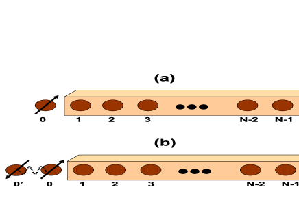
Figure 1: (Color online) Schematic picture for: (a) State transferring; (b) Entanglement distribution.

II set-up

The quantum channel consists of $N$ spin-1/2 particles sitting at sites $1$ to $N$ of a one dimensional lattice and interacting through the Hamiltonian

$$H_{\rm ch}=\sum_{l=1}^{N-1}\left(J_{x}\sigma^{x}_{l}\sigma^{x}_{l+1}+J_{y}\sigma^{y}_{l}\sigma^{y}_{l+1}+J_{z}\sigma^{z}_{l}\sigma^{z}_{l+1}\right)+h\sum_{l=1}^{N}\sigma_{l}^{z},$$ (1)

where $J_{\alpha}$ ($\alpha=x,y,z$) are the exchange integrals, $h$ is an external uniform magnetic field applied in the $z$ direction, and $\sigma_{l}^{\alpha}$ are the Pauli operators of the spin sitting at site $l$. We prepare the channel in some initial pure state $|\psi_{\rm ch}\rangle$, which can be either entangled or separable with respect to single-spin states. An extra qubit which carries the information is labelled by the site index $0$ and initially set in some arbitrary state $\rho_{{}_{0}}(0)$. The schematic picture of the system is shown in Fig. 1(a).

At $t=0$ the interaction between the qubit and the channel is suddenly switched on, via

$$H_{I}=J_{x}\sigma^{x}_{0}\sigma^{x}_{1}+J_{y}\sigma^{y}_{0}\sigma^{y}_{1}+J_{z}\sigma^{z}_{0}\sigma^{z}_{1}+h\,\sigma_{0}^{z}.$$ (2)

We use sudden switching for computational simplicity as the dynamics is not altered by a more realistic finite switching time, provided that it is small compared to the characteristic times set by the couplings of the Hamiltonian $H_{I}$ BBVB .

The total Hamiltonian $H=H_{\rm ch}+H_{I}$ rules the dynamics of the overall system, whose state at time $t$ reads

$$\rho(t)=e^{-iHt}\,\rho(0)\,e^{iHt}$$ (3)

where $\rho(0)=\rho_{{}_{0}}(0)\otimes|{\psi_{\rm ch}}\rangle\langle{\psi_{\rm ch}}|$ and $\hbar=1$. The density matrix of the qubit $N$, namely $\rho_{{}_{N}}(t)$, is obtained by tracing out the qubits $0,1,...,N-1$ from $\rho(t)$. On the other hand, one can define the superoperator $\mathcal{E}_{t}$ which maps the initial density matrix of the qubit 0, i.e. $\rho_{{}_{0}}(0)$, to the density matrix of qubit $N$ at time $t$, i.e. $\rho_{{}_{N}}(t)$, according to

$$\rho_{{}_{N}}(t)=\mathcal{E}_{t}[\rho_{{}_{0}}(0)].$$ (4)

When the transmission of a generic pure quantum state $|{\psi_{{}_{0}}}\rangle$ is in order, according to the scheme depicted in Fig. 1(a), we set $\rho_{{}_{0}}(0)\equiv|{\psi_{{}_{0}}}\rangle\langle{\psi_{{}_{0}}}|$ and quantify the quality of transmission by the fidelity $\langle\psi_{{}_{0}}|\rho_{{}_{N}}(t)|\psi_{{}_{0}}\rangle$ between the initial state $|\psi_{{}_{0}}\rangle$ and the final state $\rho_{{}_{N}}(t)$. In fact, the quality of the channel is better assessed by the average fidelity $\int d\psi_{{}_{0}}\langle\psi_{{}_{0}}|\rho_{{}_{N}}(t)|\psi_{{}_{0}}\rangle$, where integration is over the surface of the Bloch sphere and $d\psi_{{}_{0}}$ the corresponding measure. There are essentially two mechanisms that cause average fidelity to deteriorate during a transmission process of the type we are describing: dispersion, which is a collective phenomenon due to the channel being an interacting many-body system, and local rotations. As a matter of fact, the average fidelity does not distinguish between bad transmission, i.e. dispersion of the state all over the chain, and good transmission with an extra rotation during the dynamics; on the other hand, the latter can be safely handled with an extra unitary operation on the site $N$, thus leaving dispersion as the only destructive effect in transmitting quantum states.

Assume a unitary operator $R$, that does not depend on the state $|\psi_{{}_{0}}\rangle$, is found such that the average fidelity for the rotated final state $R^{\dagger}\rho_{{}_{N}}(t)R$ equals the maximum attainable value through the specific channel, then one could get a quantitative estimate of the dispersiveness of the transmission, which might be a very useful tool for characterizing the channel suitability for state transfer processes. Aiming at such goal, we introduce the Optimal Average Fidelity (OAF)

$$F(t)=\max_{R\in U(2)}\int d\psi_{{}_{0}}\langle{\psi_{{}_{0}}}|R^{\dagger}\mathcal{E}_{t}\left[|{\psi_{{}_{0}}}\rangle\langle{\psi_{{}_{0}}}|\right]R|{\psi_{{}_{0}}}\rangle~{},$$ (5)

where maximization over $R$ guarantees that the effect of local rotations is removed. It is of absolute relevance that, as shown in Appendix A, the OAF can be determined explicitly in terms of the superoperator $\mathcal{E}_{t}$

$$F(t)=\frac{1}{2}+\frac{1}{12}\left(m_{1}+m_{2}+\operatorname{sign}(\det(\mathcal{M}^{\mathcal{E}}))\,m_{3}\right)$$ (6)

where $m_{i}(t)$ are the singular values, in decreasing order, of the matrix

$$\mathcal{M}^{\mathcal{E}}_{mn}(t)=\operatorname{Tr}[\sigma_{m}\mathcal{E}_{t}(\sigma_{n})]~{},$$ (7)

where $\sigma_{n}$, $n=1,2,3$ are the Pauli matrices. The Optimal Average Fidelity, once computed via Eq. (6), gives a quantitative indication about how well a channel behaves, as far as the pure states transmission is concerned. Notice that the above expression has the very same form of the maximal fidelity with respect to maximally entangled states badziag , which, on the other hand is a completely different measure (an entanglement measure, in fact).

When entanglement distribution comes into play, mixed state transmission must be considered, and other strategies are necessary. Let us prepare qubit $0$ in a maximally entangled state with an isolated qubit $0^{\prime}$, see Fig. 1(b). The dynamical evolution cause the mixed state of qubit 0 to be transmitted to qubit $N$, thus generating entanglement between qubit $0^{\prime}$ and $N$. We can quantify the quality of such transmission by the amount of entanglement between qubits $0^{\prime}$ and $N$ at time $t$. For a generic spin chain, when qubits $0$ and $0^{\prime}$ are initially in the maximally entangled state $|\Phi^{+}\rangle=\left(|{00}\rangle+|{11}\rangle\right)/\sqrt{2}$ one can write

$$\rho_{{}_{0^{\prime}N}}(t)=(I\otimes\mathcal{E}_{t})\left[|\Phi^{+}\rangle\langle\Phi^{+}|\right],$$ (8)

where, $I$ represents the identity map. In the following, we use concurrence $C(\rho)$ as an entanglement measure concurrence for quantifying the amount of entanglement shared between qubits $0^{\prime}$ and $N$. Notice that different choices of initial maximally entangled state would give the same result, as the set of maximally entangled state can be obtained from $|{\Phi^{+}}\rangle$ through a local unitary operation in $0^{\prime}$, which is isolated.

Consistently with the transfer process, our scheme implies the existence of an arrival time when both the optimal average fidelity $F(t)$ and the concurrence $C(t)=C(\rho_{{}_{0^{\prime}N}}(t))$ get their maximum value. In fact, due to the finite size of the chain, the information travels from $0$ to $N$ and viceversa multiple times, and the above quantities displays multiple peaks during the dynamics. Throughout this paper we concentrate on the first peak, whose position defines the arrival time $t=t^{*}$, as in a practical situation waiting for longer times is unwise due to the effect of decoherence.

III FREE FERMIONIC SYSTEMS: XY HAMILTONIAN

In this section we consider the XY model defined by Eq. (1) with

$$J_{x}=J\frac{1+\gamma}{2},\ \ \ J_{y}=J\frac{1-\gamma}{2},\ \ \ J_{z}=0,$$ (9)

where, $J$ is the exchange coupling and $\gamma$ is the anisotropy parameter. This model is exactly solvable, as it turns into a free fermionic system, which makes valuable analytical results available. Despite being mapped into a non-interacting system, the model in the infinite $N$ limit has a rich phase diagram featuring a quantum phase transition sachdev at $h=1$ and, as far as the entanglement properties are concerned, the divergence of the entanglement range when approaching the curve $h^{2}+\gamma^{2}=1$, where pairwise entanglement vanishes paola1 ; paola2 ; paola3 . Moreover, its peculiar non equilibrium dynamics has been studied in the framework of dynamical entanglement sharing osterloh , with periodic boundary conditions assumed.

For diagonalizing this Hamiltonian one first maps spin operators $\sigma^{\pm}=(\sigma^{x}\pm i\sigma^{y})/2$ to fermionic operators through the Jordan-Wigner transformation $c_{l}=\prod_{n=0}^{l-1}\left(-\sigma_{n}^{z}\right)\sigma_{l}^{-}$ where $\{c_{l},c_{l^{\prime}}\}=0$ and $\{c_{l},c_{l^{\prime}}^{\dagger}\}=\delta_{l,l^{\prime}}$, as can be easily proven. The fermionic Hamiltonian can then be diagonalized with the procedure described in LiebSM1961 , of which we give a short summary in appendix B. The resulting diagonal Hamiltonian is

$$H=\sum_{k=0}^{N}E_{k}d_{k}^{\dagger}d_{k},$$ (10)

where the diagonal fermionic operators are obtained via the Bogolubov transformation

$$d_{k}=\sum_{l=0}^{N}P_{{}_{kl}}c_{l}+Q_{{}_{kl}}c_{l}^{\dagger}.$$ (11)

In the here considered case of finite $N$ and open boundary conditions the analytical expressions of the energies $E_{k}$ and of the matrices $P$, $Q$ for finite $\gamma$ and $h$ are complicated loginov , but they can be determined numerically as explained in appendix B.

The channel can be conveniently characterized in terms of its dynamical behaviour, which is investigated in the Heisenberg representation. The fermionic operators $c_{l}(t)=e^{+iHt}c_{l}e^{-iHt}$ read

$$c_{l}(t)=\sum_{n=0}^{N}U_{ln}(t)c_{n}+W_{ln}(t)c_{n}^{\dagger},$$ (12)

where,

$$U(t)= P^{T}e^{-itE}\,P+Q^{T}e^{+itE}\,Q,$$ (13)

$$W(t)= P^{T}e^{-itE}\,Q+Q^{T}e^{+itE}\,P,$$ (14)

$E$ is the diagonal energy matrix with elements $E_{k}$, and the inverse transformation Eq. (41) together with the identity $e^{+iHt}d_{k}e^{-iHt}=e^{-itE_{k}}d_{k}$ have been used. From the dynamical evolution of $c_{l}(t)$ that of the last-spin operators follow

$$\sigma_{N}^{-}(t)=\prod_{k=0}^{N}\left(-\sigma_{k}^{z}\right)\left[\sum_{l=0}^{N}U_{Nl}(t)c_{l}+W_{Nl}(t)c_{l}^{\dagger}\right],$$ (15)

where conservation of the parity $\prod_{l=0}^{N}(-\sigma_{l}^{z})$ is used.

We prepare the qubit $0$ in the density matrix which is parametrized by the vector $\vec{n}(0)$ of the Bloch sphere via $\rho_{0}(0)=(I+\vec{n}(0)\cdot\vec{\sigma})/2$. Correspondingly, the time evolution of the state of qubit $N$, $\rho_{N}(t)=(I+\vec{n}^{\prime}(t)\cdot\vec{\sigma})/2$, is parametrized by the vector $n^{\prime}_{\alpha}(t)=\langle{\Psi(0)}|\sigma^{\alpha}_{N}(t)|{\Psi(0)}\rangle$, which is determined from (15). Assuming that the channel is initialized in some state with constant parity $p$, i.e. $\prod_{k=1}^{N}\left(-\sigma_{k}^{z}\right)|\psi_{\rm ch}\rangle=(-1)^{p}|\psi_{\rm ch}\rangle$, our quantum channel (4) is described by the following affine transformation which maps vector $\vec{n}(0)$ of the Bloch sphere of qubit 0 to vector $\vec{n}^{\prime}(t)$ of the Bloch sphere of qubit $N$:

$$\begin{pmatrix}n^{\prime}_{x}\\ n^{\prime}_{y}\end{pmatrix} = S_{\phi_{w}-\phi_{u}}\begin{pmatrix}u-w&0\\ 0&u+w\end{pmatrix}S_{\phi_{w}+\phi_{u}}^{T}\begin{pmatrix}n_{x}\\ n_{y}\end{pmatrix}$$ (16)

$$n^{\prime}_{z}\phantom{\Big{)}} = n_{z}\big{(}u^{2}-w^{2}\big{)}+u^{2}+w^{2}+2A(t)-1$$ (18)

where $u(t)=|U_{N0}(t)|$, $w(t)=|W_{N0}(t)|$, $\phi_{u}(t)=\arg[U_{N0}(t)]+(p+1)\pi$, $\phi_{w}(t)=-\arg[W_{N0}(t)]+p\pi$, the rotation matrix is

$$S_{2\phi}=\begin{pmatrix}\sin\phi&\cos\phi\\ -\cos\phi&\sin\phi\end{pmatrix},$$ (19)

and $A(t)$ is the real function

$$A(t)=\sum_{j,l=1}^{N} U_{Nj}(t)^{*}U_{Nl}(t)\langle\psi_{\rm ch}|c_{j}^{\dagger}c_{l}|\psi_{\rm ch}\rangle+$$ (20)

$$W_{Nj}(t)^{*}W_{Nl}(t)\langle\psi_{\rm ch}|c_{j}c_{l}^{\dagger}|\psi_{\rm ch}\rangle+$$

$$U_{Nj}(t)^{*}W_{Nl}(t)\langle\psi_{\rm ch}|c_{j}^{\dagger}c_{l}^{\dagger}|\psi_{\rm ch}\rangle+$$

$$W_{Nj}(t)^{*}U_{Nl}(t)\langle\psi_{\rm ch}|c_{j}c_{l}|\psi_{\rm ch}\rangle.$$

Eqs. (16) show that the evolution in the $xy$-plane involves the two rotations $S_{\phi_{w}-\phi_{u}}$, $S_{\phi_{w}+\phi_{u}}^{T}$ as well as the shrinking towards the center of the Bloch sphere embodied in $u(t)-w(t)$ and $u(t)+w(t)$. Notice that none of the quantities involved depends on the initial state $|{\psi_{\rm ch}}\rangle$, thus relating the dynamics in the $xy$-plane only with the phase-diagram $\gamma$-$h$ of the model. In fact, the only dependence on the initial state is in the quantity $A(t)$ which uniquely affects the shift in the $z$ direction, and represents the interference of $|{\psi_{0}}\rangle$ with $|{\psi_{\rm ch}}\rangle$ during the evolution. Notice that in the XX case, where $W_{ij}(t)=0$ (see appendix C), the dynamics (16) realizes a generalized amplitude damping channel NielsenC2000 .

The OAF and the Concurrence can be calculated once the superoperator $\mathcal{E}_{t}$ is known. The elements of the superoperator $\mathcal{E}_{t}$ can be read from

$$\langle i|\rho_{{}_{N}}(t)|j\rangle=\sum_{k,l=0,1}\langle i|\mathcal{E}_{t}(|k\rangle\langle l|)|j\rangle\langle k|\rho_{{}_{0}}(0)|l\rangle.$$ (21)

From the elements $\langle i|\mathcal{E}(|k\rangle\langle l|)|j\rangle$ we can construct the Choi matrix $\mathcal{C}_{\mathcal{E}}(t)$

$$\langle{ki}|\mathcal{C}_{\mathcal{E}}(t)|{lj}\rangle=\langle i|\mathcal{E}_{t}(|k\rangle\langle l|)|j\rangle$$ (22)

which completely characterizes choi both the superoperator $\mathcal{E}_{t}$ and the state (8). By explicit calculation we have

$$\mathcal{C}_{\mathcal{E}}(t)=\left(\begin{array}[]{cccc}u(t)^{2}+A(t)&0&0&u(t)e^{i\phi_{u}(t)}\\ 0&1-u(t)^{2}-A(t)&w(t)e^{i\phi_{w}(t)}&0\\ 0&w(t)e^{-i\phi_{w}(t)}&w(t)^{2}+A(t)&0\\ u(t)e^{-i\phi_{u}(t)}&0&0&1-w(t)^{2}-A(t)\end{array}\right).$$ (23)

From the Choi matrix, using the procedure described in appendix A, we can compute the OAF: the singular values of $\mathcal{M}_{\mathcal{E}}$(t) are $2|u(t)+w(t)|$, $2|u(t)-w(t)|$, and $2|u(t)^{2}-w(t)^{2}|$, from which

$$F^{\rm XY}(t)=\frac{1}{2}+\frac{1}{6}\left|u(t)^{2}-w(t)^{2}\right|+\frac{1}{3}\max\{u(t),w(t)\}.$$ (24)

This is a remarkable result as it is fully independent of the initial state of the channel (i.e. the parameter $A(t)$) and depends only on the Hamiltonian parameters. Moreover, the rotation that maximizes the average fidelity is found to be

$$R=\begin{cases}e^{-i\frac{\phi_{u}}{2}\sigma^{z}}&\text{ for }u>w\\ e^{i\frac{\pi}{2}\sigma^{x}}e^{i\frac{\phi_{w}}{2}\sigma^{z}}&\text{ for }u<w\end{cases}.$$ (25)

In the XX case the effect of the magnetic field on the dynamics is only in the phase $\phi_{u}$, as shown in appendix C, and therefore one can always choose the magnetic field such that at the arrival time $t^{*}$, i.e. when fidelity peaks, $\phi_{u}(t^{*})=0$. On the other hand, in the XY case the dynamical quantities depends on $h$ in a complicated way, making the explicit rotation $R$, given in Eq. (25), necessary.

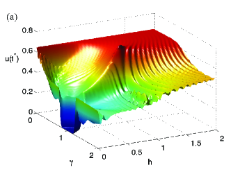
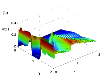
Figure 2: (Color online) (a) $u(t^{*})$ vs. $\gamma$ and $h$; the peak is located at $\gamma=0.7$ and $h=1$. (b) $w(t^{*})$ vs. $\gamma$ and $h$. Both figures are for $N=50$.

From Eq. (24) we see that the larger the difference between $u(t^{*})$ and $w(t^{*})$ the larger the OAF. In particular, as seen in Fig. 2, we find that, whenever the fidelity is large, we see $u(t^{*})\gg w(t^{*})$, so the qualitative behavior of the OAF is the same of $u(t^{*})$. Moreover, in the region $0\leq\gamma\leq 1$ and $1\leq h\leq 2$, $u(t^{*})$ is large, taking its maximum value for $\gamma=0$ (XX case) and for $\gamma=0.7$ and $h=1$. This means that in the $\gamma$-$h$ phase-diagram the line $\gamma=0$ and the point $(0.7,1)$ set the best possible Hamiltonian parameters, corresponding to the least dispersive channel.

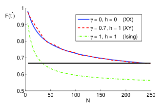
Figure 3: (Color online) Scaling of the OAF at the arrival time $t^{*}$ versus length $N$, for different parameters of the Hamiltonian.

The scaling of $F^{\rm XY}(t^{*})$ for increasing length $N$ is shown in Fig. 3 where it is clear that for the best parameters ($\gamma=0$, $h=0$ and $\gamma=0.7$, $h=1$) the OAF decreases very slowly, and it is greater than the classical value ($2/3$) even for chains up to $N=240$. This can be proved in the XX case thanks to the analytical results of appendix C. In fact, using Eq. (45), we can show that the solution of equation $F^{\rm XY}(t^{*})=2/3$ is $N=240$, in excellent agreement with Fig. 3. The weak dependence of $F^{\rm XY}(t^{*})$ on $N$ for the best parameters strengthens the statement that these indeed define the least dispersive channel, no matter the length. Conversely, for non optimal parameters (for example $\gamma=1$, $h=1$) the OAF decreases quickly and becomes lower than the classical threshold value $2/3$ for chains longer than $N=32$.

Let us now consider the entanglement distribution. We prepare the qubit pair $0^{\prime}$-$0$ in a pure entangled state, and let qubit 0 to be connected with the chain, while keeping $0^{\prime}$ isolated, so as to generate an entangled pair $0^{\prime}$-$N$. We use the concurrence concurrence to quantify the amount of entanglement in $\rho_{{}_{0^{\prime}N}}(t)$.

The density matrix of the qubit pair $0^{\prime}$-$N$, Eq. (8), is given by the Choi matrix as $\rho_{{}_{0^{\prime}N}}=\frac{1}{2}\mathcal{C}_{\mathcal{E}}$. The concurrence of this state is

$$C(t)=\max\{0,\;\hat{C}(u(t),w(t)),\;\hat{C}(w(t),u(t))\}$$ (26)

where,

$$\hat{C}(x,y)=x-\sqrt{(y^{2}+A(t))(1-x^{2}-A(t))}.$$ (27)

One can see that, at variance with the OAF, entanglement distribution depends on the initial state as it is a function of $A(t)$; this is due to the fact that during the dynamics the initial state of qubits 0 and $0^{\prime}$ interferes with the initial state of the chain and deteriorates the quality of the transmission.

In the following, we investigate different initial states of the channel in order to find out to which state a better quality transmission might correspond. In particular, we will refer to two fully separable states, namely the ferromagnetic state, with all the spins aligned along the $z$ direction, e.g. $|0,0,...,0\rangle$, and the Nèel state, with neighbouring spins antiparallel to each other, e.g. $|0,1,0,1,...,0,1\rangle$. Moreover, we will also study two different entangled initial states, namely that defined by a series of singlet states, and the ground state of the channel Hamiltonian.

Let us first consider the XX ($\gamma=0$) model, so as to exploit the analytical expressions available (see appendix C). We can prove that the concurrence achieves its maximum value, i.e. $u(t)$, when $|\psi_{\rm ch}\rangle$ is initialized in a ferromagnetic state. In fact in this case, since $W_{ij}(t)\equiv 0$, it is

$$A(t)=\sum_{j,l=1}^{N}U_{Nj}(t)^{*}U_{Nl}(t)\langle\psi_{\rm ch}|c_{j}^{\dagger}c_{l}|\psi_{\rm ch}\rangle.$$ (28)

which is equal to 0 (1) when $|\psi_{\rm ch}\rangle$ consists in a tensor product of down (up) spins. For other initial states, in which $0<A(t)<1$, the concurrence is lower than $u(t)$.

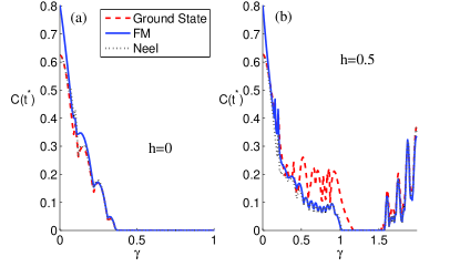
Figure 4: (Color online) Entanglement versus $\gamma$ in a chain of length $N=20$ for different initial states while the magnetic field takes: (a) $h=0$ and (b) $h=0.5J$.

In Fig. 4(a) we plot the concurrence as a function of anisotropy $\gamma$ when $h=0$ for different initial states. As the figure clearly shows increasing the anisotropy decreases the quality of transmission.

In the limit of $\gamma\rightarrow 1$ the Hamiltonian $H_{\rm ch}$ becomes Ising-like which has a poor transmitting quality. As one can see, in Fig. 4(a), in the absence of magnetic field the ferromagnetic initial state always gives the highest entanglement; in particular, when anisotropy $\gamma$ is small the difference between this initialization and the others is evident.

One may improve the poor ability of entanglement distribution in highly anisotropic chains (large $\gamma$) by switching on the magnetic field. This is clearly seen in Fig. 4(b) where we set $h=0.5$. Furthermore, we notice that the field does not essentially affect the transmission for small $\gamma$ and, quite surprisingly, makes the ground state the best possible initial state for strongly anisotropic chains.

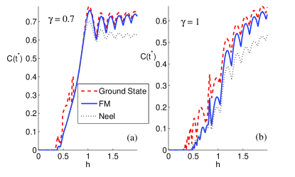
Figure 5: (Color online) Entanglement versus $h$ in a chain of length $N=20$ for different initial states while the anisotropy parameter takes: (a) $\gamma=0.7$ and (b) $\gamma=1$.

In order to better understand the role of magnetic field we consider the transmitted entanglement for different initial states as a function of $h$. In Fig. 5 we plot the concurrence for $\gamma=0.7$ and $\gamma=1$ and see that there exists a value of the field, slightly depending on the initial state of the chain, above which the transmission becomes possible, even for large anisotropies.

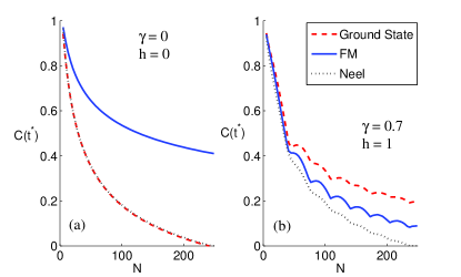
Figure 6: (Color online) Scaling of the obtained entanglement at the arrival time versus length $N$ for different initial states: (a) isotropic XX Hamiltonian ($\gamma=0$ and $h=0$); (b) anisotropic XY Hamiltonian ($\gamma=0.7$ and $h=1$).

The existence of an exact solution for the XY Hamiltonian allows us to study the quality of transmission for very long chains. In Fig. 6 we plot $C(t^{*})$ as a function of $N$ for different initial states, which evidently differentiate the entanglement transmission through long chains. In particular, in Fig. 6(a), we see that in the XX chain the ferromagnetic initial state not only gives the highest concurrence amongst the different initializations but it also provides the best scaling with $N$. In Fig. 6(b) we plot $C(t^{*})$ as a function of $N$ for $\gamma=0.7$ and $h=1$, i.e. for the parameteres that defines the less dispersive XY-like channel (see Fig. 2). At variance with the state transmission case, where for such parameters the transmission quality is as high as in the XX case (see Fig. 3), during entanglement distribution through an XY chain we can not avoid the interference $A(t)$ by properly choosing the initial state of the chain, and a strong dependence on the length $N$ appears; Fig. 6(b) in fact shows that this gives rise to a significant lowering of the transferred concurrence.

Results for the Nèel state and the series of singlets are found to be very close to each other (therefore only those for the former state are plotted): This shows that the inherent entanglement in the initial state has a very little effect when a state is attached at one end of a spin chain.

IV Interacting Systems: XXZ Hamiltonian

After studying the effect of the initial state on the transmission quality of the channel in free fermionic systems, interacting models must also be considered, not only because they represent the large majority of many-body systems, but also because they are usually characterized by an extremely rich, though often difficult to be physically deciphered, phenomenology.

Amongst the interacting Hamiltonians the XXZ spin model here discussed, and defined by Eq. (1) with

$$J_{x}=J_{y}=\frac{J}{2},\hskip 28.45274ptJ_{z}=\frac{J\Delta}{2}~{},$$ (29)

is known to describe many real systems and compounds, thus playing an essential role, especially in one dimensional physics mikeska ; Lukin2003 .

This model has a very rich phase diagram: $\Delta<-1$ is the ferromagnetic phase with a simple separable ground state with all spins aligned to the same direction. For $-1<\Delta\leq 1$ the Hamiltonian is gapless and the region is called $XY$ phase. $\Delta>1$ defines the Nèel phase, where the spectrum is gapped and a finite staggered magnetization arises. In the Ising limit $\Delta\gg 1$ the ground state is the Nèel state.

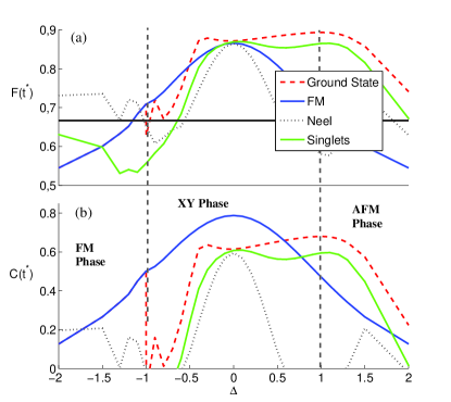
Figure 7: (Color online) Transferring properties of a XXZ chain with the length of $N=20$ in its whole phase diagram for different initial states: (a) optimized average fidelity at the arrival time $t^{*}$ (the black line indicates the classically obtained fidelity $2/3$); (b) obtainable entanglement at the arrival time $t^{*}$.

Dynamical transmission in interacting fermionic models is very different from the free fermionic case, as it results from a complex combination of many different effects amongst which the scattering between interacting excitations and the existence of localized states. As a matter of fact, there is no transmission process which is generally independent on the initial state of the channel. In particular we find that, depending on the value of $\Delta$, the best transmission processes correspond to different initializations of the chain.

Let us first discuss the state transfer process. In Fig. 7(a) we see that even the OAF strongly depends on $|{\psi_{\rm ch}}\rangle$: for $\Delta>0$ the ground state clearly gives the best possible initialization, while for $\Delta<0$ the phenomenology is much more complicated. When considering the entanglement distribution in Fig. 7(b) the situation is somehow reversed, with a specific state, namely the ferromagnetic one, granting the best possible initialization for $\Delta<0$, and a more complex scenario for $\Delta>0$.

The general phase diagram in Fig. 7 embodies the complex balance between the effect of interference, which can be varied by acting on the initial state of the chain, and the dispersiveness of the channel which depends on $\Delta$. As we already noted, in the XXZ case also the OAF is affected by interference, and the overlap of $F(t^{*})$ observed in Fig. 7(a) in the $\Delta=0$ point is due to its corresponding to a non-interacting model, for which, as proved in section III, the OAF does not depend on the initial state. On the other hand, there is no $\Delta$ value where the entanglement distribution is independent on the destructive effects of interference. Therefore, the only mechanism for removing such effect is that of choosing a ferromagnetic initial state, whose dynamics can be resolved in the single particle sector bose where interference does not occur. The absence of interference is the reason why for $\Delta=0$ the $C(t^{*})$ obtained with the ferromagnetic initial state is by far larger then the others. Finally, in Figs. 7(a) and (b) we see that, given the initial state, $F(t^{*})-2/3$ and $C(t^{*})$ have a similar behaviour as a function of $\Delta$, with a shift in $C(t^{*})$ for the FM initial state, consistent with the exact analysis given above for the XX case.

Indications about the effects of dispersiveness of the channel on the transmission processes can also be extracted: the ground state is seen to minimize such effects for whatever $\Delta$, though this implies a better entanglement distribution only for $\Delta>0.5$ where interference probably plays a minor role leaving dispersion as the main destructive effect.

V Conclusion

In this paper we have studied the quality of state and entanglement transmission through quantum channels described by spin chains varying both the Hamiltonian parameters and the initial state of the channel. We have considered a vast class of Hamiltonians, including interacting and non-interacting fermionic systems, which contains some of the most relevant experimental realizations of one dimensional many-body systems, both in the framework of solid state physics and in the realm of cold atoms in optical lattices.

We find that if a free-fermionic model is available and an XY-like spin Hamiltonian can be effectively realized, then the best possible tuning of the parameters is that corresponding to the XX model with a ferromagnetic initial state, both for state and entanglement transfer, whose quality stays surprisingly high even for chains as long as $N\simeq 240$. In the anisotropic case, a state transfer of the same quality as that attained at $\gamma=0$, is obtained for $\gamma=0.7$ and $h=1$: referring to the framework developed in Ref. BACVV2010 , we infer that the relevant excitations lie in the linear zone of the dispersion relation and the resulting dynamics is essentially dispersionless. Moreover, good results for both state and entanglement transmission are found in a wide range of the parameters $\gamma$ and $h$, providing the channel is initialized in its ground state. When an interacting XXZ model with a specific $\Delta$ is at hand, one has to choose whether to optimize the state or the entanglement transmission, since these goals are obtained with different initial states. In fact, we find that the optimal average fidelity is more sensitive to the dispersiveness of the channel, while the entanglement distribution is more sensitive to the interference with the initial state of the chain. As a matter of fact the former gets its maximum in the antiferromagnetic isotropic ($\Delta=1$) channel initialized in its ground state, while the latter is maximized by an XX ($\Delta=0$) channel initialized in a ferromagnetic state.

Our analysis show that the fidelity and the entanglement do not necessarily quantify the quality of quantum communication in the same way. Namely, highest entanglement transfer can occur along a spin chain which is different from that giving the highest average fidelity. In fact, to the best of our knowledge, these results are the first example in which state and entanglement transmission show different features due to the different role played in such processes by dispersion, essentially set by the parameters of the Hamiltonian, and interference, which explicitly depends on the initial state of the channel. However, when we have higher entanglement one can always purify/distill entanglement using local operations bennett-distillation and subsequently use it for teleportation and eventually end up with a higher fidelity.

Acknowledgement:- LB and PV gratefully acknowledge usefull discussions with T. J. G. Apollaro, A. Cuccoli, and R. Vaia. AB and SB acknowledge the EPSRC. SB also thanks the Royal Society and the Wolfson Foundation.

Appendix A Optimal average fidelity

In this section we derive an explicit expression for calculating the optimal average fidelity (OAV) defined in Eq. (5). Using the results of Ref. horofidel

$$\frac{3}{2} \max_{R\in U(2)}\int d\psi_{{}_{0}}\langle{\psi_{{}_{0}}}|R^{\dagger}\mathcal{E}\left[|{\psi_{{}_{0}}}\rangle\langle{\psi_{{}_{0}}}|\right]R|{\psi_{{}_{0}}}\rangle-\frac{1}{2}=$$

$$\max_{R\in U(2)}\langle{\Phi^{+}}|(I\otimes R^{\dagger}\,\mathcal{E})\left[|{\Phi^{+}}\rangle\langle{\Phi^{+}}|\right](I\otimes R)|{\Phi^{+}}\rangle=$$

$$\max_{|{\psi_{\rm me}}\rangle}\;\langle{\psi_{\rm me}}|(I\otimes\mathcal{E})\left[|{\Phi^{+}}\rangle\langle{\Phi^{+}}|\right]|{\psi_{\rm me}}\rangle,$$ (30)

since $(I\otimes R)|{\Phi^{+}}\rangle$, for varying unitary matrix $R$, generates every maximally entangled state $|{\psi_{\rm me}}\rangle$. Moreover, in badziag it was proved that

$$\max_{|{\psi_{\rm me}}\rangle}\langle{\psi_{\rm me}}|\rho|{\psi_{\rm me}}\rangle=\frac{1}{4}\left(1+t_{1}+t_{2}-\operatorname{sign}(\det(T))t_{3}\right)$$ (31)

where $T_{mn}=\operatorname{Tr}[\rho\,\sigma_{m}\otimes\sigma_{n}]$ and $t_{i}$ are the singular values of $T$, i.e. the square root of the eigenvalues of $T^{T}T$, in decreasing order. The explicit expression of equations (6) and (7) follows directly from Eqs. (A),(31) and for the properties of Choi matrix $\mathcal{C}_{\mathcal{E}}\equiv(I\otimes\mathcal{E})\left[2|{\Phi^{+}}\rangle\langle{\Phi^{+}}|\right]$ which can be easily proved from its definition (22). In fact,

$$\mathcal{M}^{\mathcal{E}}_{mn} =\operatorname{Tr}[\sigma_{m}\mathcal{E}(\sigma_{n})]=\operatorname{Tr}\left[\mathcal{C^{\mathcal{E}}}\sigma_{n}^{T}\otimes\sigma_{m}\right]=$$

$$=(-1)^{n+1}\operatorname{Tr}\left[\mathcal{C^{\mathcal{E}}}\sigma_{n}\otimes\sigma_{m}\right].$$ (32)

Appendix B Diagonalization of the XY chain

The total XY Hamiltonian is

$$H_{\gamma}=J\sum_{k=0}^{N-1}\{\sigma_{k}^{+}\sigma_{k+1}^{-}+\gamma\sigma_{k}^{+}\sigma_{k+1}^{+}+\text{h.c.}\}+h\sum_{k=0}^{N}\sigma_{k}^{z}.$$ (33)

which, by substituting the spin operators with their fermionic counterparts takes the form

$$H=\sum_{k,l=0}^{N}\{c_{k}^{\dagger}A_{kl}c_{l}+\frac{1}{2}(c_{k}^{\dagger}B_{kl}c_{l}^{\dagger}-c_{k}B_{kl}c_{l})\},$$ (34)

where, $A$ is a symmetric matrix with elements $A_{kl}=J(\delta_{k,l+1}+\delta_{k,l-1})+h\delta_{k,l}$ and $B$ is an anti-symmetric matrix with elements $B_{kl}=\gamma(\delta_{k,l-1}-\delta_{k,l+1})$. The above quadratic Hamiltonian can be diagonalized in the form (10) using a Bogoliubov transformation (11), and the diagonalization process reduces to finding the energies $E_{k}$ and the matrices $P$ and $Q$. From Eq. (10)

$$[H,d_{k}]=E_{k}d_{k}^{\dagger}.$$ (35)

and then, by using Eq. (34) and (11) the conditions read

$$AP^{T}+BQ^{T} = +P^{T}E$$ (36)

$$AQ^{T}+BP^{T} = -Q^{T}E$$ (37)

where, $E$ is a diagonal matrix with elements $E_{kl}=E_{k}\delta_{k,l}$. To ensure that the transformation (11) be canonical and invertible the matrices have to satisfy these conditions

$$PP^{T}+QQ^{T} = P^{T}P+Q^{T}Q=\bar{I}_{N+1}$$ (38)

$$PQ^{T}+QP^{T} = P^{T}Q+Q^{T}P=0,$$ (39)

which can be simplified by defining the new matrices $\alpha=P+Q$ and $\beta=P-Q$. In fact, Eqs. (38) force $\alpha$ and $\beta$ to be orthogonal matrices. Moreover, since $(A+B)^{T}=A-B$, Eqs. (36) simplifies into a single equation

$$A-B=\alpha^{T}E\beta$$ (40)

which is the singular value decomposition of the matrix $A-B$. The desired matrices $P=(\alpha+\beta)/2$ and $Q=(\alpha-\beta)/2$ are computed accordingly and the diagonalization process is completed.

For completeness we show also the inverse transformation that easily comes from (38)

$$c_{k} = \sum_{l=0}^{N}P_{{}_{lk}}d_{l}+Q_{{}_{lk}}d_{l}^{\dagger},$$ (41)

$$c_{k}^{\dagger} = \sum_{l=0}^{N}P_{{}_{lk}}d_{l}^{\dagger}+Q_{{}_{lk}}d_{l}.$$ (42)

Appendix C Analytical evaluation of $u(t)$ in the XX model

In the XX model we have $E_{k}=2J\cos(\frac{\pi(k+1)}{N+2})+2h$, $P_{kn}=\sqrt{\frac{2}{N+2}}\sin(\frac{\pi(k+1)(n+1)}{N+2})$ and $Q_{kn}=0$, making $W_{kn}(t)\equiv 0$. Since the magnetic field causes only a constant shift in the dispersion relation, in the following we set $h=0$. In this case

$$U_{{}_{N0}}(t) =\sum_{k=0}^{N}e^{-itE_{k}}P_{k0}P_{kN}$$

$$=\sum_{m=1}^{\infty}i^{-m}\mathcal{J}_{m}(\beta)\sum_{k=0}^{N}\cos\left(\frac{\pi m(k+1)}{N+2}\right)P_{k0}P_{kN}$$

$$\simeq i^{-N}\big{(}\mathcal{J}_{N}(\beta)+2\mathcal{J}_{N+2}(\beta)+\mathcal{J}_{N+4}(\beta)\big{)}$$

$$=\frac{4}{i^{N}}\left[\left(\frac{N+2}{\beta}\right)^{2}\mathcal{J}_{N+2}(\beta)-\frac{\mathcal{J}_{N+2}^{\prime}(\beta)}{\beta}\right]$$ (43)

where $\beta=2Jt$. In the above equation we used the Jacobi-Anger expansion and some properties of the Bessel function $\mathcal{J}_{n}$ abramowitz . The approximation consists in neglecting the Bessel functions of order $m(N+2)$, with $m\geq 2$, since they contribute only after times of order $\frac{mN}{2J}$. In fact, one can show that at the transmission time $t^{*}$, i.e. the time when $U_{{}_{N0}}(t)$ takes its first peak, $\beta^{*}\equiv 2Jt^{*}\simeq N-\xi(N/2)^{\frac{1}{3}}$. Using the properties of Bessel function abramowitz

$$u(t^{*})=\frac{2^{\frac{7}{3}}}{N^{\frac{1}{3}}}\operatorname{Ai}(\xi)+\frac{2\xi}{5N}\left(3\xi\operatorname{Ai}^{\prime}(\xi)+22\operatorname{Ai}(\xi)\right)$$ (44)

where $\operatorname{Ai}(\xi)$ is the Airy function. It can be proved bose that the maximum of $u(t^{*})$ is reached for $\xi=-1.019$ and thus

$$u(t^{*})=\frac{2.700}{N^{\frac{1}{3}}}-\frac{4.804}{N}.$$ (45)

References

- (1) G. M. Nikolopoulos, D. Petrosyan and P. Lambropoulos, J. Phys.: Condens. Matter 16, 4991 (2004); G. M. Nikolopoulos, D. Petrosyan and P. Lambropoulos, Europhys. Lett. 65, 297 (2004).
- (2) J. M. Taylor, et al., Nature Phys. 1, 177 (2005).
- (3) S. Bose, Contemporary Physics 48, 13 (2007).
- (4) S. Bose, Phys. Rev. Lett. 91, 207901 (2003).
- (5) A. Bayat, S. Bose, Phys. Rev. A 81, 012304 (2010).
- (6) M. Steiner, J. Villain, C.G. Windsor, Advances in Physics 25, 87 (1976).
- (7) H-J. Mikeska and A. Kolezhuk, Lect. Notes Phys. 645, 1, (2004).
- (8) W. S. Bakr et al., Nature 462, 74 (2009).
- (9) G. K. Brennen et al., Phys. Rev. Lett. 82, 1060 (1999).
- (10) O. Mandel et al., Nature 425, 937 (2003).
- (11) M. Greiner et al., Nature 415, 39 (2002).
- (12) J. F. Sherson, et al., Nature 467, 68 (2010); W. S. Bakr, et al., Science 329, 547 (2010); M. Karski et al., New J. Phys. 12, 065027 (2010).
- (13) L. Duan, E. Demler and M. D. Lukin, Phys. Rev. Lett. 91, 090402 (2003).
- (14) C. Weitenberg, et al., arXiv:1101.2076.
- (15) A. Koetsier, R. A. Duine, I. Bloch, H. T. C. Stoof, Phys. Rev. A 77, 023623 (2008).
- (16) P. Barmettler, et al., Phys. Rev. A 78, 012330 (2008).
- (17) P. Medley, et al., Phys. Rev. Lett. 106, 195301 (2011).
- (18) M. Christandl et al., Phys. Rev. Lett. 92, 187902 (2004).
- (19) C. Di Franco, M. Paternostro, D. I. Tsomokos, S. F. Huelga, Phys. Rev. A 77, 062337 (2008).
- (20) C. Di Franco, M. Paternostro, M. S. Kim, Phys. Rev. Lett. 101, 230502 (2007).
- (21) N. Y. Yao et al., Phys. Rev. Lett. 106, 040505 (2011); N. Y. Yao et al., arXiv:1012.2864.
- (22) L. Banchi, T. J. G. Apollaro, A. Cuccoli, R. Vaia, P. Verrucchi, Phys. Rev. A 82 052321 , (2010); L. Banchi, T. J. G. Apollaro, A. Cuccoli, R. Vaia, P. Verrucchi, arXiv:1105.6058.
- (23) L. Banchi, A. Bayat, P. Verrucchi, S. Bose, Phys. Rev. Lett. 106, 140501 (2011).
- (24) P. Badzia¸g, M. Horodecki, P. Horodecki, and R. Horodecki, Phys. Rev. A 62, 012311 (2000).
- (25) W. K. Wootters, Phys. Rev. Lett., 80, 2245 (1998).
- (26) S. Sachdev, Quantum phase transitions, Cambridge University Press, 1999.
- (27) T. Roscilde, P. Verrucchi, A. Fubini, S. Haas, V. Tognetti, Phys. Rev. Lett. 93, 167203, (2004).
- (28) L. Amico, F. Baroni, A. Fubini, D. Patane, V. Tognetti, P. Verrucchi, Phys. Rev. A 74, 022322, (2006).
- (29) F. Baroni, A. Fuini, V. Tognetti, P. Verrucchi, J. Phys. A 32, 9845 (2007).
- (30) L. Amico, A. Osterloh, F. Plastina, R. Fazio, G. M. Palma, Phys. Rev. A 69 022304, (2004)
- (31) E. Lieb, T. Schultz and D. Mattis, Ann. Phys. 16, 407 (1961).
- (32) A. V. Loginov, Y. V. Pereverzev, Low Temp. Phys. 23, 534 (1997).
- (33) M. A. Nielsen and I. L. Chuang, Quantum information and computation (Cambridge University Press, Cambridge, 2000).
- (34) M. Choi, Linear Algebra and its Applications 10, 285 (1975).
- (35) C. H. Bennett, et al., Phys. Rev. Lett. 76, 722 (1996).
- (36) M. Horodecki, P. Horodecki, and R. Horodecki, Phys. Rev. A 60, 1888 (1999).
- (37) M. Abramowitz and I. A. Stegun, Handbook of Mathematical Functions (Dover, New York, 1972).