A phenomenology analysis of the tachyon warm inflation in loop quantum cosmology

Abstract

We investigate the warm inflation condition in loop quantum cosmology. In our consideration, the system is described by a tachyon field interacted with radiation. The exponential potential function, $V(\phi)=V_{0}e^{-\alpha\phi}$, with the same order parameters $V_{0}$ and $\alpha$, is taken as an example of this tachyon warm inflation model. We find that, for the strong dissipative regime, the total number of e-folds is less than the one in the classical scenario, and for the weak dissipative regime, the beginning time of the warm inflation will be later than the tachyon (cool) inflation.

I Introduction

The inflation is a very important concept in the modern cosmology Liddle-book . The standard model of the inflation was introduced by Guth Guth-in . However, because this model relies on a scalar field which has no interaction with any other fields, so that it is impossible that the radiation to be produced during the inflation. This leads to a thermodynamically supercooled phase of the Universe Berera-Warm . So this standard inflationary model needs a ”graceful exit” to ensure the Universe enters a radiation-dominated phase. In fact, it is not the only way to describe the inflationary dynamics. Another model of the inflationary picture is called the warm inflation Berera-Warm , as opposed to the conventional cool inflation. In this model, the dissipative effects are very important during the inflationary era, so the radiation is produced concurrently with an inflationary expansion and there is no a separate reheating phase. Also, the density fluctuation in the warm inflation arises from the thermal fluctuation, rather than the vacuum fluctuation which dominates the supercooled case Berera-Fang . The radiation dominates immediately as soon as the warm inflation ends. The matter components of the Universe are created by the decay of either the remaining inflationary field or the dominant radiation field Berera-1996PRD .

The warm inflation has been studied by many authors not only in classical cosmology scenario but also in quantum cosmology scenario (see Berera-Warm and references therein, and Herrera-tach ; Herrera-quan ). In this paper, we focus on a tachyon warm inflation in loop quantum cosmology (LQC) scenario.

The application of loop quantum gravity techniques to homogeneous cosmological models is known as LQC Bojowald-1-11 ; Ashtekar-1-12 ; Singh-1-13 . Owing to the homogeneity and isotropy of the spacetimes, the connection is determined by a single parameter called $c$ and the triad is determined by $p$. The variables $c$ and $p$ are canonically conjugate with Poisson bracket $\{c,p\}=\gamma\kappa/3$, in which $\gamma$ is the Barbero-Immirzi parameter and $\kappa=8\pi G$. In the LQC scenario, the initial singularity is instead by a bounce. Thanks to the quantum effect, the Universe is in an initially contracting phase with minimal but not zero volume, and then the quantum effect drives it to the expanding phase. And, in the effective LQC scenario, the loop quantum effects can be very well described by a effective modified Friedmann dynamics Singh-PRD ; Taveras-PRD . There are two types of modifications, one is the inverse volume correction, the other is the holonomy correction. This paper we just discuss the holonomy correction. In this effective LQC scenario, a factor of $(1-\rho/\rho_{c})$ is added to the standard Friedmann equation. For the correction term, $-\rho/\rho_{c}$, comes with a negative sign, the Hubble parameter $H$, and $\dot{a}$ vanishes when $\rho=\rho_{c}$, consequently the quantum bounce occurs.

The warm inflation in the LQC scenario is considered by Herrera Herrera-LQC recently. The author discussed the inflationary phenomenon described by a scalar field coupled to radiation. In this paper, we would like to consider a tachyon warm inflation in the LQC scenario. The tachyon field might be responsible for the inflation at the early stage and could contribute to some new form of dark matter at late times Sen-JHEP . The behavior of the tachyon field in LQC was studied by Sen-PRD , in which the author considered the inverse volume modification and found that there exists a super accelerated phase in the semiclassical region. (For arbitrary matter, the Universe will enter a super accelerated phase, this issue was first considered by Singh-CQG .) The tachyon field in LQC based on $\rho^{2}$ modification was studied by Xiong-tach . The authors found that the inflation could be extended to the region where the classical inflation stops. In this paper, we consider the tachyon field is interacting with radiation during the inflationary stage. Just as many authors have pointed out (see Samart-dy ,ect) the dynamical behaviors of interacting field in LQC are very different from the ones in classical cosmology. The purpose of this paper is comparing the difference between the tachyon warm inflation in LQC and the one in classical cosmology, and also, we will compare the difference between the tachyon warm inflation and the tachyon (cool) inflation in LQC.

The paper is organized as follows. We present in Sec. II the basic concepts of the tachyon warm inflation in the LQC scenario, and discuss in Sec. III the exponential potential as an example of this tachyon warm inflation. We end this paper with some conclusions and discussions in Sec. IV .

II Tachyon warm inflation in LQC

In the LQC scenario, the Friedmann equation is modified as Ashtekar-1-16 ; Ashtekar-1-17

$$H^{2}=\frac{\kappa}{3}\rho\left(1-\frac{\rho}{\rho_{c}}\right),$$ (1)

with the total energy density $\rho$ and the critical density $\rho_{c}$, and $\kappa=8\pi G$. In our consideration, $\rho=\rho_{\phi}+\rho_{\gamma}$, where $\rho_{\phi}$ denotes the energy density of the tachyon field $\phi$, and $\rho_{\gamma}$ the radiation energy density.

The dynamical equations for $\rho_{\phi},\rho_{\gamma}$ in the warm inflation scenario are

$$\dot{\rho}_{\phi} = -3H(\rho_{\phi}+p_{\phi})-\Gamma\dot{\phi}^{2},$$ (2)

$$\dot{\rho}_{\gamma} = -4H\rho_{\gamma}+\Gamma\dot{\phi}^{2},$$ (3)

where the dot means the derivation with respect to time, and $\Gamma$ is the dissipation coefficient responsible for the decay of energy density of the tachyon field into radiation during the inflationary era. $\Gamma$ can be considered as a constant or a function of the field $\phi$, or the temperature $T$, or both of them Herrera-tach ; and, according to the second law of thermodynamics, $\Gamma>0$ should be hold. In this paper, for simplicity we only consider to be a constant. The energy density $\rho_{\phi}$ and the pressure $p_{\phi}$ of the tachyon field can be written as Sen-PRD

$$\rho_{\phi}=\frac{V(\phi)}{\sqrt{1-\dot{\phi}^{2}}},\qquad p_{\phi}=-V(\phi)\sqrt{1-\dot{\phi}^{2}},$$ (4)

in which $V(\phi)$ is the potential of the tachyon field.

Considering Eqs.(2) and (4), one can get the equation of motion (EoM) of the tachyon field

$$\frac{\ddot{\phi}}{1-\dot{\phi}^{2}}+3H\dot{\phi}+\frac{V_{,\phi}}{V(\phi)}=-\frac{\Gamma\dot{\phi}}{V(\phi)}\sqrt{1-\dot{\phi}^{2}},$$ (5)

in which $V_{,\phi}=\frac{dV(\phi)}{d\phi}$.

In the LQC scenario, the condition for a bounce is $H=0$ and $\dot{H}>0$, in which

$$\dot{H}=-\frac{\kappa}{6}\left[3\rho(\phi)\dot{\phi}^{2}+4\rho_{\gamma}\right]\left(1-2\frac{\rho_{\phi}+\rho_{\gamma}}{\rho_{c}}\right).$$ (6)

This means that the Universe will enter a super-inflation phase immediately after bouncing. This is the first stage of the inflation. The Hubble parameter $H$ will be increasing in this stage. This stage is purely cased by the quantum effect and is very short Chiou-inf . We don’t consider it in this paper.

According to Eqs.(1) and (6), the Raychaudhuri equation can be written as

$$\frac{\ddot{a}}{a} = \dot{H}+H^{2}=H^{2}\left(1-\varepsilon\right)$$

$$= -\frac{\kappa}{6}\left\{\rho\left(1-\frac{\rho}{\rho_{c}}\right)+3\left[p\left(1-\frac{2\rho}{\rho_{c}}\right)-\frac{\rho^{2}}{\rho_{c}}\right]\right\},$$

with the total pressure $p=p_{\phi}+p_{\gamma}$ and the slow-roll parameter $\varepsilon=-\frac{\dot{H}}{H^{2}}$. Inflation is often defined as a period of accelerated expansion, i.e., $\ddot{a}>0$. In this paper, we will focus on the evolution of the field in the slow-roll inflationary era. During this era, the potential dominates over the kinetic energy of the tachyon field, i.e. $\rho_{\phi}\simeq V(\phi)$, and the energy density of the radiation, i.e., $V(\phi)>\rho_{\gamma}$. We can also assume that $\dot{\phi}^{2}\ll 1$ and $\ddot{\phi}\ll[3H+\Gamma/V(\phi)]\dot{\phi}$ in this region. Then, the Friedmann equation is reduced to

$$H^{2}=\frac{\kappa}{3}V(\phi)\left(1-\frac{V(\phi)}{\rho_{c}}\right).$$ (7)

And the EoM of the tachyon field (5) becomes

$$3H(1+R)\dot{\phi}=-\frac{V_{,\phi}}{V(\phi)},$$ (8)

in which $R$ is the rate defined as

$$R=\frac{\Gamma}{3HV(\phi)}.$$ (9)

For a strong (weak) dissipative regime, we have $R\gg 1$ ($R<1$), i.e., $\Gamma\gg 3HV$ ($\Gamma<3HV$).

The Raychaudhuri equation can be rewritten as

$$\frac{\ddot{a}}{a}=-\frac{\kappa}{6}\left(\rho_{\rm{eff}}+3p_{\rm{eff}}\right),$$ (10)

with

$$\rho_{\rm{eff}}=\rho_{\phi}\left(1-\frac{\rho_{\phi}}{\rho_{c}}\right),\quad p_{\rm{eff}}=p_{\phi}\left(1-\frac{2\rho_{\phi}}{\rho_{c}}\right)-\frac{\rho_{\phi}^{2}}{\rho_{c}}.$$ (11)

The inflation ends when $\ddot{a}=0$, this implies that $\rho_{\rm{eff}}+3p_{\rm{eff}}=0$. So, at the point of ending of the inflation, one has

$$\rho_{\phi}=\frac{3\omega+1}{3\omega+4}\rho_{c},$$ (12)

with the equation of state parameter of the tachyon field $\omega=p_{\phi}/\rho_{\phi}$. In the classical cosmology, $\rho\ll\rho_{c}$, it is easy to find that the inflation ends when $\rho_{\phi}=-3p_{\phi}$, i.e., $\omega=-\frac{1}{3}$ (see Eq.(10) and consider $\frac{\rho_{\phi}}{\rho_{c}}=0$). But in the LQC scenario, if $\omega=-\frac{1}{3}$, $\rho_{\phi}=0$, this means the energy density of the tachyon field should be zero at the inflation ending point. But it is easy to verify that $\rho_{\phi}>0$ when $\omega=-\frac{1}{3}$ (see Eq.(4)). This means that the inflation phase still exists in LQC while the classical inflation stops. Notice that we suppose the quantum effect can not be ignored. If $\rho_{\phi}\ll\rho_{c}$ where the quantum effect can ge ignored, just as Xiong-tach argued, the quantum and the classical inflation have the same trajectory. This phenomena is as same as the tachyon (cool) inflation in LQC. This is not surprise. For the energy density of the tachyon field (or the potential of the tachyon field) dominates over the energy density of radiation.

Also, as the condition is in the classical tachyon warm inflation Herrera-tach , we can consider that the radiation production is qusi-stable during the warm inflation region. Then the energy density of radiation can be reduced as

$$\rho_{\gamma}=\frac{\Gamma\dot{\phi}^{2}}{4H}.$$ (13)

Considering Eqs.(7), (8) and (13), one can obtain

$$\rho_{\gamma}=\frac{R}{4\kappa(1+R)^{2}}\frac{V_{,\phi}^{2}}{V(\phi)^{2}(1-V(\phi)/\rho_{c})}.$$ (14)

Under those conditions, one can get the slow-roll parameter

$$\varepsilon=\frac{1}{2\kappa}\frac{1}{V(\phi)(1+R)}\left(\frac{V_{,\phi}}{V(\phi)}\right)^{2}\frac{[1-2V(\phi)/\rho_{c}]}{[1-V(\phi)/\rho_{c}]^{2}}.$$ (15)

The last fraction is caused by the modification of the quantum geometry. Also, we can rewrite $\varepsilon$ as a function of $\rho_{\gamma},\rho_{\phi}$ and the rate $R$:

$$\varepsilon=\frac{\rho_{\gamma}}{\rho_{\phi}}\frac{2(1+R)}{R}\frac{1-2\rho_{\phi}/\rho_{c}}{1-\rho_{\phi}/\rho_{c}}.$$ (16)

The accelerated expansion occurs if $\varepsilon<1$, i.e., $\ddot{a}>0$. Then, the relationship between $\rho_{\phi}$ and $\rho_{\gamma}$ in the accelerated region is

$$\frac{2(1+R)}{R}\rho_{\gamma}<\frac{1-\rho_{\phi}/\rho_{c}}{1-2\rho_{\phi}/\rho_{c}}\rho_{\phi}.$$ (17)

The inflation ends when the slow-roll conditions are violated, i.e., $\varepsilon=1$, which implies

$$\left(\frac{V_{,\phi}}{V(\phi)}\right)^{2}\frac{[1-2V(\phi)/\rho_{c}]}{\kappa V(\phi)[1-V(\phi)/\rho_{c}]^{2}}=2(1+R).$$ (18)

The number of e-folds before inflation ends is

$$N(\phi)=\kappa\int^{\phi_{i}}_{\phi_{f}}\frac{V(\phi)^{2}[1-V(\phi)/\rho_{c}]}{V_{,\phi}}(1+R)d\phi.$$ (19)

in which $\phi_{i},\phi_{f}$ denote the values of the tachyon field at the beginning and the end of inflation respectively.

Comparing above equations with the ones in the classical scenario Herrera-tach , one can find that the term modified by quantum geometry is very important in the inflationary regions. Notice that we assume the inflation happens very near the quantum dominated region. If the inflation happens far away from the quantum dominated region, then the quantal modified term $\frac{\rho}{\rho_{c}}=0$ and the variables which are shown by above equation are as same as the ones in the classical cosmology. As an example, we will discuss the warm inflation of the tachyon field with an exponential potential in strong and weak dissipative regime.

III An example: exponential potential

At the Sec. II we get the expressions for the variables of the tachyon warm inflation with general potential. As an example, we consider in this section the exponential potential Sen-MPLA

$$V(\phi)=V_{0}e^{-\alpha\phi},$$ (20)

with the constant $V_{0}>0$ and the tachyon mass $\alpha>0$ (with unit $m_{p}$). The discussion will be concerned with the strong and weak dissipative regime. For simplicity, we just consider $\Gamma=\Gamma_{0}$ is a constant.

III.1 Warm inflation in the strong dissipative regime

For a strong dissipative regime, we have $R\gg 1$, i.e., $\Gamma\gg 3HV$. Considering Eqs.(8) and (20), one can get

$$\Gamma\dot{\phi}=V_{0}\alpha e^{-\alpha\phi}.$$ (21)

Here, we have taken into account the condition of $\Gamma\gg 3HV$. And from now on, we will just consider $\Gamma$ as a constant dissipation coefficient, i.e., $\Gamma=\Gamma_{0}$. Then, one can obtain the evolution of the tachyonic field:

$$\phi(t)=\frac{1}{\alpha}\ln\left(\frac{\alpha^{2}V_{0}}{\Gamma_{0}}t+e^{\alpha\phi_{i}}\right),$$ (22)

in which $\phi_{i}$ is the initial value of $\phi$ at the time that the slow-roll inflation begins. It is straightforward to see that $\phi(t)$ is not the function of the quantum geometry correction $\left(1-V(\phi)/\rho_{c}\right)$. This is because we consider $\Gamma\gg 3HV$, then the Hubble parameter is ignored when we consider the EoM of the field. This is as same as the evolution in the tachyon warm inflation of the classical cosmology scenario Herrera-tach , but is different from the standard inflation of tachyon field in LQC Xiong-tach in which the correction came from the quantum geometry effects plays an important role.

To get an explicit expression of the number of e-folds, we will resort to the values of the potential at the beginning and the end of the inflation. According to Eq.(19), we can get

$$N_{Strong}(V)=\frac{\Gamma_{0}}{\alpha^{2}}\sqrt{\frac{3}{\kappa}}\int^{V_{i}}_{V_{f}}\frac{\sqrt{1-V/\rho_{c}}}{V^{3/2}}dV,$$ (23)

in which $V_{i},V_{f}$ denote the values of the potential of the tachyon field at the beginning and the end of the the inflation respectively. The inflation ends when $\ddot{a}=0$, i.e., $H^{2}_{f}=-\dot{H}_{f}$. This implies that

$$\frac{\kappa}{3}V_{f}\left(1-\frac{V_{f}}{\rho_{c}}\right)=\frac{\kappa}{2}V_{f}\dot{\phi}^{2}_{f}\left(1-\frac{2V_{f}}{\rho_{c}}\right)=\frac{\kappa^{2}}{2\Gamma^{2}_{0}}V^{3}_{f}\left(1-\frac{2V_{f}}{\rho_{c}}\right).$$

We have used Eqs.(6), (7), (8) and (9), and the slow-roll approximate $\rho_{\phi}\simeq V(\phi),\rho_{\phi}\gg\rho_{\gamma}$. Solving the above equation, one can get

$$V_{f}=V(\phi=\phi_{f}) = \frac{1}{6}{\frac{\sqrt[3]{-30\rho_{{c}}\alpha{\Gamma_{0}}^{2}+{\rho_{{c}}}^{3}{\alpha}^{3}+2\Gamma_{0}\sqrt{-16{\Gamma_{0}}^{4}+213{\Gamma_{0}}^{2}{\rho_{{c}}}^{2}{\alpha}^{2}-18\,{\rho_{{c}}}^{4}{\alpha}^{4}}}}{\alpha}}$$ (24)

$$+\frac{1}{6}{\frac{4{\Gamma_{0}}^{2}+{\rho_{{c}}}^{2}{\alpha}^{2}}{\alpha\sqrt[3]{-30\,\rho_{{c}}\alpha\,{\Gamma_{0}}^{2}+{\rho_{{c}}}^{3}{\alpha}^{3}+2\Gamma_{0}\sqrt{-16{\Gamma_{0}}^{4}+213\,{\Gamma_{0}}^{2}{\rho_{{c}}}^{2}{\alpha}^{2}-18{\rho_{{c}}}^{4}{\alpha}^{4}}}}}+\frac{1}{6}\rho_{{c}}.$$

Obviously, this result depends on the values of $\Gamma_{0},\alpha$ and $\rho_{c}$.

Integrating Eq.(23), one can get

$$N_{Strong}(V)=\left.\frac{\Gamma_{0}}{\alpha^{2}}\sqrt{\frac{3}{\kappa}}\left[2\,{\frac{\rho_{{c}}-V}{\sqrt{V\left(\rho_{{c}}-V\right)\rho_{{c}}}}}+\arctan\left({\frac{\sqrt{\rho_{{c}}}\left(-1/2\,\rho_{{c}}+V\right)}{\sqrt{-\rho_{{c}}{V}^{2}+{\rho_{{c}}}^{2}V}}}\right){\frac{1}{\sqrt{\rho_{{c}}}}}\right]\right|_{V_{i}}^{V_{f}}.$$ (25)

The number of e-folds depends on $V_{i}=V_{0}\exp^{-\alpha\phi_{i}}$ and $V_{f}$ given in Eq.(24). To ensure $V_{f}$ is a real number, $-16{\Gamma_{0}}^{4}+213{\Gamma_{0}}^{2}{\rho_{{c}}}^{2}{\alpha}^{2}-18{\rho_{{c}}}^{4}{\alpha}^{4}>0$ should be held. This gives a constraint on $\Gamma_{0},\alpha$, i.e., $0.32<\frac{\Gamma_{0}}{\alpha}<2.25$. This means the same order of the magnitude of $\Gamma_{0},\alpha$. Note that this order of the magnitude of $\alpha$ is smaller than the one who used in the tachyon (cool) inflation Xiong-tach . Always, the observational data gives a constraint on the value of $\Gamma_{0}$, just as the jobs of Herrera-tach . This constraint connects with the spectrum of the scalar perturbations and the tensor-scalar ratio. But unfortunately, the holonomy correction to the scalar perturbation is still incomplete, even for the scalar field. So, the value of $\Gamma_{0},\alpha$ is still need for more research.

If the quantum correction can be ignored, the total e-folding number will less than 1 when one discusses the strong dissipation in the classical cosmology Herrera-tach . To compare the total e-folding number in LQC and the one in classical cosmology, we can employ the slow roll condition and approximately replace the term $\left(1-V\left(\phi\right)/\rho_{c}\right)$ by a constant $\lambda<1$ Xiong-tach . Under this approximation, the Hubble parameter can be rewritten as

$$\frac{\dot{a}}{a}\simeq\sqrt{\frac{\kappa}{3}\lambda V(\phi)}.$$ (26)

Considering Eqs.(20) and (22), one can get

$$\frac{a}{a_{i}}=\exp\left[\frac{2\Gamma_{0}}{V_{0}\alpha}\sqrt{\frac{\kappa\lambda V_{0}}{3}}\left(\sqrt{\frac{\alpha^{2}V_{0}}{\Gamma_{0}}t+e^{\alpha\phi_{i}}}-e^{\frac{1}{2}\alpha\phi_{i}}\right)\right],$$ (27)

with the initial value $a_{i}$ of $a$ at the time at the beginning of the inflation $t_{i}$. For $0<\lambda<1$, the scale factor in this region is smaller than the one in classical scenario Herrera-tach . Based on Eq.(27), one can get the time at the end of the inflation $t_{f}$, i.e., the time of $\ddot{a}=0$.

$$t_{f}=\frac{3\alpha^{2}}{4\kappa\lambda\Gamma_{0}}-\frac{\Gamma_{0}}{\alpha^{2}V_{0}}e^{\alpha\phi_{i}}.$$ (28)

And, this time is bigger than the one in classical scenario Herrera-tach . Inserting this equation into Eq.(27), one can obtain Sami-info

$$\frac{a_{f}}{a_{i}}=\exp\left[\frac{2\Gamma_{0}}{V_{0}\alpha}\left(\sqrt{\frac{\alpha^{4}V^{2}_{0}}{4\Gamma_{0}^{2}}-\frac{\kappa\lambda V_{0}}{3}e^{\alpha\phi_{i}}}-e^{\frac{1}{2}\alpha\phi_{i}}\right)\right].$$ (29)

It is easy to find that, for an exponential potential in slow-roll limit, the number of e-folds of the tachyon warm inflation in LQC is smaller than the classical one. This is caused by the quantum correction. Then it is not surprise that this result is as same as the ones in tachyon (cool) inflation Xiong-tach . So, if we believe the quantum effect cannot be ignored, then the e-folding number will small than the one in classical cosmology. This means that $N_{Strong}<1$ for the strong dissipative regime. The tachyon field will become bigger and bigger during the slow-roll inflation, then $V=V_{0}e^{-\alpha\phi}$ will become smaller and smaller, so $\lambda=(1-V/\rho_{c})$ will become smaller and smaller during the slow-roll inflation scenario. This means that $\frac{a_{f}}{a_{i}}$ will be bigger than the one which is described by Eq.(29). But the total number of e-folds in LQC is smaller than the one in classical cosmology. Notice that the total number of e-folds in LQC did not include the e-folds of super-inflation.

III.2 Warm inflation in the weak dissipative regime

The tachyon warm inflation in the weak dissipative regime in classical cosmology was discussed by Herrera-weak . Considering $\Gamma=const.$ and the weak dissipation, i.e., $R<1$, the total number of e-folds can be rewritten as

$$N_{Weak}(\phi) = \kappa\int^{\phi_{i}}_{\phi_{f}}\frac{V(\phi)^{2}[1-V(\phi)/\rho_{c}]}{V_{,\phi}}d\phi$$ (30)

It is obvious that $N_{Weak}(\phi)$ depends on the tachyon mass $\alpha$ and the relationship between $V$ (this means that it also dependents on $V_{0}$) and $\rho_{c}$. In Herrera-weak , the authors shown $V_{0}\sim 10^{-10}m_{p}^{4}$ and $\alpha\sim 10^{-6}m_{p}$. These data are based on the WMAP five-year data and the Sloan Digital Sky Survey (SDSS) large-scale structure surveys and the perturbations of the tachyon field in the classical cosmology scenario. If these data is still tenable in the LQC scenario, then $V(\phi)\ll\rho_{c}$ for $\phi\gg-2.3\times 10^{7}$ ($V(\phi)\simeq\rho_{c}$ for $\phi=-2.3\times 10^{7}$). Then the quantum effect can be ignored. The total number of e-folds of the tachyon warm inflation in the weak dissipative regime in LQC scenario is as same as the one in the classical scenario. But as same as we mentioned before, the perturbation theory of the tachyon field in the LQC scenario is still need for more study, then we cannot obtain $V_{0},\alpha$ through the observe data. The main aim of this subsection is comparing the difference between the tachyon warm inflation and the tachyon (cool) inflation in LQC, we assume $V_{0}=0.82,\alpha=0.5$. And these differences are shown in the Fig.1.

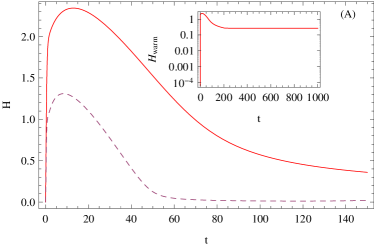
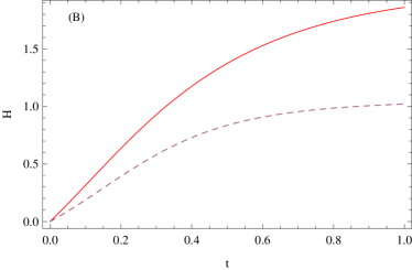
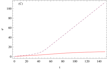
Figure 1: (Color online). Evolutions for the case of the tachyon warm inflation (solid curve) and the tachyon (cool) inflation (dashed curve) with $V_{0}=0.82,\alpha=0.5,\Gamma=0.1$ and $\rho_{\gamma}(t=0)=0$. (A). Evolution of the Hubble rate $H$. The first period after bouncing is super-inflation ($H$ is increasing. This period is shown in the (B)), and then $H$ decrease till the inflation stage. The sub-picture in (A) is the evolution of $H$ in warm inflation. (C). Evolution of the tachyon field $\phi$ with exponential potential $V=V_{0}e^{-\alpha\phi}.$ Unlike the scalar field with the quadratic potential that it will enter an oscillatory epoch, the tachyon field will always increase.

Figure 1 shows that there are two stages of the inflation. The first is a stage of the super-inflation near the bouncing epoch as we discussed in the Sec.II. It is easy to find that the super-inflation ends very quickly. The second stage of the inflation begins at the stage $H\simeq Const.$. This stage is far away from the bouncing epoch and the quantum correction is completely negligible. This is nothing but just the standard slow-roll inflation.

The evolution pictures of two inflationary scenario have the same directions when we consider the same initial condition ($\phi(t=0)=0,\dot{\phi}(t=0)=0,a(t=0)=1,\dot{a}(t=0)=0$). The variable $H$ in warm inflation is bigger than the one in (cool) inflation at the same time. This is reasonable. Since the total energy density $\rho$ in warm inflation includes the energy density of the tachyon field $\rho_{\phi}$ and the radiation $\rho_{\gamma}$, but the one in (cool) inflation just includes $\rho_{\phi}$. We assume these two different inflation models have the same initial conditions. So $\rho>\rho_{\phi}$ at the same time. And we can find that the field $\phi$ in warm inflation is smaller than the one in (cool) inflation. This is because the energy density of the tachyon field decays into the radiation during the inflationary era. Also, we can see the non-inflationary phase (between the super-inflation and the slow-roll inflation) in warm inflation is longer than the one in (cool) inflation. This phase is an indirect loop quantum gravity effect Chiou-inf . It is easy to find that the slow-roll inflation is beginning at $t\simeq 48$ in the (cool) inflation but at $t\simeq 200$ in the warm inflation.

In this section, we discuss the warm inflation of the tachyon field with an exponential potential in the LQC scenario. We find that the total number of e-fold is less than 1 if we consider the strong dissipative regime ($R\gg 1$). And if we consider the weak dissipative regime ($R<1$), the beginning time of the slow-roll inflation in warm inflation is later than the one in (cool) inflation when we consider the same initial condition. But due to the perturbation theory of loop quantum cosmology is still open, we cannot get the parameters $V_{0},\alpha$ through the observational data. Therefore it is still impossible to get the special total number of e-folds number.

IV conclusions and discussions

As showing in Eq.(1), the Friedmann equation in LQC adds a factor of $(1-\rho/\rho_{c})$ in the right side of the standard Friedmann equation. The correction term $\rho/\rho_{c}$ comes with a negative sign, this makes it possible that $\dot{a}=0$ when $\rho=\rho_{c}$, and the bounce occurs. At the bounce point, $H=0$ and $\dot{H}$ is positive. The Universe enters a super-inflation stage. (If one considers the inverse volume modification, the Universe will also enter a super-inflation stage Singh-CQG .) Eq.(6) shows that $\dot{H}$ continues to positive till $\rho=\frac{1}{2}\rho_{c}$ (at which point $\dot{H}$ is vanishes, and after this point, it will become negative.). Thus, every LQC solution has a super-inflation phase from $\rho=\rho_{c}$ to $\rho=\frac{1}{2}\rho_{c}$. However, we must recognize that this stage is very short, so that the super-inflation can not substitute for the slow-roll inflation.

In this paper, we studied the tachyon warm inflation model in the LQC scenario. At first, we considered the tachyon field with a general potential coupled with radiation field in the slow-roll inflation phase. During this inflationary era, the potential dominates over the kinetic energy of the tachyon field and the energy density of radiation. Then the modified Friedmann equation and Rachaudhuri equation have the same expressions with the tachyon (cool) inflation in LQC. We found that the warm inflation phase in LQC will expand to the region where the classical inflation stops. The interacting term will modify the EoM of the tachyon field in the slow-roll approximate. Then the energy density of radiation has also been modified. Based on those conditions, we got a general relationship between the tachyon field and radiation energy density, and obtained the relationship between $\rho_{\gamma},\rho_{\phi}$ in the accelerated region. We found that the number of e-folds before inflation ends depends on the modification term $(1-V(\phi)/\rho_{c})$ and the rate $R$.

And then, as an example, we discussed the tachyon warm inflation with an exponential potential in a strong and a weak dissipative regime. For the strong dissipative regime ($\Gamma\gg 3HV$), the quantum geometry effects did not change the evolution of the tachyon field $\phi(t)$. But it will modify the energy density of radiation, the scale factor, and the total number of e-folds. We found that the total number of e-folds in LQC is less than the one in the classical scenario if we just consider the slow-roll inflation phase. We also discussed the difference between the tachyon warm inflation in the weak dissipative regime and the tachyon (cool) inflation in LQC. We found that the Hubble parameter $H$ in warm inflation is bigger than the one in (cool) inflation at the same time, the beginning time of slow-roll inflation in warm inflation is later then the one in (cool) inflation, and the value of the tachyon field $\phi$ at the beginning time of warm inflation is less than the one in (cool) inflation.